Distributed coordinated path following using guiding vector fields
←
→
Page content transcription
If your browser does not render page correctly, please read the page content below

Distributed coordinated path following using guiding vector
fields
Citation for published version (APA):
Yao, W., Garcia de Marina, H., Sun, Z., & Cao, M. (2021). Distributed coordinated path following using guiding
vector fields. arXiv, 2021, [2103.12372]. http://adsabs.harvard.edu/abs/2021arXiv210312372Y

Document status and date:
Published: 01/03/2021

Please check the document version of this publication:
• A submitted manuscript is the version of the article upon submission and before peer-review. There can be
important differences between the submitted version and the official published version of record. People
interested in the research are advised to contact the author for the final version of the publication, or visit the
DOI to the publisher's website.
• The final author version and the galley proof are versions of the publication after peer review.
• The final published version features the final layout of the paper including the volume, issue and page
numbers.
Link to publication

General rights
Copyright and moral rights for the publications made accessible in the public portal are retained by the authors and/or other copyright owners
and it is a condition of accessing publications that users recognise and abide by the legal requirements associated with these rights.

       • Users may download and print one copy of any publication from the public portal for the purpose of private study or research.
       • You may not further distribute the material or use it for any profit-making activity or commercial gain
       • You may freely distribute the URL identifying the publication in the public portal.

If the publication is distributed under the terms of Article 25fa of the Dutch Copyright Act, indicated by the “Taverne” license above, please
follow below link for the End User Agreement:
www.tue.nl/taverne

Take down policy
If you believe that this document breaches copyright please contact us at:
openaccess@tue.nl
providing details and we will investigate your claim.

Download date: 14. Nov. 2021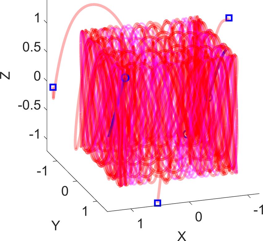
Distributed coordinated path following using guiding vector fields
Weijia Yao, Hector Garcia de Marina, Zhiyong Sun, Ming Cao
Abstract— It is essential in many applications to impose a aircraft flying at a constant speed such that the aircraft
scalable coordinated motion control on a large group of mobile asymptotically follow a circular path of the same radius
robots, which is efficient in tasks requiring repetitive execution, while keeping user-specified distances. Another work [6]
such as environmental monitoring. In this paper, we design a
guiding vector field to guide multiple robots to follow possibly designs different potential functions to derive a guiding
different desired paths while coordinating their motions. The vector field for multiple robots, but their motions cannot be
vector field uses a path parameter as a virtual coordinate explicitly coordinated (e.g., the multi-robot distance cannot be
arXiv:2103.12372v2 [cs.RO] 9 Apr 2021
that is communicated among neighboring robots. Then, the controlled). These two studies only consider some common
virtual coordinate is utilized to control the relative parametric desired paths, such as a circle or a straight line in 2D. The
displacement between robots along the paths. This enables us
to design a saturated control algorithm for a Dubins-car-like paper [7] provides a decentralized control law such that
model. The algorithm is distributed, scalable, and applicable multiple robots can circulate a closed curve in 3D, but the
for any smooth paths in an n-dimensional configuration space, curve must have a specific form, and some strong assumptions
and global convergence is guaranteed. Simulations with up to on the integral curves are required.
fifty robots and outdoor experiments with fixed-wing aircraft There are many studies on coordinated path-following
validate the theoretical results.
without employing a guiding vector field. The robots’ motions
I. I NTRODUCTION in [8] are coordinated by using a virtual structure when
following predefined paths. However, each robot needs to
One of the grand challenges in robotics is the reliable
broadcast its states and reference trajectories to the rest of
and systematic coordination of a large number of robots
the robots, so the communication burden increases rapidly as
without a central nexus [1]. Tasks involving vast geographic
the size of the multi-robot systems increases. Recently, [9]
areas or volumes, such as search and rescue, patrolling,
proposes a distributed hybrid control law based on [10] to
and environmental monitoring, are practically impossible
coordinate the robot motions such that robots keep a constant
for a single robot, while multiple coordinated robots can
parametric separation. A similar task is achieved by another
deal with such scenarios efficiently. In these applications, it
recent work in [11]. However, these two studies, as well as
is fundamental for a group of robots to accurately follow
many others (e.g., [12]–[14]), are restricted to planar or simple
possibly different paths, while coordinating their motions to
desired paths, such as a straight line. Another related work
form a formation which satisfies some geometric or parametric
[15] only considers planar simple closed curves and unit-speed
constraints. In this paper, we design a coordinating vector field
particles, and the convergence result is valid locally. In [16],
to guide multiple robots to converge to their respective desired
an output-regulation controller is applied to certain robots
paths and realize the aforementioned coordinated behavior in
while other robots are controlled through local interactions.
a distributed way through local information exchange.
This approach is effective, but the desired motion must be
Related work: Many path-following algorithms for a
periodic and generated by a linear exosystem.
single robot have been studied in the literature, such as
Multi-robot coordinated path following control has been
Line-of-sight (LOS) [2] among others [3]. Among several
extensively studied in the specialized cases of circular
tested algorithms, those using a guiding vector field are
formation control and circumnavigation control. In circular
shown to achieve the highest path-following accuracy while
formation control, multiple robots either need to move to
requiring the least control efforts [3]. However, to the best
or initially start on a specified circle, and then move along
of our knowledge, there are only a few studies on extending
the circle until some desired arc distances are achieved via
the guiding vector field approach to realize multi-robot
local communication [17]–[23]. Circumnavigation control
coordinated path following tasks. Utilizing the guiding vector
additionally requires all robots to keep moving along the
field in [4], the work [5] employs a distributed algorithm to
circle to fulfill some tasks, such as escorting an important
change the radii of the circular paths for each fixed-wing
target [24]–[32]. However, these studies are all restricted
Weijia Yao and Ming Cao are with the University of Groningen, the to 2D circular paths, and many of them impose additional
Netherlands. {w.yao,m.cao}@rug.nl Hector Garcia de Marina is requirements on the robots’ initial positions (e.g., to maintain
with Universidad Complutense de Madrid, Spain. hgarciad@ucm.es the order preservation [21], [22]). The paper [33] presents a
Zhiyong Sun is with the Eindhoven University of Technology, the Netherlands.
z.sun@tue.nl The work of Cao was supported in part by the European decentralized controller for robots characterized by the double-
Research Council (ERC-CoG-771687) and the Netherlands Organization integrator model such that they can generate 2D desired
for Scientific Research (NWO-vidi-14134). The work of Yao is supported geometric patterns composed of simple closed curves. This
in part by the China Scholarship Council. The work of Hector Garcia de
Marina is supported by the grant Atraccion de Talento 2019-T2/TIC-13503 work is extended in [34] for robots described by the single-
from the Government of the Autonomous Community of Madrid. integrator model to circulate a closed curve. However, these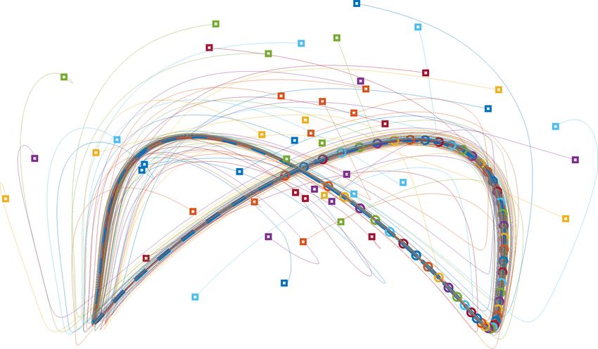
two studies are both restricted to 2D closed curves.                   functions; i.e., P hgh := {ξ ∈ Rn+1 : φi (ξ) = 0, i ∈ Zn1 }.
   Contributions: We propose a coordinating vector field to            The projection of P hgh on the plane spanned by the first
enable distributed coordinated path following for multiple             n coordinates is the original desired path P phy , so we can
robots, and a corresponding saturated control algorithm is             use the higher-dimensional guiding vector field χ : Rn+1 →
designed for a Dubins-car-like model. In particular, we use            Rn+1 corresponding to P hgh to make a robot follow the
the path parameter as an additional virtual coordinate for             original desired path P phy by projecting to the n-dimensional
the guiding vector field, and this virtual coordinate is further       space [36], where
communicated among neighboring robots to achieve motion                                                   Xn
coordination. There are many appealing features of our                        χ(ξ) = × ∇φi , . . . , ∇φn −            ki φi ∇φi , (1)
                                                                                                                  i=1
approach: 1) It is distributed and scalable, and thus applicable
for a team of an arbitrary number of robots; 2) It can deal            with ki > 0, ∇φi ∈ Rn+1 being the gradient of φi
with complex paths such as self-intersecting, non-convex, or           with respect to the generalized coordinate ξ, and ×(·)
non-closed ones in an n-dimensional configuration space. 3)            being the wedge product [42, Chapter 7.2]. The physical
Given a fixed communication frequency, the communication               interpretation
                                                                          Pn            of the vector field χ is clear: the second term
burden is low since every two neighboring robots only                  − i=1 ki φi ∇φi is a weighted sum of all the gradients,
need to transmit and receive at most two scalars (i.e., the            which guides the robot trajectory towards the intersection of
virtual coordinate and its time derivative); 4) It guarantees          the hyper-surfaces(i.e., the desired path), while the first term
that the coordinated path-following control objectives are             × ∇φi , . . . , ∇φn , being orthogonal to all the gradients [42,
achieved globally regardless of robots’ initial positions. 5) The      Proposition 7.2.1], provides a propagation direction along the
approach has been verified by simulations with a large multi-          desired path.
robot system and by experiments with fixed-wing aircraft in               In our previous work [36], [43], this higher-dimensional
a windy environment. We also show that our approach is                 guiding vector field in (1) is proved to possess no singular
promising in area or volume coverage tasks by exploiting a             points, where the vector field becomes zero, thanks to the
2D or 3D Lissajous curve with irrational coefficients, as it is        additional dimension (i.e., the additional virtual coordinate
guaranteed that robots can eventually visit every point of an          w). However, like many other current studies (e.g., [38], [39],
area or volume while keeping prescribed distances.                     [44]), the vector field is used for the guidance of only one
   Notations: The notation Zji represents the set {m ∈ Z :             single robot. We aim to extend the vector field to include
i ≤ m ≤ j}. We use boldface for a vector v ∈ Rn , and its              a coordination component and achieve motion coordination
i-th entry is denoted by vi for i ∈ Zn1 . Consider a system            among multiple robots. Since the additional virtual coordinate
consisting of N robots, and a vector ui ∈ Rn for i ∈ ZN         1 ,    w not only helps eliminate singular points, but also acts as
then for j ∈ Zn1 , the notation uij refers to the j-th entry of ui .   the path parameter, one idea is to utilize the virtual coordinate
Graphs: We call V := {1, . . . , N } the node set representing         w to coordinate the robots’ motions. Thus, the question is:
the robots, and E ⊆ (V × V) is the edge set encoding the                  Question: Suppose there are N robots. Based on the higher-
communication links. We call Ni := {j ∈ V : (i, j) ∈ E} the            dimensional vector field in (1), how can one design an extra
set of neighbors of robot i. In this paper, we only consider           coordination mechanism using the virtual coordinates wi ,
undirected graphs, which implies that if (i, j) ∈ E, then Robot        i ∈ ZN1 , such that 1) Each robot can follow their desired paths;
i and Robot j can share information bidirectionally. Please            2) All robots can coordinate their motions by controlling the
see [35] for an introduction to graph theory.                          virtual coordinates wi , i ∈ ZN1 via local information exchange
                                                                       among neighbors?
                      II. P RELIMINARIES
                                                                          The extra coordination mechanism and the precise mean-
   Guiding vector fields with virtual coordinates for robot            ing of motion coordination will become clear in the next
navigation enjoy many desirable features, such as guarantee-           section, where a mathematical problem formulation based on
ing global convergence to the desired path and enabling                dynamical systems theory will be presented.
self-intersecting desired path following [36]. We present
here a brief introduction. Suppose the desired path P phy                    III. D ESIGN OF GUIDING VECTOR FIELDS FOR
is parameterized by x1 = f1 (w), . . . , xn = fn (w), where xi                          MULTI - ROBOT SYSTEMS
is the i-th coordinate, w ∈ R is the parameter of the path
and fi is twice continuously differentiable (i.e., fi ∈ C 2 ),         A. Mathematical problem formulation
for i ∈ Zn1 . To derive a corresponding guiding vector field,             The i-th robot is required to follow a path in Rn , parame-
one needs to describe the desired path as the intersection             terized by n parametric equations:
of n hyper-surfaces [37]–[41]. To this end, taking w as an
additional argument, one defines n surface functions φi :                          xi1 = fi1 (wi )   ...   xin = fin (wi ),         (2)
Rn+1 → R as follows: φi (ξ) = xi −fi (w) for i ∈ Zn1 , where
ξ = (x1 , . . . , xn , w) ∈ Rn+1 is the generalized coordinate         where xij is the j-th coordinate, fij ∈ C 2 is the j-th
with an additional (virtual) coordinate w. Therefore, the              parametric function for the i-th robot, for i ∈ ZN           n
                                                                                                                          1 , j ∈ Z1 ,
desired path with an additional coordinate is the intersection         and wi ∈ R is the parameter of the desired path. To derive the
of the hyper-surfaces described by the zero-level set of these         path-following guiding vector field, we use the parameter wi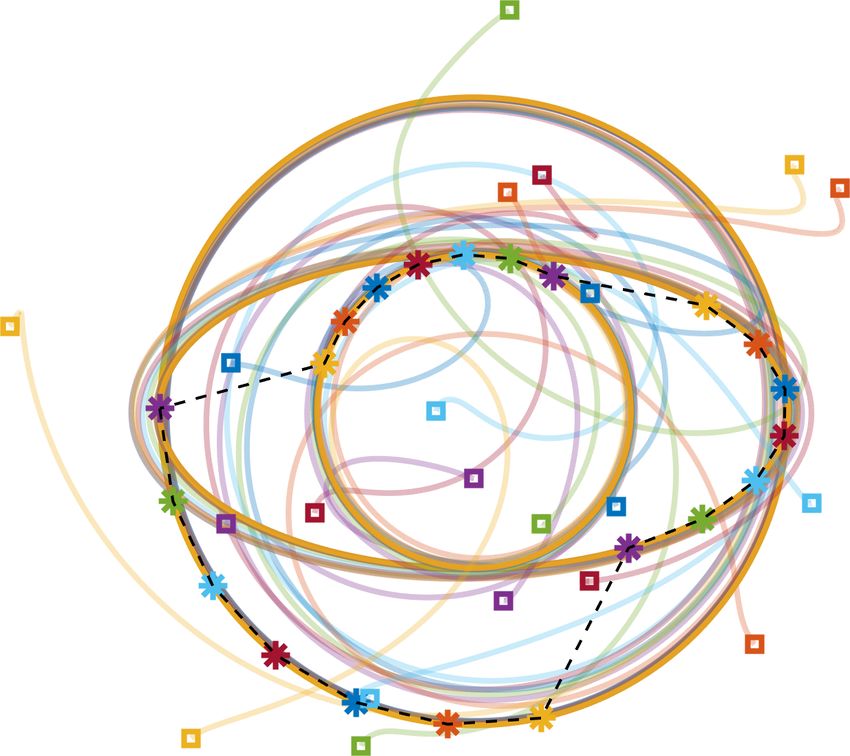
as an additional virtual coordinate, and the higher-dimensional Problem 1. Design the coordinating vector field Xi in (5)
desired path is described by for i ∈ ZN1 , such that the trajectories of (6), given an initial
condition ξ0 ∈ R(n+1)N , fulfill the two control objectives:
Pi := {ξi ∈ Rn+1 : φi1 (ξi ) = 0, . . . , φin (ξi ) = 0},
1) (Path Following) Robot i’s path following error to its
where ξi := (xi1 , . . . , xin , wi ) ∈ Rn+1 denotes the general- desired path Pi converges to zero asymptotically for all
ized coordinate of the i-th robot, and the surface functions i ∈ ZN1 . That is, kΦi (ξi (t)k → 0 as t → ∞, ∀i ∈ Z1 .
N
are φij = xij − fij (wi ) for i ∈ ZN n
1 and j ∈ Z1 . Define 2) (Motion Coordination) Each robot’s motion is coordi-
Φi (ξi ) := (φi1 (ξi ), . . . , φin (ξi ))> ∈ Rn . Observe that nated distributedly subject to the communication graph
ξi ∈ Pi if and only if kΦi (ξi )k = 0. Therefore, one can G = (V, E) such that their additional virtual coordinates
use Φi (ξi ) to quantify the distance to the desired path Pi ; satisfy wi (t) − wj (t) − ∆ij → 0 as t → ∞ for (i, j) ∈ E.
we call Φi (ξi ) the path-following error to Pi . The aim is
We require two mild standing assumptions that are reason-
to design guiding controllers such that the norm kΦi (ξi )k
able in practical applications:
converge to zero eventually. By combining (1) and (2) , we
obtain the analytic expression of the path-following guiding Assumption 1. The communication graph G = (V, E) is
vector field pf χi : Rn+1 → Rn+1 for the i-th robot: connected.
0
(−1)n fi1
(wi ) − ki1 φi1 (ξi ) Assumption 2. The first and second derivatives of fij (·) are
.. bounded for i ∈ ZN n
1 , j ∈ Z1 .
pf χ
(ξ
i i ) =
. (3)
(−1)n fin 0
Pn (w i ) − k in φ in (ξ i ) B. Design of the coordination component
n 0
(−1) + l=1 kil φil (ξi )fil (wi ) Given the desired path Pi , we can design the desired
for i ∈ ZN1 , where kij > 0 are constant gains, and fij are
0 relative states ∆ij starting from a particular reference config-
the derivatives of fij with respect to the argument wi . uration w∗ := (w1∗ , · · · , wN
∗ >
) . Hence, ∆∗ = D> w∗ is the
To achieve coordination in wi , thus indirectly coordinate the stacked vector of ∆ij , (i, j) ∈ E [45], where D ∈ RN ×|E| is
positions of robots, we introduce the coordination component the incidence matrix [35, p. 23]. Now we propose to employ
co χ
i : R
N
→ Rn+1 for the i-th robot, i ∈ ZN 1 , which is
the following consensus control algorithm [46, p. 25]:
defined to be X
wi − wj − ∆ij , ∀i ∈ ZN
ci = − 1 . (7)
co χ
>
i (w) = 0, · · · , 0, ci (w) , (4) j∈Ni
where w = (w1 , . . . , wN )> and ci : RN → R is called Equation (7) can be written in a compact form as
the coordination function to be designed later to enable c(w) = −L(w − w∗ ) = −Lw̃, (8)
coordination among robots through local interactions via the
neighboring virtual coordinates wj for j ∈ Ni . Specifically, where c(w) = (c1 (w), . . . , cN (w))> , L = L(G) is the
the virtual coordinates of multiple robots wi (t) − wj (t) are to Laplacian matrix and w̃ := w − w∗ . Combining (3), (4),
be steered to converge to the desired relative states ∆ij ∈ R (5) and (7), we have attained the coordinating vector field
for (i, j) ∈ E. We will see how to design ∆ij in the beginning Xi for i ∈ ZN1 .
of Section III-B. Remark 1. From (4), (5) and (7), one observes that neighbor-
We design the i-th coordinating vector field Xi : Rn+N → ing information exchange only happens in the coordination
n+1
R to be the weighted sum of the path-following vector component ci . Notably, the communication burden is low:
field pf χi and the coordination component co χi as below: Robot i transmits only a scalar wi to the neighboring Robot
j ∈ Ni . /
Xi (ξi , w) = pf χi (ξi ) + kc co χi (w), (5)
C. Convergence analysis
where kc > 0 is a parameter to adjust the weighted contri-
bution of pf χi and co χi to Xi . With a larger value of kc , The convergence analysis of trajectories to (6) is nontrivial
the motion coordination is achieved faster. The coordinating given that the right-hand side of (6) is not a gradient of any
vector field Xi represents the desired moving direction for potential function, since the path-following vector field in
a robot, so the robot is guided. Thus it is key to study (1) contains a wedge product of all the gradients. In this
the guidance result, or precisely, the convergence results subsection, we show that the coordinating vector field (5)
of the integral curves of the vector field Xi for i ∈ ZN 1 .
enables multiple robots to follow their desired paths while
Precisely, we define ξ := (ξi> , . . . , ξN> >
) ∈ R(n+1)N and being coordinated by the virtual coordinates such that wi (t)−
X(ξ) := (X1 , . . . , XN )> ∈ R(n+1)N , and study the integral wj (t) converge to ∆ij for (i, j) ∈ E as t → ∞.
curves of X(ξ); i.e., the trajectories to the differential equation For simplicity, we first consider Robot i, and most of the
function arguments are ignored henceforth unless ambiguity
ξ̇ = X(ξ), (6) arises. Define Ki := diag{ki1 , . . . , kin } and fi0 (wi ) :=
0 0
given an initial condition ξ0 ∈ R (n+1)N
at t = 0. Now we (fi1 (wi ), . . . , fin (wi ))> . Then one can calculate that
can formally formulate the problem as follows: (∇φ>
i1
pf χ > pf χ >
i , · · · , ∇φin
0 0 >
i ) = −Ki Φi − fi (wi )fi (wi ) Ki Φi
> co χ > co χ > 0
and (∇φi1 i (w), · · · , ∇φin i (w)) = −ci (w)fi (wi ). Now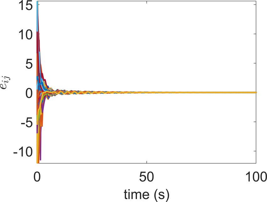
we consider all robots. Define F := diag{f10 , . . . , fN
                                                        0
                                                          } ∈          (approximately) represent many different robotic systems in
  nN ×N                                      nN ×nN
R       , K := diag{K1 , . . . , KN } ∈ R                 and          reality; thus, the design methodology is widely applicable.
Φ := (Φ> 1 , · · · , Φ> >
                      N ) . Then we have                                  Different from the unicycle model, which allows backward
                                                                       or stationary motion, we use the following Dubins-car-like
               Φ̇ = −KΦ − FF> KΦ − kc Fc(w).                 (9)
                                                                       3D model that describes fixed-wing aircraft dynamics:
One can also calculate that ẇi = 0 · · · 0 1 ( χi (ξi )+
                                                   pf
                                                                           ṗi1 = v cos θi , ṗi2 = v sin θi , ṗi3 = uzi , θ˙i = uθi ,         (12)
kc co χi (ξi )) = (−1)n +fi0 (wi )> Ki Φi (ξi )+kc ci (w). There-
fore, we have that                                                     where v is a constant airspeed, (pi1 , pi2 , pi3 )> ∈ R3 is the
                  ˙ = (−1)n 1 + F> KΦ − kc Lw̃,
                 w̃                                           (10)     position of the i-th aircraft’s center of mass, θi is the yaw
                                                                       angle, and uzi and uθi are two control inputs to be designed.
                  N
where 1 ∈ R is a vector consisting of all ones. The                    Since the essential role of a guiding vector field is to provide
Laplacian matrix can be re-written as L = DD> , where                  the desired yaw angle to guide the flight of a fixed-wing
D ∈ RN ×|E| is the incidence matrix. We define the composite           aircraft, the core idea behind the control algorithm design is
error vector e := (Φ> , (D> w̃)> )> ∈ RnN +|E| and the                 to align the aircraft’s flying direction with that given by the
composite gain matrix to be K := diag{K, kc I|E| } ∈                   guiding vector field. To this end, as the guiding vector field has
R(nN +|E|)×(nN +|E|) , where Im is the |E|-by-|E| identity             an additional coordinate, one needs to add an additional virtual
matrix. Therefore, from (8), (9) and (10), and noting that             coordinate pi4 such that the aircraft’s generalized position
D> 1 = 0, we have the following composite error dynamics:              is (pi1 , pi2 , pi3 , pi4 ) ∈ R4 . Correspondingly, its generalized

              Φ̇

                      −KΦ − FF> KΦ + kc FLw̃
                                                                      velocity is (ṗi1 , ṗi2 , ṗi3 , ṗi4 ) = (v cos θi , v sin θi , uzi , ṗi4 ),
      ė =       ˙  =   > >          >         .              (11)     where ṗi4 is virtual and extra design freedom. To align the
             D> w̃     D F KΦ − kc D Lw̃
                                                                       aircraft heading v(cos θi , sin θi ) with the counterpart of the
Theorem 1. The coordinating vector fields Xi for i ∈ ZN   1            coordinating vector field Xi , we need to “partially normalize”
designed by combining (3), (4), (5) and (7) solve Problem 1            the vector field Xi such that its first two entries p      form a vector
globally in the sense that the initial states ξ0 ∈ R(n+1)×N            of the same length as v; that is, vXi := vXi / X2i1 + X2i2 .
can be chosen arbitrarily.                                             Subsequently, we design the yaw angular control input uθi
Proof. The proof is in the extended version [47].                      such that the aircraft heading v(cos θi , sin θi ) aligns gradually
                                                                       with the vector formed by the first two entries of vXi (i.e.,
Remark 2. Our work’s focus is the distributed control algo-            v(Xi1 , Xi2 )). For the last two entries of the generalized
rithm based on guiding vector fields, so collision avoidance           velocity (ṗi1 , ṗi2 , ṗi3 , ṗi4 ), one can simply equate them with
is not elaborated here. However, our proposed approach can             those of vXi , respectively:
incorporate existing collision avoidance algorithms [48], [49].                               q                                 q
For example, we can modify the nominal guiding vector                   ṗi3 = uzi = vXi3 /    X2i1 + X2i2 ,    ṗi4 = vXi4 /    X2i1 + X2i2 . (13)
field (5) in a minimally invasive way using safety barrier
certificates [49], [50]. Specifically, we add an extra term            The control algorithm design method [36], [54] is extended
ucol   ∈ Rn+1 to the vector field in (5), and this term is             here to handle the issue with the actuator saturation in the
  i
calculated by a quadratic program min ucol
                                                          2            yaw control input uθi as described below. First, we define
                                                  i (t)      subject
                                                                       the saturation function Satba : R → R by Satba (x) = x for
to the constraints Ḃij (ξi , ξj ) ≤ 1/Bij (ξi , ξj ) for j 6= i and
                                                                       x ∈ [a, b], Satba (x) = a for x ∈ (−∞, a) and Satba (x) = b
i, j ∈ ZN1 , where Bij (ξi , ξj ) is a control barrier function
                                             2                         for x ∈ (b, ∞), where a, b ∈ R, a < b are some constants.
[51] (e.g., Bij (ξi , ξj ) = 1/(kpi − pj k − R2 ), where pi
                                                                       The saturation function Satba is Lipschitz continuous. For
is the physical position and R is the safe distance between
                                                                       convenience, we call the time interval when Satba (x(t)) =
robots). The collision avoidance behavior is shown in the
                                                                       b the upper saturation period, and the time interval when
supplementary video, but the theoretical analysis is left for
                                                                       Satba (x(t)) = a the lower saturation period. We use v to
future work.                                                       /
                                                                       denote the normalization of a vector v (i.e., v = v/ kvk). We
   IV. C ONTROLLER FOR A D UBINS - CAR - LIKE MODEL                    also define Xpi = (Xi1 , Xi2 )> , which is the vector formed
   If a robot’s motion can be approximately modeled by the             by the first two entries of the normalized vector field Xi .
single-integrator model, then the coordinating vector field in         One can easily calculate that Xpi = (Xi1 , Xi2 ). Therefore,
(5) can be used directly as the velocity input to the robot.           Xpi represents the orientation given by the vector field Xi .
For the unicycle model, one can use feedback linearization                Suppose we are given 3D physical desired paths Piphy ⊆
                                                                         3
to transform it into the single-integrator model [52] to utilize       R parameterized by (2), and the coordinating vector field
the guiding vector field directly. However, we will design a           Xi : R3+N → R3+1 in (5). We denote hi = hi =
controller for unicycles traveling at a constant speed (i.e., the      (cos θi , sin θi )> as the orientation of the aircraft, the (signed)
                                                                                                             p
Dubins-car model) without using the feedback linearization             angle difference directed from X         to hi by σi ∈ (−π, π] and
                                                                                                           0i −1
technique. Note that the control algorithm design idea in this         define the rotation matrix E = 1 0 . Then after introducing
section is applicable to robot models of which the motions are         another natural assumption, one can reach Theorem 2 showing
characterized by the robot’s orientations, such as the car-like        that the aircraft’s orientation hi will converge to that of the
model and the underwater glider model [53]. These models               vector field Xpi asymptotically (i.e., σi converges to zero).
even if it temporarily deviates from the desired path due
to saturation or other constraints (such as path curvature),
as long as the vector field orientation change rate1 θ̇id does
not saturate the control input persistently. The subsequent
fixed-wing aircraft experiment verifies the effectiveness of
the control law. Nevertheless, we can remove Condition 2 in
Theorem 2 by imposing an upper bound on the magnitude of
θ̇id . Due to the page limit, the detail is in the extended version
[47]. To reduce |θ̇id | and avoid possible saturation, one can
scale down the path parameter in the parametric functions in
(2) (e.g. by changing fij (wi ) to fij (βwi ), where 0 < β < 1),
or choose another desired path with a smaller curvature.
Another solution is to impose an additional constraint |uθi | ≤
min{|a|, |b|} on the quadratic program mentioned in Remark
2.
Remark 3. Theorem 2 guarantees that each robot’s moving
p The path is parameterized by xi1 =
Fig. 1. The first simulation results.
direction will align with the vector field eventually. Therefore,
15 sin(2wi ), xi2 = 30 sin(wi ) 0.5(1 − 0.5 sin2 (wi )) and xi3 = 5 +
5 cos(2wi ) − 2 for all i ∈ ZN 1 . The period of this closed curve is T = 2π
it can be shown that the convergence results of the robots’
and the desired differences between two adjacent robots’ virtual coordinates trajectories are the same as the integral curves of the guiding
are T /(2N ). The desired relative states ∆ij are constructed from the vector field in (6). The rigorous theoretical analysis relies on
reference wi∗ = (i − 1)T /(2N ) for i ∈ ZN 1 . The control gains are: ki1 =
ki2 = ki3 = 1, kc = 300 for i ∈ ZN the input-to-state stability (ISS) property [56, Chapter 4.9],
1 , where kc is large to accelerate the
motion coordination. On top, the trajectories of robots, where squares and and is left for future work. /
circles symbolize the trajectories’ initial and final positions, respectively. On
the bottom left, the path-following errors eij for i ∈ ZN n
1 and j ∈ Z1 . On V. S IMULATIONS AND E XPERIMENTS
the bottom right, the coordination error wi − wj − ∆ij for i, j ∈ ZN 1 i < j.
,
A. Simulations
Assumption 3. The desired paths can be traveled by robots We use cycle graphs as the communication topology, and
with saturated angular velocity, and the eventual coordination thus each robot is only allowed to communicate with its
is feasible [55]. two adjacent neighbors. This simple communication graph
This assumption is reasonable. It restricts the design of results in very low communication and computation load.
the desired path and the reference state vector ω ∗ (hence In the first simulation, we let N = 50 robots follow a 3D
∆∗ ) to guarantee the feasibility of the robot motions, and self-intersecting bent “∞”-shaped curve. As shown in Fig.
avoid the collision of robots in the steady-state, respectively. 1, all robots follow the “∞”-shaped path successfully and
For example, if the parametric desired path is periodic and keep desired positions (in terms of wi ) between each other.
closed, then one can simply choose ∆ij = T /N , where T is In the second simulation, we employ N = 3 robots to show
the period, for any two neighboring indices i, j ∈ ZN 1 .
that our algorithm is applicable for complicated and open
curves (i.e., aperiodic curve), and demonstrate its potential
Theorem 2. Assume that the vector field satisfies Xi1 (ξi )2 + application to volume coverage in 3D (see Fig. 2). In the
Xi2 (ξi )2 > γ > 0 for ξi ∈ R3+1 , i ∈ ZN 1 , where γ is a third simulation, we show how different robots can follow
positive constant. Let the angular velocity control input uθi different desired paths while still coordinating their motions
>
in model (12) be θ˙i = uθi = Satba (θ̇id − kθ hi EXpi ), where to form some (time-varying) formation shapes (see Fig. 3).
> p
θ̇id = −Xpi E Ẋi / kXpi k, kθ > 0 is a constant, and a < 0,
b > 0 are constants for the saturation function Satba . If the B. Flights with fixed-wing aircraft
angle difference σi satisfies the following conditions: In this experiment, two autonomous fixed-wing aircraft (i.e.,
1) The initial angle difference σi (t = 0) 6= π; Autonomous Opterra 1.2m) similar to [5], [57] are employed
2) σi (t) ∈ [0, π) during the upper saturation period, and to validate Theorem 2. The aircraft are equipped with the open-
σi (t) ∈ (−π, 0] during the lower saturation period, source software/hardware project Paparazzi [58]. The codes
related to the proposed algorithm are in [59]. We choose the
then σi will vanish asymptotically (i.e., σi (t) → 0).
following 3D Lissajous curve f1 (w) = 225 cos(w), f2 (w) =
Proof. The proof is in the extended version [47]. 225 cos(2w + π/2), f3 (w) = −20 cos(2w), which is a bent
“∞”-shaped path. The mission requires both aircraft to have
Although Condition 2 in Theorem 2 might be difficult
∆12 = 0; i.e., to fly in a tight formation. The collision is
to check in practice, it conveys the core message that the
avoided by biasing the GPS measurement of one aircraft by a
saturation, albeit allowed, should not last for a long time.
constant distance of 1m in the horizontal plane; i.e., when the
However, this condition is only sufficient, while in practice,
violating this condition does not immediately entail instability 1 As X˙p = θ̇ d EXp , and EXp is orthogonal to Xp , the term θ̇ d in (2)
i i i i i i
of the algorithm. As the aircraft is guided by the vector field, encodes how fast the vector field changes its orientation along the trajectory
the aircraft can re-orient its heading towards the desired path of the aircraft (i.e., θ̇id is the vector field orientation change rate).Time = 97 Time = 160
100 100
80 80
60 60
40 40
20 20
0 0
200 200
100 100
0 0
−100 −100
−100 0 100 −200 −100 0 100 −200
200 300 −300 200 300 −300
Time = 185 Time = 372
100 100
80 80
Fig. 2. The second simulation results. We choose a 3D Lissajous curve with 60 60
irrational coefficients: xi1 = cos(nx wi ) + mx , xi2 √ = cos(ny wi ) + my 40 40
20 20
and xi3 = cos(nz wi )+mz for i ∈ ZN 1 , where nx = 2, ny = 4.1, nz = 0
200
0
200
100 100
7.1, mx = 0.1, my = 0.7, mz = 0. This is an open curve bounded in a 0
−100
0
−100
−100 0 −200 −100 0 −200
cube (as nx is irrational). Therefore, it is ideal for a volume coverage task. 100 200 300 −300 100 200 300 −300
The control gains for the coordinating vector field are: ki1 = ki2 = ki3 =
kc = 1 for i ∈ ZN 1 . Squares and circles symbolize trajectories’ initial and Fig. 4. Two aircraft (blue and red trajectories) flying together tracking a 3D
final positions, and the solid blue lines are the trajectories during the last 30 bent “∞”-shaped path. Although we show that the positions are overlapped,
time steps. The first sub-figure shows the trajectories of three robots (red the same position corresponds to two different ones in reality since their
curves). The magenta curve represents part of the Lissajous curve. The last GPS receptors are biased with respect to each other by around 1 meter in
two sub-figures correspond to the Y-Z side views of the trajectories for 9.4 the XY plane.
and 76.8 seconds, respectively.
φ1 [m] (x) φ2 [m] (y) φ3 [m] (z) ew [rads]
2 0.50
0
0 0.25
0
0.00
−20
−2
−5 −0.25
−4
200 400 200 400 200 400 200 400
Fig. 5. Distance errors (in XYZ) of the two aircraft (blue and red) to
the desired 3D path, and errors with respect to the desired ∆w = 0. The
horizontal axes denote time in seconds.
aircraft are not equipped with the required sensors or actuators
(e.g., spoilers/flaps while descending), and the wind always
Fig. 3. The third simulation results. We let N = 21 robots follow three
different paths, where the first seven robots follow a large circle of radius
affects the speed of the airplane. By contrast, our guidance
a = 10, the last seven robots follow a small circle of radius b = 5, and algorithm is free from such a requirement since the parameter
the remaining seven robots follow an ellipse with the semimajor axis a and w is in a closed-loop with the aircraft state, and thereby
the semiminor axis b. The robots are distributed evenly in the path through
the parameter wi ; i.e., we construct the desired relative states ∆ij from
adapting automatically to the position and velocity of the
the references wi∗ (t) = (i − 1)2π/N , for i ∈ ZN 1 . The control gains are:
aircraft.
ki1 = ki2 = 1, kc = 100 for all i ∈ ZN 1 , where the large value is chosen
for kc to accelerate the motion coordination. The squares and ∗ symbolize
the trajectories’ initial and final positions, respectively. The dashed black line VI. C ONCLUSIONS AND FUTURE WORK
shows the communication links between robots and the resulting formation
shape. During the steady-state, these robots do not collide into one another,
since the distributed coordination guarantees that the adjacent neighbors We design a coordinating vector field for multiple robots to
satisfy |wi − wj | = 2π/N , where i and j are any neighboring indices. follow (possibly different) desired paths while coordinating
their motions distributedly, and a control algorithm is designed
aircraft achieve ∆12 = 0, they are displaced physically. We for the Dubins-car-like model. In particular, we use the
choose k1 = k2 = 0.002, k3 = 0.0025, kc = 0.01, kθ = 1, path parameter wi as an additional virtual coordinate for
and the communication frequency is 10 Hz. In the experiment, the guiding vector field, which is further utilized as local
the weather forecast reported 14 degrees Celsius and a South information communicated among neighboring robots to
wind of 10 km/h. In Figure 4, the telemetry shows that both achieve motion coordination. The vector field is rigorously
airplanes converge to fly together while following the path. proved to enable robots to follow their respective desired
The experiment shows that once an aircraft goes faster than paths while coordinating their motions. Our algorithm is a
its partner, the algorithm guides the airplane to deviate from significant extension of the circumnavigation algorithms and
the curve to travel more distances to “wait” for its partner. circular formation control algorithms since it enables multiple
Nevertheless, these deviations from the desired path are within robots to cooperatively move along arbitrary paths and form
the order of one or two meters (see Figure 5). different (possibly varying) desired shapes. Moreover, our
Note that the employed aircraft do not control their ground algorithm requires a very low amount of local communication.
speeds. In fact, they have a reference signal in their throttle to Simulations and experiments support the theoretical results.
keep a safe airspeed, and the aircraft increase/decrease such Future work includes detailed analysis of the collision
a reference to ascend/descend while following the 3D path. avoidance using control barrier functions, and performance
A traditional trajectory tracking algorithm would force the evaluation in the presence of localization errors. We will
aircraft to track an open-loop f1 (t), f2 (t) and f3 (t); i.e., it compare our algorithm with the approaches mentioned in the
requires controlling the airspeed/ground speed of the aircraft. Introduction in our future work, and will also consider the
Such a requirement is demanding (or unsatisfiable) if the problem on smooth manifolds.R EFERENCES [22] ——, “Forming circle formations of anonymous mobile agents with
order preservation,” IEEE Transactions on Automatic Control, vol. 58,
[1] G.-Z. Yang, J. Bellingham, P. E. Dupont, P. Fischer, L. Floridi, R. Full, no. 12, pp. 3248–3254, 2013.
N. Jacobstein, V. Kumar, M. McNutt, R. Merrifield et al., “The grand [23] R. Sepulchre, D. A. Paley, and N. E. Leonard, “Stabilization of planar
challenges of science robotics,” Science robotics, vol. 3, no. 14, p. collective motion: All-to-all communication,” IEEE Transactions on
7650, 2018. Automatic Control, vol. 52, no. 5, pp. 811–824, 2007.
[2] T. I. Fossen, M. Breivik, and R. Skjetne, “Line-of-sight path following [24] J. Fonseca, J. Wei, K. H. Johansson, and T. A. Johansen, “Coopera-
of underactuated marine craft,” IFAC Proceedings Volumes, vol. 36, tive decentralized circumnavigation with application to algal bloom
no. 21, pp. 211–216, 2003. tracking,” arXiv preprint arXiv:1903.05993, 2019.
[3] P. B. Sujit, S. Saripalli, and J. B. Sousa, “Unmanned aerial vehicle [25] I. Shames, S. Dasgupta, B. Fidan, and B. D. O. Anderson, “Cir-
path following: A survey and analysis of algorithms for fixed-wing cumnavigation using distance measurements under slow drift,” IEEE
unmanned aerial vehicless,” IEEE Control Systems, vol. 34, no. 1, pp. Transactions on Automatic Control, vol. 57, no. 4, pp. 889–903, 2011.
42–59, Feb 2014. [26] M. Deghat, I. Shames, B. D. O. Anderson, and C. Yu, “Localization
[4] Y. A. Kapitanyuk, A. V. Proskurnikov, and M. Cao, “A guiding vector- and circumnavigation of a slowly moving target using bearing mea-
field algorithm for path-following control of nonholonomic mobile surements,” IEEE Transactions on Automatic Control, vol. 59, no. 8,
robots,” IEEE Transactions on Control Systems Technology, vol. 26, pp. 2182–2188, 2014.
no. 4, pp. 1372–1385, July 2018. [27] R. Zheng and D. Sun, “Circumnavigation by a mobile robot using
[5] H. G. De Marina, Z. Sun, M. Bronz, and G. Hattenberger, “Circular bearing measurements,” in 2014 IEEE/RSJ International Conference
formation control of fixed-wing UAVs with constant speeds,” in 2017 on Intelligent Robots and Systems. IEEE, 2014, pp. 4643–4648.
IEEE/RSJ International Conference on Intelligent Robots and Systems [28] W. Yao, H. Lu, Z. Zeng, J. Xiao, and Z. Zheng, “Distributed static
(IROS). IEEE, 2017, pp. 5298–5303. and dynamic circumnavigation control with arbitrary spacings for a
[6] K. Nakai and K. Uchiyama, “Vector fields for UAV guidance using heterogeneous multi-robot system,” Journal of Intelligent & Robotic
potential function method for formation flight,” in AIAA Guidance, Systems, vol. 94, no. 3-4, pp. 883–905, 2019.
Navigation, and Control (GNC) Conference, 2013, p. 4626. [29] W. Yao, Z. Zeng, X. Wang, H. Lu, and Z. Zheng, “Distributed
[7] L. C. Pimenta, G. A. Pereira, M. M. Gonçalves, N. Michael, M. Turpin, encirclement control with arbitrary spacing for multiple anonymous
and V. Kumar, “Decentralized controllers for perimeter surveillance mobile robots,” in 2017 36th Chinese Control Conference (CCC).
with teams of aerial robots,” Advanced Robotics, vol. 27, no. 9, pp. IEEE, 2017, pp. 8800–8805.
697–709, 2013. [30] W. Yao, S. Luo, H. Lu, and J. Xiao, “Distributed circumnavigation
[8] J. Ghommam, H. Mehrjerdi, M. Saad, and F. Mnif, “Formation control with dynamic spacing for a heterogeneous multi-robot system,”
path following control of unicycle-type mobile robots,” Robotics and in Robot World Cup. Springer, 2018, pp. 374–386.
Autonomous Systems, vol. 58, no. 5, pp. 727–736, 2010. [31] J. Ma, W. Yao, W. Dai, H. Lu, J. Xiao, and Z. Zheng, “Cooperative
[9] H. Chen, Y. Cong, X. Wang, X. Xu, and L. Shen, “Coordinated encirclement control for a group of targets by decentralized robots
path-following control of fixed-wing unmanned aerial vehicles,” IEEE with collision avoidance,” in 2018 37th Chinese Control Conference
Transactions on Systems, Man, and Cybernetics: Systems, 2021. (CCC). IEEE, 2018, pp. 6848–6853.
[10] Y. Lan, G. Yan, and Z. Lin, “Synthesis of distributed control of coor- [32] H. Lu, W. Yao, and L. Chen, “Distributed multi-robot circumnavigation
dinated path following based on hybrid approach,” IEEE Transactions with dynamic spacing and time delay,” Journal of Intelligent & Robotic
on Automatic Control, vol. 56, no. 5, pp. 1170–1175, 2011. Systems, pp. 1–18, 2019.
[11] Y. Wang, D. Wang, and S. Zhu, “Cooperative moving path following for [33] A. H. Mong-ying and V. Kumar, “Pattern generation with multiple
multiple fixed-wing unmanned aerial vehicles with speed constraints,” robots,” in Proceedings 2006 IEEE International Conference on
Automatica, vol. 100, pp. 82–89, 2019. Robotics and Automation (ICRA). IEEE, 2006, pp. 2442–2447.
[12] M. Burger, A. Pavlov, E. Borhaug, and K. Y. Pettersen, “Straight [34] A. H. Mong-ying, S. Loizou, and V. Kumar, “Stabilization of multiple
line path following for formations of underactuated surface vessels robots on stable orbits via local sensing,” in Proceedings 2007 IEEE
under influence of constant ocean currents,” in 2009 American Control International Conference on Robotics and Automation (ICRA). IEEE,
Conference. IEEE, 2009, pp. 3065–3070. 2007, pp. 2312–2317.
[13] A. Doosthoseini and C. Nielsen, “Coordinated path following for [35] M. Mesbahi and M. Egerstedt, Graph theoretic methods in multiagent
unicycles: A nested invariant sets approach,” Automatica, vol. 60, pp. networks. Princeton University Press, 2010, vol. 33.
17–29, 2015. [36] W. Yao, H. G. de Marina, B. Lin, and M. Cao, “Singularity-free guiding
[14] L. A. V. Reyes and H. G. Tanner, “Flocking, formation control, and vector field for robot navigation,” IEEE Transactions on Robotics,
path following for a group of mobile robots,” IEEE Transactions on vol. 37, no. 4, 2021.
Control Systems Technology, vol. 23, no. 4, pp. 1268–1282, 2015. [37] W. Yao, Y. A. Kapitanyuk, and M. Cao, “Robotic path following in
[15] F. Zhang and N. E. Leonard, “Coordinated patterns of unit speed 3D using a guiding vector field,” in IEEE Conference on Decision and
particles on a closed curve,” Systems & control letters, vol. 56, no. 6, Control, 2018, pp. 4475–4480.
pp. 397–407, 2007. [38] V. M. Gonçalves, L. C. A. Pimenta, C. A. Maia, B. C. O. Dutra, and
[16] L. Sabattini, C. Secchi, M. Cocetti, A. Levratti, and C. Fantuzzi, “Im- G. A. S. Pereira, “Vector fields for robot navigation along time-varying
plementation of coordinated complex dynamic behaviors in multirobot curves in n-dimensions,” IEEE Transactions on Robotics, vol. 26, no. 4,
systems,” IEEE Transactions on Robotics, vol. 31, no. 4, pp. 1018–1032, pp. 647–659, Aug 2010.
2015. [39] D. A. Lawrence, E. W. Frew, and W. J. Pisano, “Lyapunov vector fields
[17] M. Iqbal, S.-i. Azuma, J. Leth, and T. D. Ngo, “Circular and concentric for autonomous unmanned aircraft flight control,” Journal of Guidance,
formation of kinematic unicycles,” in 2019 International Conference Control, and Dynamics, vol. 31, no. 5, pp. 1220–1229, 2008.
on Robotics and Automation (ICRA). IEEE, 2019, pp. 1–6. [40] W. Yao and M. Cao, “Path following control in 3D using a vector
[18] D. St-Onge, C. Pinciroli, and G. Beltrame, “Circle formation with field,” Automatica, vol. 117, p. 108957, 2020.
computation-free robots shows emergent behavioural structure,” in [41] W. Yao, B. Lin, B. D. O. Anderson, and M. Cao, “Topological
2018 IEEE/RSJ International Conference on Intelligent Robots and analysis of vector-field guided path following on manifolds,” 2020,
Systems (IROS). IEEE, 2018, pp. 5344–5349. submitted. [Online]. Available: http://tiny.cc/yao topo
[19] S. Zhu, D. Wang, and C. B. Low, “Cooperative control of multiple [42] A. Galbis and M. Maestre, Vector analysis versus vector calculus.
UAVs for moving source seeking,” Journal of Intelligent & Robotic Springer Science & Business Media, 2012.
Systems, vol. 74, no. 1-2, pp. 333–346, 2014. [43] W. Yao, H. G. de Marina, and M. Cao, “Vector field guided path
[20] Z. Sun, H. G. de Marina, G. S. Seyboth, B. D. O. Anderson, and following control: Singularity elimination and global convergence,” in
C. Yu, “Circular formation control of multiple unicycle-type agents 2020 59th IEEE Conference on Decision and Control (CDC). IEEE,
with nonidentical constant speeds,” IEEE Transactions on Control 2020, pp. 1543–1549.
Systems Technology, vol. 27, no. 1, pp. 192–205, 2018. [44] D. R. Nelson, D. B. Barber, T. W. McLain, and R. W. Beard, “Vector
[21] C. Wang, G. Xie, and M. Cao, “Controlling anonymous mobile field path following for miniature air vehicles,” IEEE Transactions on
agents with unidirectional locomotion to form formations on a circle,” Robotics, vol. 23, no. 3, pp. 519–529, 2007.
Automatica, vol. 50, no. 4, pp. 1100–1108, 2014. [45] H. G. de Marina, “Maneuvering and robustness issues in undirecteddisplacement-consensus-based formation control,” IEEE Transactions
on Automatic Control, 2020.
[46] W. Ren and R. W. Beard, Distributed consensus in multi-vehicle
cooperative control. Springer, 2008, vol. 27, no. 2.
[47] W. Yao, H. G. de Marina, Z. Sun, and M. Cao, “Guiding vector fields
for multi-robot coordinated navigation,” 2021, in preparation.
[48] W. Yao, B. Lin, and M. Cao, “Integrated path following and collision
avoidance using a composite vector field,” in 2019 IEEE 58th
Conference on Decision and Control (CDC). IEEE, 2019, pp. 250–255.
[49] L. Wang, A. D. Ames, and M. Egerstedt, “Safety barrier certificates
for collisions-free multirobot systems,” IEEE Transactions on Robotics,
vol. 33, no. 3, pp. 661–674, 2017.
[50] ——, “Safe certificate-based maneuvers for teams of quadrotors
using differential flatness,” in 2017 IEEE International Conference on
Robotics and Automation (ICRA). IEEE, 2017, pp. 3293–3298.
[51] A. D. Ames, S. Coogan, M. Egerstedt, G. Notomista, K. Sreenath,
and P. Tabuada, “Control barrier functions: Theory and applications,”
in 2019 18th European Control Conference (ECC). IEEE, 2019, pp.
3420–3431.
[52] X. Yun and Y. Yamamoto, “On feedback linearization of mobile
robots,” Department of Computer and Information Science, University
of Pennsylvania, technical report, 1992.
[53] B. Siciliano and O. Khatib, Springer Handbook of Robotics. Secaucus,
NJ, USA: Springer-Verlag New York, Inc., 2007.
[54] A. M. Rezende, V. M. Gonçalves, G. V. Raffo, and L. C. Pimenta,
“Robust fixed-wing UAV guidance with circulating artificial vector
fields,” in 2018 IEEE/RSJ International Conference on Intelligent
Robots and Systems (IROS). IEEE, 2018, pp. 5892–5899.
[55] L. J. Colombo and D. V. Dimarogonas, “Motion feasibility conditions
for multiagent control systems on Lie groups,” IEEE Transactions on
Control of Network Systems, vol. 7, no. 1, pp. 493–502, 2019.
[56] H. Khalil, Nonlinear Systems, 3rd ed. Prentice Hall, 2002.
[57] Y. A. Kapitanyuk, H. G. de Marina, A. V. Proskurnikov, and M. Cao,
“Guiding vector field algorithm for a moving path following problem,”
IFAC-PapersOnLine, vol. 50, no. 1, pp. 6983–6988, 2017.
[58] B. Gati, “Open source autopilot for academic research-the paparazzi
system,” in 2013 American Control Conference. IEEE, 2013, pp.
1478–1481.
[59] “Code repository for this paper,” 2020. [Online]. Avail-
able: https://github.com/noether/paparazzi/tree/gvf param multi/sw/
airborne/modules/guidance/gvf parametricYou can also read