Tropical Cyclone Winds from WindSat, AMSR2, and SMAP: Comparison with the HWRF Model
←
→
Page content transcription
If your browser does not render page correctly, please read the page content below
remote sensing
Article
Tropical Cyclone Winds from WindSat, AMSR2, and SMAP:
Comparison with the HWRF Model
Andrew Manaster *, Lucrezia Ricciardulli and Thomas Meissner

                                          Remote Sensing Systems, 444 Tenth Street, Suite 200, Santa Rosa, CA 95401, USA; ricciardulli@remss.com (L.R.);
                                          meissner@remss.com (T.M.)
                                          * Correspondence: manaster@remss.com

                                          Abstract: A new data set of tropical cyclone winds (‘TC-winds’) through rain as observed by the
                                          WindSat and AMSR2 microwave radiometers has been developed by making use of a linear combi-
                                          nation of C- and X-band frequency channels. These winds, along with tropical cyclone winds from
                                          the SMAP L-band radiometer, are compared with the Hurricane Weather Research and Forecasting
                                          (HWRF) model. Due to differences in spatial scales between the satellites and the high-resolution
                                          HWRF model, resampling must be performed on the model winds before comparisons are done.
                                          Various ways of spatial resampling are discussed in detail, and an optimal method is determined.
                                          Additionally, resampled model winds must be temporally interpolated to the time of the satellite
                                          before direct comparisons are made. This interpolation can occasionally result in un-physical 2D
                                          wind fields, especially for fast-moving storms. To assist users with this problem, a methodology for
                                          handling un-physical wind features is detailed. Results of overall comparisons between the satellites
                                          and HWRF for 19 storms between 2017 and 2020 displayed consistent storm features, with overall

                                          average biases less than 1 m/s and standard deviations below 4 m/s for all tropical cyclone winds
                                   between 10 and 60 m/s. Differences were seen when the comparisons were performed separately
Citation: Manaster, A.; Ricciardulli,     for the Atlantic and Pacific basins, with biases and standard deviations between the satellites and
L.; Meissner, T. Tropical Cyclone         HWRF showing better agreement in the Atlantic. The impact of rain on the satellite wind retrievals is
Winds from WindSat, AMSR2, and            discussed, and no systematic bias was seen between the three sensors, despite the fact that they use
SMAP: Comparison with the HWRF            different frequency channels in their tropical cyclone winds-through-rain retrieval algorithms.
Model. Remote Sens. 2021, 13, 2347.
https://doi.org/10.3390/rs13122347        Keywords: microwave radiometers; tropical cyclones; winds

Academic Editor:
Vladimir N. Kudryavtsev

                                          1. Introduction
Received: 10 May 2021
Accepted: 11 June 2021
                                               Passive satellite microwave radiometers, which operate at frequencies in the C-band
Published: 16 June 2021
                                          (4–8 GHz) or higher, have historically had difficulty measuring oceanic surface winds
                                          in areas of heavy precipitation [1–3]. This is due to the fact that raindrops attenuate the
Publisher’s Note: MDPI stays neutral
                                          observed signal coming from the surface. In addition, it is difficult to distinguish the signals
with regard to jurisdictional claims in
                                          caused by wind roughening of the ocean surface from those due to rain. The attenuation
published maps and institutional affil-   can degrade the satellite retrievals to the point where they are not useable for scientific
iations.                                  purposes. This can often lead to gaps in microwave-satellite coverage when precipitation
                                          is present, particularly in tropical cyclones, which are often affected by heavy precipitation.
                                          However, it is possible to mitigate the problem of rain attenuation for microwave sensors
                                          that operate at the C- and X-band (8–12 GHz) frequencies by using a linear combination of
Copyright: © 2021 by the authors.
                                          these channels that is simultaneously sensitive to wind speed and relatively insensitive
Licensee MDPI, Basel, Switzerland.
                                          to rain [4]. This is due to the fact that the effect of atmospheric scattering is still relatively
This article is an open access article
                                          small at these frequencies [5], and the spectral differences in brightness temperature (TB)
distributed under the terms and           due to wind induced surface emissivity between the two channels are relatively small,
conditions of the Creative Commons        while the spectral differences due to rain attenuation are relatively large.
Attribution (CC BY) license (https://          Recently, an algorithm [4] was developed for the AMSR2, AMSR-E, and WindSat ra-
creativecommons.org/licenses/by/          diometers that takes advantage of their C- and X-band channels to measure winds in tropi-
4.0/).                                    cal cyclones, even in areas of heavy precipitation (see [6–9] for a further description of these

Remote Sens. 2021, 13, 2347. https://doi.org/10.3390/rs13122347                                       https://www.mdpi.com/journal/remotesensing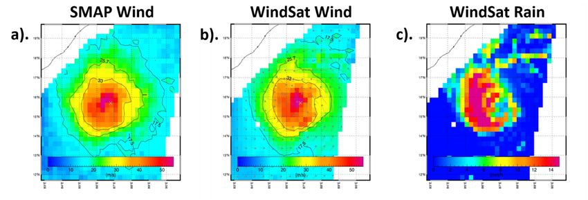
Remote Sens. 2021, 13, 2347                                                                                            2 of 19

                              instruments). This algorithm was trained using the Soil Moisture Active Passive (SMAP)
                              L-band (1.4 GHz) radiometer, which was launched by NASA in 2015 [10–12]. SMAP and
                              other L-band radiometers, such as the Soil Moisture and Ocean Salinity (SMOS [13,14])
                              radiometer, have several advantages over other microwave sensors when making wind
                              measurements in tropical cyclones. First, due to the low frequency of their observed signal,
                              L-band radiometers are minimally affected by rain, and can retrieve surface winds unob-
                              structed [13,15]. Secondly, the surface brightness temperature (TB) signal measured by
                              L-band radiometers increases approximately linearly with wind speed and does not satu-
                              rate at higher winds. This allows L-band radiometers to make accurate wind measurements
                              up to 70 m/s (Category 5 tropical storms) without signal degradation [10,13,14,16–19]. Be-
                              cause of this, SMAP is an ideal candidate to help train algorithms for both the WindSat and
                              AMSR radiometers, as detailed in [4].
                                    These new algorithms have resulted in the creation of new wind products referred to
                              as ‘TC-winds’, which were developed and processed by Remote Sensing Systems (RSS)
                              for the AMSR-E, AMSR2, WindSat, and SMAP radiometers. TC-winds are processed in
                              near-real time, with ~3 h latency for AMSR2 and SMAP, and are freely distributed to the
                              public. The combined measurements from SMAP and AMSR2 provide very good spatial
                              and temporal coverage in the tropics. As such, these TC-winds constitute an important
                              data set for characterizing tropical cyclone intensity, shape, and structure throughout the
                              course of a storm’s lifetime. These satellite wind measurements offer valuable information
                              when assimilated into tropical cyclone forecast models such as the US Navy’s Automated
                              Tropical Cyclone Forecasting System (ATCF) [20]. These assimilated data take the form of
                              tropical cyclone fixes, which include the maximum 10 min maximum sustained winds and
                              wind radii for the 34 kt (17 m/s), 50 kt (25 m/s), and 64 kt (33 m/s) winds for each satellite
                              pass over a TC in all tropical ocean basins.
                                    Due to their wide range of scientific applications, it is important to assess the quality
                              of the TC-winds by comparing them with reliable external sources. This study’s companion
                              paper [4] performed a case study that computed intensity (maximum wind speed) and radii
                              of several selected TCs using the TC-winds and compared them with the storm parameters
                              derived from operational storm forecasts and analyses.
                                    Our study aims to build on the results presented in [4] by comparing the TC-winds
                              with surface wind fields from the Hurricane Weather Research and Forecasting (HWRF)
                              model, a high-resolution operational storm forecast model that is routinely tested, evalu-
                              ated, and upgraded [21–25]. The HWRF model provides an external data source to compare
                              to the satellites for each tropical cyclone of interest. However, before direct comparisons
                              between the TC-winds and HWRF can be performed, two preliminary steps are necessary:
                              (1) the high resolution HWRF model must be resampled to a coarser resolution similar to
                              that of the satellites so that the features resolved by HWRF are similar to those of the satel-
                              lite radiometers, and (2) the HWRF winds at the model output times must be temporally
                              interpolated to the time of the satellite overpass. Both of these steps are integral parts of
                              the study and are discussed in greater detail later in this paper.
                                    The paper is organized as follows: Section 2 describes the data sets used in this study
                              and provides a brief additional assessment of the performance of TC-winds presented
                              in [4]. Section 3 describes the methodology for resampling the HWRF model to the same
                              resolution as the satellites. This section also discusses temporal interpolation and how
                              to address pitfalls associated with it. Section 4 presents the results of the comparison
                              after the HWRF data were appropriately resampled and interpolated. Differences in the
                              satellite-model comparisons between different ocean basins and the impact of rain are
                              discussed. Section 5 concludes and summarizes the work.

                              2. Data Sets
                              2.1. SMAP Winds
                                  Since 2017, RSS has been producing SMAP wind data in the form of twice-daily
                              gridded maps (for ascending and descending swaths) on a 0.25 × 0.25 degree Earth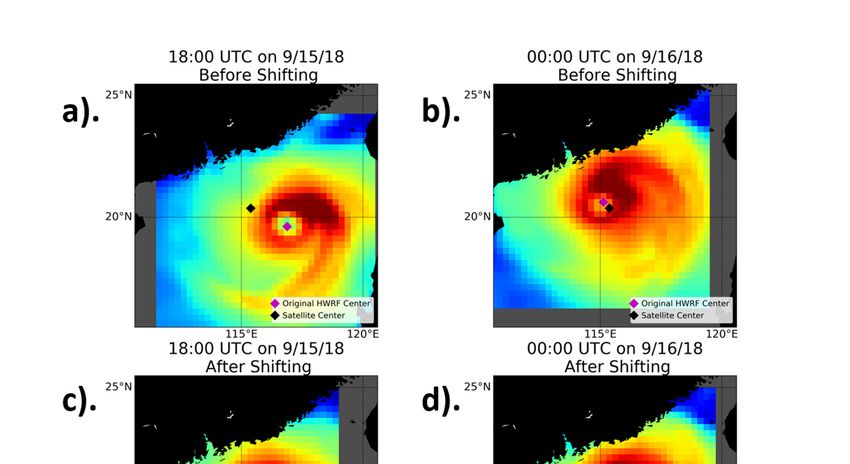
2. Data Sets
                                  2.1. SMAP Winds
Remote Sens. 2021, 13, 2347                                                                                                                   3 of 19
                                         Since 2017, RSS has been producing SMAP wind data in the form of twice-daily grid-
                                  ded maps (for ascending and descending swaths) on a 0.25 × 0.25 degree Earth grid. The
                                  original spatial resolution of the SMAP data is 40 km. These SMAP wind data are pro-
                                 grid.
                                  duced  Theinoriginal
                                                 near-realspatial
                                                                timeresolution
                                                                       (latency ofofthe  ~3SMAP
                                                                                              h) anddataare
                                                                                                          is 40   km. These
                                                                                                               freely           SMAP
                                                                                                                        available      to wind   data
                                                                                                                                           download
                                 are  produced in near-real time (latency ofaccessed
                                  (http://remss.com/missions/smap/winds/;                    ~3 h) and    areMay
                                                                                                      on 10     freely  available to download
                                                                                                                     2021).
                                 (http://remss.com/missions/smap/winds/; accessed on 10 May 2021).
                                  2.2. AMSR2 and WindSat TC-Winds
                                 2.2. AMSR2 and WindSat TC-Winds
                                         The TC-winds products are the result of a new algorithm that allows sensors with C-
                                  and The     TC-winds
                                        X- band     channelsproducts    are the
                                                                 to retrieve      resultinoftropical
                                                                               winds          a new algorithm
                                                                                                      cyclones, eventhat allows     sensors with
                                                                                                                           in the presence          C-
                                                                                                                                                of rain
                                 and   X-  band   channels     to retrieve   winds   in  tropical  cyclones,    even
                                  [4]. As with SMAP, the TC-winds from AMSR2 and WindSat consist of winds in tropical in the   presence   of  rain [4].
                                 As with SMAP, the TC-winds from AMSR2 and WindSat consist of winds in tropical
                                  cyclones in the form of daily gridded 0.25 × 0.25 degree maps for both ascending and
                                 cyclones in the form of daily gridded 0.25 × 0.25 degree maps for both ascending and
                                  descending           satellite      passes       and        are     freely       available        to     download
                                 descending satellite passes and are freely available to download (http://www.remss.com/
                                  (http://www.remss.com/tropical-cyclones/tc-winds/; accessed on 10 May 2021). The
                                 tropical-cyclones/tc-winds/; accessed on 10 May 2021). The AMSR2 data extend from
                                  AMSR2 data extend from 2012 to the present day, while the WindSat data extend from
                                 2012 to the present day, while the WindSat data extend from 2003 to October 2020, when
                                  2003 to October 2020, when WindSat ceased operation. The spatial resolution of the
                                 WindSat ceased operation. The spatial resolution of the AMSR2 and WindSat TC-winds
                                  AMSR2 and WindSat TC-winds is about 50 km, which is close to the spatial resolution of
                                 is about 50 km, which is close to the spatial resolution of the SMAP winds. Along with
                                  the SMAP winds. Along with wind speed, the WindSat TC-winds files contain values for
                                 wind speed, the WindSat TC-winds files contain values for wind direction, rain rate, and
                                  wind direction, rain rate, and ancillary sea surface temperature (SST). Similarly, the
                                 ancillary sea surface temperature (SST). Similarly, the AMSR2 TC-winds files contain rain
                                  AMSR2 TC-winds files contain rain rate and ancillary SST, as well as columnar water va-
                                 rate and ancillary SST, as well as columnar water vapor. It should be noted that, since the
                                  por. It should be noted that, since the AMSR2 and WindSat algorithms are specifically
                                 AMSR2 and WindSat algorithms are specifically trained in tropical cyclone conditions, they
                                  trained
                                 may         in tropical
                                       be less   accuratecyclone
                                                             in areasconditions,
                                                                        where SST they< 25 ◦may
                                                                                              C and bewind
                                                                                                       less accurate
                                                                                                              speed is in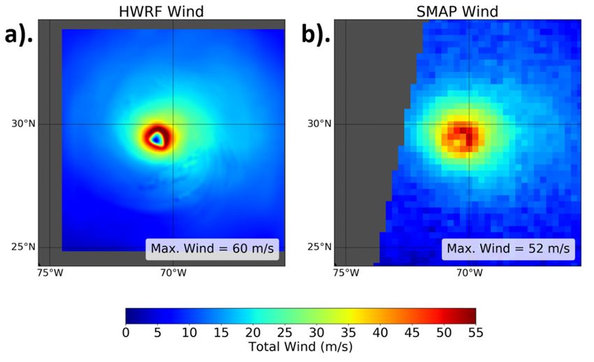
Remote Sens. 2021, 13, 2347                                                                                           4 of 19

                              (https://www.emc.ncep.noaa.gov/gc_wmb/vxt/HWRF/; https://ftpprd.ncep.noaa.gov/
                              data/nccf/com/hur/prod/; accessed on 10 May 2021) [25]). There are a large number
                              of HWRF model realizations of TC surface winds available from the past several years
                              that can be used for the TC-wind comparison. Since the HWRF model is operational and
                              does not have a publicly accessible data archive, these data were provided by request from
                              both the NOAA Environmental Modeling Center (EMC) and the University of Michigan
                              (David Mayers; personal communication). For our study, we obtained HWRF winds for 0-h
                              analyses at 00Z, 06Z, 12Z, and 18Z for 19 storms between 2017 and 2020 (see Appendix A for
                              information on how to download similar real-time data), and used them in a comparison
                              with the TC-winds satellite observations. Note that these 0-h analyses, which are produced
                              every 6 h, are not forecasts themselves, but rather initializations of the HWRF model. Each
                              0-h analysis contains a constructed vortex that is initialized using data assimilated from the
                              National Center for Environmental Prediction (NCEP) Global Data Assimilation System
                              (GDAS) 6-h forecasts, as well as conventional in situ observations, satellite observations,
                              and Doppler radar radial velocities where available [25]. We chose to use the HWRF 0-h
                              analyses as opposed to the HWRF forecasts (which are produced every 3 h starting at each
                              0-h analysis time) because the 0-h analyses are less dependent on the HWRF simulation
                              of storm motion/features. Thus, they can be expected to be more representative of the
                              structure and intensity of a tropical cyclone at a given analysis time.
                                   Additionally, the HWRF model contains three different gridded domains: one large
                              parent domain, and two nested inner domains. All three domains encompass the location
                              of the storm at each analysis time, with each subsequent nested domain from the parent
                              domain downward becoming successively smaller in area. In our study, we used data from
                              innermost domain and part of the surrounding domain. These data extended 9 × 9 degrees
                              and had a spatial resolution of approximately 1.5 km. The use of this fine-scale domain
                              allowed us to experiment with various methods of spatial resampling in order to find
                              the one that best captured the storms’ features as observed by the satellite and avoided
                              smoothing them out too much. An in-depth discussion of this spatial resampling is
                              presented in the following section.

                              3. Methods
                              3.1. Spatial Resampling
                                   One of the first and most important issues to address when comparing the satellite
                              TC-winds to those of a high-resolution model such as HWRF is the differences in spatial
                              scales between the two. The TC-winds measurements all have an approximate resolution
                              of 40–50 km and are reported on a 0.25 × 0.25 degree (≈25 km) Earth grid. This is much
                              coarser than the native resolution of the HWRF model used in this study. These differences
                              in spatial scales can lead to large differences between wind intensities and the features that
                              are resolved in the HWRF and satellite observations of the same storm. This is illustrated
                              in Figure 2, which shows a side-by-side comparison of HWRF and SMAP TC-winds for
                              Hurricane Florence on 12 September 2018 at 12:00 UTC and 10:50 UTC, respectively. It is
                              apparent that, despite the images being within about an hour of one another, the features
                              seen in the 2D wind fields at the two resolutions are quite different. For instance, the
                              HWRF wind field shows the eye of the hurricane to have wind speeds near zero, while the
                              SMAP observations show the eye winds to be closer to 35 m/s. It is also evident that the
                              maximum wind speeds seen in the HWRF model at its original resolution are larger than
                              the maximum wind speeds observed by the satellite.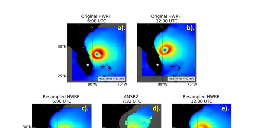
Remote Sens. 2021, 13, x FOR PEER REVIEW 5 of 20
Remote Sens. 2021, 13, 2347 5 of 19
evident that the maximum wind speeds seen in the HWRF model at its original resolution
are larger than the maximum wind speeds observed by the satellite.
Figure
Figure 2.2. Wind fields
fields of
of Hurricane
Hurricane Florence
Florence on
on 12
12 September
September 2018
2018 from
from the
the HWRF
HWRF model
model at at its
its
original
original resolution
resolution of of ~1.5
~1.5 km
km at
at 12:00
12:00 UTC
UTC (a)
(a) and
and from
from SMAP
SMAP TC-winds
TC-winds at at their
theirnative
nativeresolution
resolution
of 40
of 40 km
km atat 10:50
10:50 UTC
UTC (b).
(b). The
The maximum
maximum wind
wind value
value for
for each
each field
field at
at these
these resolutions
resolutionsisisshown
shownin in
the bottom
the bottom right
right of
of each
each panel.
panel.
In order
In order toto account
account for
for the
the differences
differences in inspatial
spatial scales,
scales, the
theHWRF
HWRF winds winds need
need totobe
be
resampled
resampledto tothe
the spatial
spatialresolution
resolutionof ofthe
thesatellite
satelliteobservations.
observations.This Thisisis done
doneby by calculating
calculating
the
the weighted
weighted average
average ofof the
the HWRF
HWRF wind wind field
field at
ateach
eachsatellite
satellitegrid
gridcell.
cell. The
The weight
weight isis
defined
defined by by the
the gain
gain pattern
pattern ofof the
the satellite
satellite antenna
antenna projected
projected ontoonto the
the Earth’s
Earth’s surface.
surface. WeWe
employed a frequently used gain pattern approximation that takes
employed a frequently used gain pattern approximation that takes the form of a radially the form of a radially
symmetric
symmetric Gaussian
Gaussian weighting
weighting function ( )
functionWW(r ) r(Figure 3): 3):
(Figure
W (r ) = exp − ln 2 · (r/r0 )2 2
(1)
W ( r ) = exp − ln 2 ⋅ r (1)
theHWRF
r0 wind measurement and the
In (1), r denotes the distance (in km) between
center of the 0.25 degree satellite product grid cell and r0 = D/2, where D is the geometric
In (1),
average r denotes
of the the distance
half-power footprint (indiameters.
km) between Thethe HWRF
values of Dwind measurement and
are approximately the
40 km
for SMAP,
center 48 km
of the 0.25for AMSR2
degree and 52
satellite km WindSat.
product grid cellThis r0 = D function
andweighting , where (1) D provides
is the geo-a
2
good approximation for the antenna gain over the main lobe and the near-side lobes of the
metric average of the half-power footprint diameters. The values of D are approxi-
antenna, and is sufficient for our purpose of approximately matching the spatial scales of
mately winds
HWRF 40 km to forthose
SMAP,
seen48bykmthe forsatellite.
AMSR2 and 52 km WindSat. This weighting function
(1) provides
Figure 4b shows the results offor
a good approximation thethe antenna gain
resampled HWRF overwind
the main
field lobe and thetonear-
compared the
side lobes of the antenna, and is sufficient for our purpose
SMAP wind field (Figure 4a). We see that this resampling method resulted of approximately matching
in a windthe
spatial scales of HWRF winds to those seen by the satellite.
field that captured the features seen in the satellite winds, and thus resembled the satellite
observation well.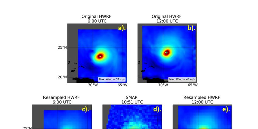
Remote Sens. 2021, 13, 2347                                                                                                              6 of 19
    Remote Sens. 2021, 13, x FOR PEER REVIEW                                                                                   6 of 20

 Remote Sens. 2021, 13, x FOR PEER REVIEW                                                                                                  7 of 20
                                   Figure 3.
                                   Figure 3.AAgraphical
                                                graphicalillustration of of
                                                           illustration  thethe
                                                                             Gaussian weighting
                                                                                Gaussian        method
                                                                                         weighting     applied
                                                                                                   method       to each
                                                                                                            applied     0.25 ×0.25
                                                                                                                     to each   0.25× 0.25 degree
                                   degree grid point as described in Equation (1). The half-power footprint diameter was 40 km.
                                     grid point as described in Equation (1). The half-power footprint diameter was 40 km.
                                           Figure 4b shows the results of the resampled HWRF wind field compared to the
                                     SMAP wind field (Figure 4a). We see that this resampling method resulted in a wind field
                                     that captured the features seen in the satellite winds, and thus resembled the satellite ob-
                                     servation well.
                                           For comparison, we also tested two other simple resampling schemes. Figure 4c
                                     shows the result for a ‘drop-in-the-bucket’ average for a 0.25 degree (~25 km) grid cell.
                                     This was calculated by averaging all HWRF observations within a given 0.25 degree grid
                                     cell and assigning the resulting wind speed to that grid cell. In other words, the weighting
                                     function W was set equal to 1 if the HWRF wind lies within the 0.25 degree grid cell,
                                     and 0 if it lay outside. The resulting resampled HWRF wind field resembled the Gaussian
                                     average reasonably well. It is feasible to use this averaging method for doing a quick and
                                     simple resampling. Figure 4d shows the resulting wind field when a drop-in-the-bucket
                                     average was performed within a 40 km box. The resampled HWRF wind field appeared
                                     much coarser, and features of the storm were more difficult to resolve when compared to
                                     both SMAP and the Gaussian average. A 40 km drop-in-the-bucket average should not be
                                     used when matching the spatial scales of the high-resolution HWRF field with the low-
                                     resolution satellite field. The physical reason for this is that, even if the actual satellite
                                     footprint is 40 km, the signal is not collected uniformly over that footprint diameter, but
                                     rather with a Gaussian-shaped gain, as illustrated above.

       Figure4.4.Various
      Figure      Various    methods
                          methods   of of resampling
                                       resampling  thethe HWRF
                                                       HWRF      data
                                                              data    from
                                                                   from     its native
                                                                        its native     resolution
                                                                                   resolution for afor a sample
                                                                                                    sample  viewview  of Hurricane
                                                                                                                 of Hurricane        Flor-
                                                                                                                                Florence
       ence  on  12 September    2018  at 12:00 UTC. (a) The SMAP  pass over  Hurricane   Florence  approximately  1 h before
      on 12 September 2018 at 12:00 UTC. (a) The SMAP pass over Hurricane Florence approximately 1 h before the HWRF time      the HWRF
       time shown
      shown   in (b–d),in(b)
                          (b–d),
                             HWRF (b)resampled
                                      HWRF resampled      using a weighting
                                                 using a Gaussian Gaussian weighting
                                                                              method withmethod
                                                                                            a 40 kmwith  a 40 kmwidth,
                                                                                                     half-power   half-power    width, (c)
                                                                                                                         (c) resampling
       resampling using a 25 km drop-in-the-bucket box average, and (d) resampling using a 40 km drop-in-the-bucket box av-
      using a 25 km drop-in-the-bucket box average, and (d) resampling using a 40 km drop-in-the-bucket box average.
       erage.

                                          Figure 5 shows an example of the Gaussian weighting method applied to the HWRF
                                      winds at times surrounding a SMAP pass for the case of Hurricane Dorian on 30 August
                                      2019. The top two panels display the HWRF wind fields at the original HWRF resolution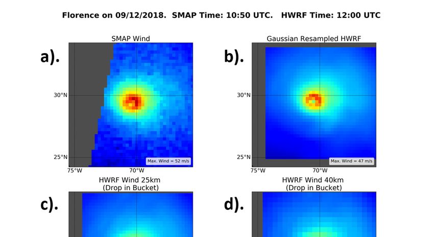
Remote Sens. 2021, 13, 2347                                                                                                          7 of 19

                                           For comparison, we also tested two other simple resampling schemes. Figure 4c shows
                                      the result for a ‘drop-in-the-bucket’ average for a 0.25 degree (~25 km) grid cell. This was
                                      calculated by averaging all HWRF observations within a given 0.25 degree grid cell and
                                      assigning the resulting wind speed to that grid cell. In other words, the weighting function
                                      W was set equal to 1 if the HWRF wind lies within the 0.25 degree grid cell, and 0 if it
                                      lay outside. The resulting resampled HWRF wind field resembled the Gaussian average
                                      reasonably well. It is feasible to use this averaging method for doing a quick and simple
                                      resampling. Figure 4d shows the resulting wind field when a drop-in-the-bucket average
                                      was performed within a 40 km box. The resampled HWRF wind field appeared much
                                      coarser, and features of the storm were more difficult to resolve when compared to both
                                      SMAP and the Gaussian average. A 40 km drop-in-the-bucket average should not be used
                                      when matching the spatial scales of the high-resolution HWRF field with the low-resolution
                                      satellite field. The physical reason for this is that, even if the actual satellite footprint is
                                      40 km, the signal is not collected uniformly over that footprint diameter, but rather with a
                                      Gaussian-shaped gain, as illustrated above.
                                           Figure 5 shows an example of the Gaussian weighting method applied to the HWRF
                                      winds at times surrounding a SMAP pass for the case of Hurricane Dorian on 30 August
                                      2019. The top two panels display the HWRF wind fields at the original HWRF resolution
                                      both before and after the SMAP pass. The bottom left (Figure 5c) and bottom right panels
                                      (Figure 5e) show the same HWRF wind fields that have been resampled to the satellite res-
                                      olution using the Gaussian weighting method, while the bottom middle panel (Figure 5d)
                                      shows the winds from the SMAP pass itself. It can be seen by comparing the resampled
                                      HWRF wind fields to that of SMAP that the chosen Gaussian resampling method resulted
                                      inREVIEW
      Remote Sens. 2021, 13, x FOR PEER  model winds that closely resembled both the structure and intensity seen by the8 satellite.
                                                                                                                              of 20
                                      For example, in Figure 5, both the resampled HWRF wind fields, as well as SMAP, show a
                                      distinct band of winds in the SE quadrant of similar intensity and shape, despite the wind
                                      fields being several hours apart.

           Figure
      Figure      5. Comparison
             5. Comparison       of SMAP
                             of SMAP  andand HWRF
                                          HWRF      winds
                                                   winds   forHurricane
                                                         for   HurricaneDorian
                                                                        Dorian on 30 August
                                                                                      August2019
                                                                                               2019for
                                                                                                    fora aSMAP
                                                                                                           SMAP  pass at 10:51
                                                                                                                   pass        UTC.
                                                                                                                         at 10:51 UTC.
           Top  panels: the HWRF  winds before resampling for the HWRF  analysis times before (a) and  after (b) the corresponding
      Top panels: the HWRF winds before resampling for the HWRF analysis times before (a) and after (b) the corresponding
           SMAP pass. Bottom panels: the resampled HWRF winds at analysis times before (c) and after (e) the SMAP pass (d).
      SMAP pass. Bottom panels: the resampled HWRF winds at analysis times before (c) and after (e) the SMAP pass (d).

                                            Another example of an application of the resampling method using Gaussian
                                      weighting is seen in Figure 6, which presents the wind fields in the same manner as Figure
                                      5 for an AMSR2 pass over Hurricane Dorian on 4 September 2019 at 7:32 UTC. The AMSR2
                                      pass did not observe Dorian’s winds right near the coast, as they were flagged for con-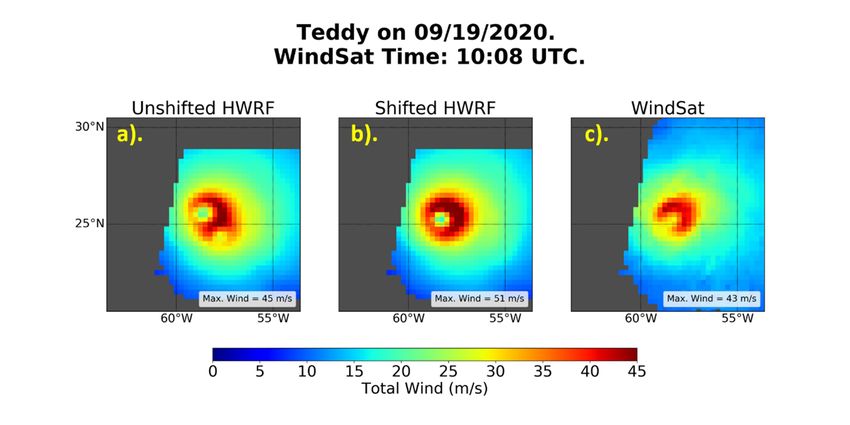
Remote Sens. 2021, 13, 2347 8 of 19
Another example of an application of the resampling method using Gaussian weight-
ing is seen in Figure 6, which presents the wind fields in the same manner as Figure 5 for
an AMSR2 pass over Hurricane Dorian on 4 September 2019 at 7:32 UTC. The AMSR2 pass
did not observe Dorian’s winds right near the coast, as they were flagged for contamination
from land emission. The similarities between the satellite and the resampled HWRF wind
fields are evident. The size of the eye, as well as the magnitude of the winds within it, in the
resampled HWRF closely resemble those seen by AMSR2. The same applies for the band
of strong winds in the NE quadrant of the eyewall. The agreement between AMSR2 and
Remote Sens. 2021, 13, x FOR PEERthe resampled HWRF was best for the HWRF wind field at 6:00 UTC, which was9 closest
REVIEW of 20
to the AMSR2 overpass. Consistent storm structures and intensities were seen between
the models and satellite sensors for most of the 19 storms analyzed in this study. These 19
storms are listed in Table 1.
Figure
Figure 6. Comparison
6. Comparison of AMSR2
of AMSR2 and
and HWRFwinds
HWRF windsforforHurricane
HurricaneDorian
Dorian on 4 September
September2019
2019for
forananAMSR2
AMSR2pass passatat 7:32
7:32
UTC. TopUTC. Topthe
panels: panels:
HWRF thewinds
HWRFbefore
windsresampling
before resampling for the analysis
for the HWRF HWRF analysis times(a)
times before before
and (a) and
after (b)after (b) the cor-
the corresponding
responding SMAP pass. Bottom panels: the resampled HWRF winds at analysis times before (c) and after (e) the AMSR2
SMAP pass. Bottom panels: the resampled HWRF winds at analysis times before (c) and after (e) the AMSR2 pass (d).
pass (d).
Table 1. The 19 storms analyzed in this study, along with the dates during their lifetimes for which
Table 1. The 19 storms analyzed in this study, along with the dates during their lifetimes for which
available satellite overpasses were compared to HWRF data. A full list of satellite passes over each of
available satellite overpasses were compared to HWRF data. A full list of satellite passes over each
these storms
of these is provided
storms in the
is provided Supplementary
in the Materials.
Supplementary Materials.
Storm
Storm Basin
Basin Dates
Dates
Harvey
Harvey Atlantic
Atlantic 18
18 August 2017–30August
August 2017–30 August2017
2017
Irma
Irma Atlantic
Atlantic 11 September 2017–12September
September 2017–12 September2017
2017
JoseJose Atlantic
Atlantic 15 September
15 September 2017–22
2017–22September
September2017
2017
Maria
Maria Atlantic
Atlantic 17 September 2017–30 September 2017
17 September 2017–30 September 2017
18 August 2018; 20 August 2018; 23 August 2018–24
Lane Pacific 18 August 2018; 20 August 2018; 23 August 2018–
Lane Pacific August 2018
Jebi Pacific 28 August242018–4
August 2018
September 2018
Jebi
Florence Pacific
Atlantic 1 28 August 2018–4
September 2018–16September
September 2018
2018
Mangkhut
Florence Pacific
Atlantic 17 September
September 2018–16
2018–16September
September2018
2018
Mangkhut Pacific 7 September 2018–16 September 2018
Trami Pacific 23 September 2018–24 September 2018
Michael Atlantic 7 October 2018–12 October 2018
Yutu Pacific 23 October 2018; 26 October 2018–27 October 2018
9 March 2019–10 March 2019; 12 March 2019–14
Idai Southern Hemisphere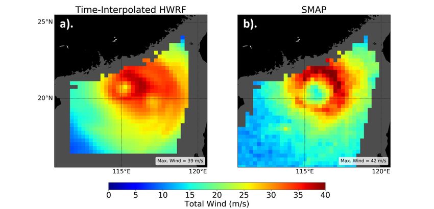
Remote Sens. 2021, 13, 2347 9 of 19
Table 1. Cont.
Storm Basin Dates
Trami Pacific 23 September 2018–24 September 2018
Michael Atlantic 7 October 2018–12 October 2018
Yutu Pacific 23 October 2018; 26 October 2018–27 October 2018
9 March 2019–10 March 2019; 12 March 2019–14
Idai Southern Hemisphere
March 2019
Dorian Atlantic 25 August 2019–7 September 2019
26 September 2019–27 September 2019; 29 September
Remote Sens. 2021, 13, x FOR PEERLorenzo
REVIEW Atlantic
2019–1 October 2019; 9 October 201910 of 20
Hagibis Pacific 6 October 2019–13 October 2019
Laura Atlantic 21 August 2020–27 August 2020
Haishen Pacific 1 September 2020–7 September 2020
Laura Atlantic 21 August 2020–27 August 2020
Paulette Atlantic 7 September 2020–23 September 2020
Haishen Pacific 1 September 2020–7 September 2020
Teddy Atlantic 14 September 2020–23 September 2020
Paulette Atlantic 7 September 2020–23 September 2020
Teddy Atlantic 14 September 2020–23 September 2020
3.2. Time Interpolation
3.2.
InTime
this Interpolation
section, we address the temporal mismatch between HWRF and the satellite
observations. In order
In this section, wetoaddress
facilitate
the atemporal
more direct
mismatchcomparison between
between HWRF andthethesatellites
satellite and
the observations.
models, the spatially
In order toresampled HWRF
facilitate a more wind
direct fields from
comparison the model
between times surrounding
the satellites and the
eachmodels,
satellitethepass
spatially
wereresampled
interpolatedHWRF wind
to the fields
time fromsatellite
of the the model windtimes surrounding
field. The resulting
each satellite pass
time-interpolated 2Dwere
HWRFinterpolated
wind fieldsto thecould
time of
bethe satellite wind
compared to thefield. The resulting
satellite observations.
time-interpolated
However, this simple 2Dtime
HWRF wind fields could
interpolation may be notcompared
properlytoaccount
the satellite
for observations.
the movement of
the However, this simple time interpolation may not properly account for the movement of
storm in space and time, which in some cases could result in spurious and unrealistic
the storm in space and time, which in some cases could result in spurious and unrealistic
features in the time-interpolated fields.
features in the time-interpolated fields.
AnAn example of this is provided in Figure 7, which shows the resampled HWRF wind
example of this is provided in Figure 7, which shows the resampled HWRF wind
field
field that has beeninterpolated
that has been interpolated to the time
to the timeofofa aSMAP
SMAP overpass
overpass overover Typhoon
Typhoon Mangkhut
Mangkhut
on 15
on 15 September 2018 at 22:34 UTC. An un-physical double-eye feature is clearly seen in seen
September 2018 at 22:34 UTC. An un-physical double-eye feature is clearly
in the
the time-interpolated
time-interpolated HWRF HWRF windwind field.
field. Spurious
Spurious features
features like
like this canthis can when
emerge emerge thewhen
the wind
windfieldfieldofofwell-organized
well-organized and/or rapidly changing/moving storms
and/or rapidly changing/moving storms is interpolated be- is interpolated
between
tween two 6-h scenes.
two 6-h scenes.Care
Care must
must be be taken
taken when when comparing
comparing satellite
satellite and HWRFand HWRF
winds inwinds
these instances.
in these instances.
FigureFigure
7. The7.resampled
The resampled
HWRF HWRF
windwind
fieldfield
thatthat
has has
beenbeen interpolated
interpolated (a)(a)
to to
thethe timeofofthe
time theSMAP
SMAPpasspass (22:34
(22:34 UTC)
UTC) (b)
(b) over
over Typhoon Mangkhut on 15 September 2018. An un-physical double-eye feature is clearly visible in the resampled
Typhoon Mangkhut
HWRF field. on 15 September 2018. An un-physical double-eye feature is clearly visible in the resampled HWRF
field.
In order to address these types of cases, an intermediate step can be taken between
In order to
resampling of address these types
the high-resolution of cases,
data an intermediate
and performing step interpolation.
the temporal can be takenThis
between
resampling
involves spatially shifting the two resampled wind fields surrounding a given satellite This
of the high-resolution data and performing the temporal interpolation.
pass so that their storm centers align with the storm center as seen by the satellite; i.e.,
shifting the model winds into a storm-centric coordinate system [26,27]. To perform this
shifting, the storm center as seen by the satellite was first visually determined from a plot
of the observed wind field with the aid of the Best Track data of the National Hurricane
Center (NHC) [28]. Next, the storm centers from the resampled HWRF fields surrounding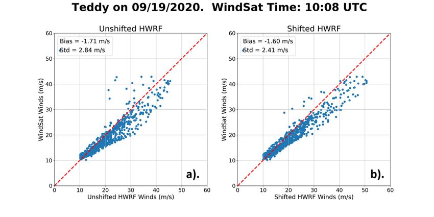
Remote Sens. 2021, 13, 2347 10 of 19
involves spatially shifting the two resampled wind fields surrounding a given satellite pass
so that
Remote Sens. 2021, 13, x FOR PEER their
REVIEW storm centers align with the storm center as seen by the satellite; i.e., 11 shifting
of 20
the model winds into a storm-centric coordinate system [26,27]. To perform this shifting,
the storm center as seen by the satellite was first visually determined from a plot of the
observed
over wind
Typhoon field with theon
Mangkhut aid
15of the Best 2018.
September TrackThe data
topoftwo
thepanels
National showHurricane
the resampledCenter
(NHC) [28]. winds
HWRF Next, surrounding
the storm centersthe SMAP from passthebefore
resampled HWRF
shifting, and the fields surrounding
bottom two panelsthe
show
satellite passthewere
samevisually
resampled HWRF winds
determined shiftedOnce
as well. to thethis
SMAP wascenter.
done,The both satellite center 2D
resampled
and the original HWRF centers are marked by the black
HWRF wind fields were fully shifted so that the HWRF storm centers aligned with theand magenta diamonds, respec-
tively.
satellite stormIt can be seen
center. Thisin process
the figureisthat the HWRF
illustrated storm centers
in Figure 8 for the(i.e.,case
the eyes)
of thewere
SMAP coin-pass
cident with the magenta diamond (the initial HWRF storm
over Typhoon Mangkhut on 15 September 2018. The top two panels show the resampled centers) in Figure 8a,b (the
HWRF wind fields before shifting was performed). In Figure 8c,d, the resampled HWRF
HWRF winds surrounding the SMAP pass before shifting, and the bottom two panels show
2D wind fields have been shifted so that their storm centers were coincident with the lo-
the same resampled HWRF winds shifted to the SMAP center. The satellite center and
cation of the satellite storm center (the black diamond). Once this shifting was performed,
the original
the HWRF HWRF datacenters
could beare marked by
interpolated the time
to the blackofand magenta
the satellite diamonds,
overpass. This respectively.
was done
It canbybetaking
seen in the figure
a weighted that the
average HWRF
of the storm centers
two resampled HWRF (i.e.,
windthefields
eyes) were coincident
surrounding the
with the magenta
satellite diamond
observation, with(the
moreinitial
weight HWRFapplied storm
to thecenters)
HWRF winds in Figurethat 8a,b
were(the
closerHWRF
in
wind time
fieldstobefore shifting
the overpass. was
The performed).
steps of this shifting In Figure 8c,d, the
methodology canresampled
be summarized HWRF 2D wind
as follows
fields and
havecanbeen shiftedto
be applied soany
thathigh-resolution
their storm centers data set,were
suchcoincident
as HWRF, with whenthe locationitof
comparing to the
satellite
satellite storm data in tropical
center storms:
(the black diamond). Once this shifting was performed, the HWRF
data could be interpolated
1. Resample to the time
the high-resolution dataof to
thethesatellite overpass.
same spatial Thisaswas
resolution the done by(Sec-
satellite taking
a weighted tionaverage
3.1). of the two resampled HWRF wind fields surrounding the satellite
2. Shift
observation, the resampled
with more weight storm windsto
applied at the
the model
HWRFtimes windssurrounding
that werethe satellite
closer passto
in time sothe
that their storm centers align with the storm center as seen
overpass. The steps of this shifting methodology can be summarized as follows and can be by the satellite.
applied3. toLinearly interpolate thedata
any high-resolution modelset,wind
suchfield to the same
as HWRF, when time as the satellite
comparing it to pass.
satellite data
in tropical storms:
Figure 8. Figure 8. Top panels:
Top panels: The resampled
The resampled HWRF HWRF
windswinds at model
at model times
times before(a)
before (a)and
andafter
after (b)
(b) the
the SMAP
SMAPpass
passover Typhoon
over Typhoon
Mangkhut on 15 September 2018 at 22:34 UTC before spatial shifting was performed. Bottom panels: The resampled
Mangkhut on 15 September 2018 at 22:34 UTC before spatial shifting was performed. Bottom panels: The resampled
HWRF winds at model times before (c) and after (d) the SMAP pass after spatial shifting was performed. The SMAP storm
HWRF
winds at model
center istimes before
indicated by(c)
theand after
black (d) theThe
diamond. SMAP passHWRF
original after spatial shifting
storm center was performed.
is indicated The SMAP
by the magenta storm center is
diamond.
indicated by the black diamond. The original HWRF storm center is indicated by the magenta diamond.Remote Sens. 2021, 13, 2347 11 of 19
Resample the high-resolution data to the same spatial resolution as the satellite
(Section 3.1).
Remote Sens. 2021, 13, x FOR PEER REVIEWShift the resampled storm winds at the model times surrounding the satellite pass 12 ofso20
that their storm centers align with the storm center as seen by the satellite.
Linearly interpolate the model wind field to the same time as the satellite pass.
The
Theresult
resultofofusing
usingthis
thismethodology
methodologyon onthetheHWRF
HWRFwindswindssurrounding
surroundingthe theSMAPSMAP
pass
passofofTyphoon
Typhoon Mangkhut
Mangkhut on 15 September
September 2018 2018isisshown
shownininFigure
Figure9.9.It is
It clear
is clearthatthat
the
the resulting
resulting HWRF
HWRF windwind field
field is more
is more realistic
realistic thanthan
thethe
oneone obtained
obtained fromfrom interpolating
interpolating un-
un-shifted
shifted windswinds (Figure
(Figure 7a), the
7a), and anddouble-eye
the double-eyefeaturefeature is no present.
is no longer longer present. It also
It also compares
compares better to the SMAP winds for this pass (Figure 7b). For instance,
better to the SMAP winds for this pass (Figure 7b). For instance, the location of the maxi- the location
of the maximum
mum winds in the winds in the NE in
NE quadrant quadrant
Figure 9inisFigure
more in9 isline
more in their
with line with theiraslocation
location seen by
as seen by the satellite. We also noted that the value for the maximum
the satellite. We also noted that the value for the maximum intensity (43 m/s) agreed intensity (43 m/s)
better
agreed
with thebetter
SMAP with the SMAP
intensity (42 intensity
m/s) than(42 m/s)
if no than
shift wasif performed
no shift was performed
(39 m/s). There (39arem/s).
still
There are still differences between the resampled and shifted HWRF
differences between the resampled and shifted HWRF field and SMAP, but the compari- field and SMAP, but
the
soncomparison is clearly
is clearly better than better
without than without
aligning thealigning the storm centers.
storm centers.
Figure9.9. The
Figure The resampled
resampled HWRF
HWRF wind
wind field
field to
tobe
becompared
comparedwith
withthe
theSMAP
SMAPpass
passover
overTyphoon
Typhoon
Mangkhut on 15 September 2018 created by first shifting the surrounding HWRF winds before in-
Mangkhut on 15 September 2018 created by first shifting the surrounding HWRF winds before
terpolating.
interpolating.
Anotherexample
Another exampleofofthis
thisshifting
shiftingmethodology
methodologyisisshown
shownin inFigure
Figure10 10for
foraaWindSat
WindSat
pass over Hurricane Teddy on 19 September 2020. It can be seen that shifting
pass over Hurricane Teddy on 19 September 2020. It can be seen that shifting the surround- the sur-
rounding
ing HWRFHWRF wind first
wind fields fields(Figure
first (Figure 10b) removed
10b) removed the double-eye
the double-eye feature
feature present
present in thein
the original interpolation method (Figure 10a). The storm structure when the
original interpolation method (Figure 10a). The storm structure when the shifting was usedshifting was
used corresponded much better with the WindSat field than in the unshifted
corresponded much better with the WindSat field than in the unshifted case. For example, case. For
example, the locations of the eye and the relative maxima of winds in the eye
the locations of the eye and the relative maxima of winds in the eye wall in the NW, NE, wall in the
NW, NE, and SE quadrants in the shifted wind field are now in approximately the same
location as they were in the satellite wind field.Remote Sens. 2021, 13, 2347 12 of 19
Remote Sens. 2021, 13, x FOR PEER REVIEW 13 of 20
and SE quadrants in the shifted wind field are now in approximately the same location as
they were in the satellite wind field.
Figure 10. Three wind fields for the WindSat pass over Hurricane Teddy on 19 September 2020 at 10:08 UTC. (a) The
Figure 10. HWRF
resampled Three wind
wind fields for has
field that the been
WindSat pass over
temporally HurricanetoTeddy
interpolated onof19the
the time September 2020 at 10:08
WindSat overpass, UTC.
(b) the (a) The
resampled
resampled HWRF wind field that has been temporally interpolated to the time of the WindSat overpass, (b) the
HWRF winds that have been shifted to the WindSat storm center and then temporally interpolated to the time of the resampled
HWRF winds that have been shifted to the WindSat storm center and then temporally interpolated to the time of the
WindSat overpass; i.e., the shifting methodology described in the text, and (c) the wind field from the WindSat pass itself.
WindSat overpass; i.e., the shifting methodology described in the text, and (c) the wind field from the WindSat pass itself.
It should be noted that using this shifting methodology generally provides the most
It shouldin
improvement becases
noted that using
where a morethis shifting methodology
well-organized storm has generally
moved rapidly provides the most
between two
improvement in cases where a more well-organized storm has
analysis times. In other cases; i.e., if the storm is less organized and/or slower moving, moved rapidly between
two
or ifanalysis times. In otherbetween
one is interpolating cases; i.e., if the
two storm
times thatis less
are organized
closer thanand/or slower
6 h apart moving,
(e.g., 3 h),
or if one is interpolating between two times that are closer
the relative improvement provided by shifting the surrounding HWRF storm centers than 6 h apart (e.g., 3 h), the
to
relative
the satelliteimprovement
storm center provided
is smallbyorshifting the surrounding
negligible. The use of this HWRF storm centers
methodology alsotodoes
the
satellite
not generally stormhave center is small
a large oron
effect negligible. The use comparisons
overall statistical of this methodology also
of satellite and does not
model
generally
winds, have a large
particularly effect
in cases onmany
with overall statisticalFor
matchups. comparisons
example, Figure of satellite
11 showsandside-by-
model
winds, particularly
side scatterplots in cases with
comparing many matchups.
matchups between WindSat For example,
windsFigure
and both11 shows side-by-
the unshifted
side scatterplots
(Figure comparing
11a) and shifted matchups
(Figure between WindSat
11b) interpolated HWRF fields winds forand
the both the unshifted
WindSat pass over
(Figure 11a) and shifted (Figure 11b) interpolated HWRF fields
Hurricane Teddy shown in Figure 10. It can be seen that, in this case, shifting the for the WindSat pass over
HWRF
Hurricane Teddy shown in Figure 10. It can be seen that, in
winds prior to performing time interpolation led to a slight improvement in standard this case, shifting the HWRF
winds
deviation prior to performing
and time interpolation
very little change in the valueled ofto a slight
the overallimprovement in standardwith
bias when compared de-
viation and
WindSat for very
winds little change
between 10in the60
and value
m/s.ofWe thefound
overall bias
that thiswhen
held compared
for most ofwith Wind-
the storms
Sat
thatforwewindsused between 10 and
in our study. 60 m/s. We
Ultimately, onefound
needs that
to this
lookheld for most
at each of the storms
individual storm casethat
we
andusedjudgeinifour study.time
a simple Ultimately, one needs
interpolation to lookoratifeach
is sufficient, individual
the more storm case
cumbersome and
shifting
judge if a simple
methodology timetointerpolation
needs be applied. In is general,
sufficient, if or
oneif is
the more cumbersome
performing statisticalshifting meth-
comparisons
odology
involvingneeds manytostorms/passes,
be applied. In the general,
use ofif this
one shifting
is performing statistical
methodology cancomparisons
be expectedin- to
volving
have little manyto no storms/passes,
impact on thethe use ofresults.
overall this shifting methodology can be expected to have
little to no impact on the overall results.Remote Sens. 2021, 13, 2347 13 of 19
Remote Sens. 2021, 13, x FOR PEER REVIEW 14 of 20
Figure 11. Scatterplots of WindSat matchups with interpolated resampled HWRF fields for Hurricane Teddy on 19
Figure 11. 2020
September Scatterplots
at 10:08of WindSat
UTC. matchups
(a) shows withwith
matchups interpolated
the HWRFresampled
wind fieldHWRF fields
that has beenfortemporally
Hurricaneinterpolated
Teddy on 19toSep-
the
tember 2020 at 10:08 UTC. (a) shows matchups with the HWRF wind field that has been temporally interpolated
time of the WindSat overpass. (b) shows matchups with the HWRF wind field created by first shifting then interpolating to the
time of the WindSat overpass. (b) shows matchups with the HWRF wind field created by first shifting then interpolating
the surrounding winds. The dashed red line represents the one-to-one line (i.e., no bias).
the surrounding winds. The dashed red line represents the one-to-one line (i.e., no bias).
4.
4. Results
Results
This
This section
sectionconducts
conductsa detailed statistical
a detailed comparison
statistical between
comparison the satellite
between TC-winds
the satellite TC-
and
winds and modeled HWRF winds for 19 storms in various ocean basins betweenand
modeled HWRF winds for 19 storms in various ocean basins between 2017 20172020.
and
These comparisons were made after the HWRF winds were resampled to the same spatial
2020. These comparisons were made after the HWRF winds were resampled to the same
resolution as the satellites using the Gaussian weighting method detailed in Section 3.1
spatial resolution as the satellites using the Gaussian weighting method detailed in Sec-
and temporally interpolated to the same time as the satellite.
tion 3.1 and temporally interpolated to the same time as the satellite.
4.1. Overall Results
4.1. Overall Results
Figure 12 shows scatterplots of matchups between the TC-winds and resampled
Figure 12 shows scatterplots
and time-interpolated HWRF forofeach matchups between the
of the AMSR2, SMAP,TC-winds and resampled
and WindSat sensors and
for
time-interpolated HWRF for each of the AMSR2, SMAP, and WindSat
passes over 19 storms across all ocean basins between the years of 2017 and 2020. sensors forOverall,
passes
over 19
good storms across
agreement can beallseen
ocean basins between
between the years
the satellites and ofthe2017 and 2020.
resampled Overall,
HWRF good
wind in
agreement can be seen between the satellites and the resampled HWRF
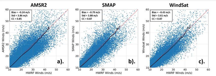
terms of bias (−0.24 m/s, −0.79 m/s, and −0.43 m/s for AMSR2, SMAP, and WindSat, wind in terms of
bias (−0.24 m/s, −0.79 m/s, and −0.43 m/s for AMSR2, SMAP, and WindSat,
respectively), standard deviations (3.86 m/s, 3.88 m/s, and 3.61 m/s for AMSR2, SMAP, respectively),
standard
and deviations
WindSat, (3.86 m/s,
respectively), 3.88
and m/s, and coefficient
correlation 3.61 m/s for AMSR2,
(0.85, 0.87, SMAP,
and 0.87and
forWindSat,
AMSR2,
respectively), and correlation coefficient (0.85, 0.87, and
SMAP, and WindSat, respectively) for winds between 10 m/s and 60 m/s.0.87 for AMSR2, SMAP, and
WindSat, respectively) for winds between 10 m/s and 60 m/s.
In Figure 13, we show the average satellite-HWRF bias and standard deviations, which
were binned vs. the average satellite/HWRF wind in 2 m/s wide bins between 10–30 m/s
and in 5 m/s wide bins from 30 m/s upward. This was done to ensure that the bins
were sufficiently populated. If there were less than 50 matchups in a given bin, it was not
included in this figure. The biases between the three sensors and HWRF were, in general,
relatively small, falling between ~0 m/s and −2.5 m/s for wind speeds between 10 and
40 m/s before becoming more positive at higher wind speeds. The standard deviations
tended to increase approximately linearly as wind speed increased, and leveled off slightly
at higher wind speeds. In general, the standard deviation for WindSat was slightly smaller
than for SMAP and AMSR2. Overall, Figure 13 indicates good consistency among the three
satellite sensors SMAP, AMSR2, and WindSat when all of them are compared to HWRF.
This is not too surprising, as the statistical TC wind algorithms for AMSR2 and WindSat
were trained with SMAP winds [4].time-interpolated HWRF for each of the AMSR2, SMAP, and WindSat sensors for passes
over 19 storms across all ocean basins between the years of 2017 and 2020. Overall, good
agreement can be seen between the satellites and the resampled HWRF wind in terms of
bias (−0.24 m/s, −0.79 m/s, and −0.43 m/s for AMSR2, SMAP, and WindSat, respectively),
Remote Sens. 2021, 13, 2347 standard deviations (3.86 m/s, 3.88 m/s, and 3.61 m/s for AMSR2, SMAP, and WindSat,
14 of 19
respectively), and correlation coefficient (0.85, 0.87, and 0.87 for AMSR2, SMAP, and
WindSat, respectively) for winds between 10 m/s and 60 m/s.
Remote Sens. 2021, 13, x FOR PEER REVIEW 15 of 20
Figure 12. Scatterplots of AMSR-2 (a), SMAP (b), and WindSat (c) winds plotted against HWRF winds that have been
temporally interpolated to the time of satellite overpasses for all 19 storms between 2017 and 2020 analyzed in this study.
The bias, standard deviation, and correlation coefficient for all wind speed matchups >10 m/s and 1013
m/s and 30 m/s. This was done to ensure the bins were sufficiently populated. If
were used for average winds >30 m/s. This was done to ensure the bins were sufficiently populated. If there were less thanthere were less than
5050matchups
matchupsinina agiven
givenbin,
bin,ititwas
wasnot
notincluded
includedininthis
thisfigure.
figure.The
Theblack
blackdashed
dashedline
lineisisthe
thezero-bias
zero-biasline.
line.
4.2. Atlantic vs. Pacific
To further examine the overall differences between the TC-winds and HWRF, we
separated the storms in this study by ocean basin (Atlantic or Pacific) and compared the
differences. This separation resulted in 11 storms in the Atlantic and seven storms in the
Pacific (one storm was located in the Southern Ocean and was not included in either ofRemote Sens. 2021, 13, 2347 15 of 19
4.2. Atlantic vs. Pacific
To further examine the overall differences between the TC-winds and HWRF, we
Remote Sens. 2021, 13, x FOR PEER REVIEW 16 of 20
separated the storms in this study by ocean basin (Atlantic or Pacific) and compared the
differences. This separation resulted in 11 storms in the Atlantic and seven storms in the
Pacific (one storm was located in the Southern Ocean and was not included in either of
these plots)
these plots) between
between 2017 2017 and
and 2020.
2020. Similar
Similar to
to Figure
Figure 13,
13, Figure
Figure 14
14 shows
shows the
the wind
wind biases
biases
and standard deviations between
and between each
each of
ofthe
thesensors
sensorsandandHWRF
HWRFseparated
separatedby bybasin.
basin.It It
is
evident that the satellites and HWRF were in better agreement in the
is evident that the satellites and HWRF were in better agreement in the Atlantic OceanAtlantic Ocean than
the Pacific.
than In the
the Pacific. Atlantic,
In the thethe
Atlantic, bias between
bias between thethe
sensors
sensorsand
andHWRF
HWRFwas was near
near zero for
for
winds of
winds of up
up to to35–40
35–40m/s.
m/s. In contrast, the bias in the the Pacific
Pacific quickly
quickly became
became negative
negative as
as
wind
wind speed
speed increased,
increased, staying consistently between −2 −2and
and−5 −m/s
5 m/s from
from approximately
approximately 25
25
to to
45 45 m/s
m/s before
before switching
switching signsatathigher
signs higherwind
windspeeds,
speeds,while
while maintaining
maintaining roughly the the
same magnitude as the lower wind speed bias. The standard deviation
same magnitude as the lower wind speed bias. The standard deviation between satellites between satellites
and
and HWRF
HWRF winds
winds at at higher
higher winds
winds(above
(above30–35
30–35m/s)
m/s) also was significantly
significantly lower
lower in
in the
the
Atlantic.
Atlantic. We note note that
that although
although there werewere fewer
fewer storms
storms in the
the Pacific
Pacific than
than the
the Atlantic,
Atlantic,
and
and thus
thus also
also fewer
fewer matchups
matchups withwith the
the satellites,
satellites, the
the bin
bin populations
populations in in each
each case
case were
were
sufficiently
sufficiently large
large toto make
make aa meaningful
meaningfulcomparison.
comparison.
Figure 14. The
Figure 14. The results
resultsshown
shownininFigure
Figure13,
13,except separated
except separatedinto thethe
into Atlantic (a) (a)
Atlantic andand
Pacific (b) basins.
Pacific (b) ba-
sins. Data
Data from from 11 storms
11 storms were to
were used used to make
make the curves
the curves for thefor the Atlantic,
Atlantic, while while data 7from
data from 7 storms
storms were
were used to make curves for the
used to make curves for the Pacific. Pacific.
the algorithms
Since the algorithms for the the each
each ofof sensors
sensors diddid not
not change
change from
from basin
basin to to basin,
basin, itit
could be concluded
could be concluded that the
the differences seen between the basins were most likely due
differences seen between the basins were most likely due to
to
differences
differences in in the
the HWRF
HWRF model.model. As noted
noted inin [25],
[25], the
the HWRF
HWRF analysis
analysis times
times assimilate
assimilate
observational
observational data data such
such asas conventional
conventional observations,
observations, satellite
satellite observations,
observations, and and Doppler
Doppler
radar
radar radial
radial velocities
velocities whenever
whenever available.
available. Most
Most of of these
these assimilated
assimilated datadata are
are gathered
gathered inin
situ,
situ, and
andareareoften
oftenmuch
much easier to to
easier collect in the
collect Atlantic
in the Basin
Atlantic due to
Basin duemany tropical
to many cyclones’
tropical cy-
proximity to land. This
clones’ proximity is inThis
to land. contrast
is intocontrast
the Pacific Basin,
to the where
Pacific mostwhere
Basin, storms are too
most remote
storms are
to be observed using any method other than satellites. Therefore,
too remote to be observed using any method other than satellites. Therefore, the initial the initial HWRF 0-h
analysis
HWRF 0-h vortices in the
analysis Atlantic
vortices willAtlantic
in the often bewill
constrained by more assimilated
often be constrained by more in situ data
assimilated
than
in situthose
datainthan
the Pacific,
those inandtheare likely and
Pacific, to more
are closely
likely to resemble the storm’s
more closely resembleactualthestructure
storm’s
and
actualintensity
structure at and
a given time. at
intensity Another
a givenreason for the differences
time. Another reason for thein standard
differences deviations
in stand-
between Atlantic
ard deviations and Pacific
between basins
Atlantic andcould
Pacificsimply
basinsbe the fact
could that,be
simply ontheaverage,
fact that,theonPacific
aver-
TCs reach higher wind speeds than those in the Atlantic. At higher model
age, the Pacific TCs reach higher wind speeds than those in the Atlantic. At higher model or satellite wind
speeds, the wind
or satellite likelihood of athe
speeds, wind-speed
likelihoodmismatch increasesmismatch
of a wind-speed (due to the model, satellite,
increases (due to theor
both), and thus the resulting standard deviations also increase.
model, satellite, or both), and thus the resulting standard deviations also increase.
4.3. Rain Impact
4.3. Rain Impact
Finally, we wanted to assess the impact of rain on the performance of the TC-winds.
Finally, we wanted to assess the impact of rain on the performance of the TC-winds.
As a way of better understanding how rain affects the TC-winds, the satellite-HWRF biases
As a way of better understanding how rain affects the TC-winds, the satellite-HWRF bi-
ases and standard deviations shown in Figure 14a (Atlantic Ocean) were stratified by rain
rate. Figure 15 shows the satellite-HWRF binned biases and standard deviations for the
Atlantic Ocean for each of the three sensors separated into three different rain regimes:
light rain (0–4 mm/h), moderate rain (4–8 mm/h), and heavy rain (>8 mm/h). Note thatYou can also read