Towards extracting cosmic magnetic field structures from cosmic-ray arrival directions
←
→
Page content transcription
If your browser does not render page correctly, please read the page content below
EPJ manuscript No.
                                              (will be inserted by the editor)

                                              Towards extracting cosmic magnetic field structures from
                                              cosmic-ray arrival directions
                                              Marcus Wirtz, Teresa Bister, and Martin Erdmann
                                              1
                                                  RWTH Aachen University, III. Physikalisches Institut A, Otto-Blumenthal-Str., 52056 Aachen, Germany
                                              2
                                                  e-mail: marcus.wirtz@rwth-aachen.de

                                                         Received: date / Revised version: date
arXiv:2101.02890v1 [astro-ph.IM] 8 Jan 2021

                                                         Abstract. We present a novel method to search for structures of coherently aligned patterns in ultra-high
                                                         energy cosmic-ray arrival directions simultaneously across the entire sky. This method can be used to
                                                         obtain information on the Galactic magnetic field, in particular the integrated component perpendicular
                                                         to the line of sight, from cosmic-ray data only. Using a likelihood-ratio approach, neighboring cosmic rays
                                                         are related by rotatable, elliptically shaped density distributions and the significance of their alignment
                                                         with respect to circular distributions is evaluated. In this way, a vector field tangential to the celestial
                                                         sphere is fitted which approximates the local deflections in cosmic magnetic fields if significant deflection
                                                         structures are detected. The sensitivity of the method is evaluated on the basis of astrophysical simulations
                                                         of the ultra-high energy cosmic-ray sky, where a discriminative power between isotropic and signal-induced
                                                         scenarios is found.

                                                         PACS. 96.50.S-95.85.Ry Cosmic rays - astronomical observations – 96.50.S-98.70.Sa Cosmic rays - galactic
                                                         and extragalactic

                                              1 Introduction                                                and analyzes only the arrival directions above a minimum
                                                                                                            energy threshold. In order to quantify coherent directional
                                              It is generally assumed that ultra-high energy cosmic rays deflections, elliptically shaped regions are employed whose
                                              (UHECRs) of extragalactic origin are deflected in the orientation is optimized by the frequency of neighboring
                                              Galactic magnetic field (GMF). This assumption for de- particles (cf. Fig. 1). Coherence of adjacent ellipses is re-
                                              flections is, on one hand, based on astronomical mea- alized by means of a spherical harmonic expansion which
                                              surements of Faraday rotation and synchrotron radiation, assigns the local orientations of the set of ellipses.
                                              which indicate magnetic fields of micro-Gauss strengths [1].      The method is formulated as a likelihood ratio where
                                              On the other hand, measurements of the atmospheric for each cosmic-ray arrival direction, it is checked whether
                                              depth of cosmic rays can be explained by a composition of the cosmic ray is part of a deflection pattern or rather a
                                              light to medium-heavy nuclei with charge numbers Z ≥ 1 particle of isotropic arrival directions. As a null hypothe-
                                              [2,3,4]. Together, these measurements predict deflections sis, circular regions are used instead of elliptical regions to
                                              of the nuclei of several tens of degrees within the galaxy distinguish the effects of coherent deflections from over-
                                              compared to their original extragalactic directions [5, 6, 7, densities. The likelihood ratio is employed as the objec-
                                              8,9,10, 11]. In previous analyses that aimed to verify such tive function for adjusting the spherical harmonic func-
                                              deflections of cosmic rays, local regions of arrival were tions that specify magnetic field deflections. Thus, the
                                              examined for energy ordering, but no scientific evidence test statistics of all measured particles are used to an-
                                              for particle deflections was found for any region [12, 13, swer the question whether coherent deflections exist in the
                                              14]. Recently, we introduced a fit method that determines cosmic-ray arrival directions. If the answer to this ques-
                                              the most probable extragalactic source directions by in- tion is positive, the orientations of the ellipses indicate
                                              verting the deflections that are caused by a specific GMF the directional deflections caused by the GMF. This novel
                                              model and fitting a particle charge for each cosmic-ray approach is hereafter referred to as: COherent Magnetic
                                              event [15]. The several thousand free parameters are fitted Pattern Alignment in a Structure Search (COMPASS).
                                              using the backpropagation method developed for neural             The work is structured as follows: First, the analysis
                                              network training [16].                                        strategy is presented, covering the tangent vector field, the
                                                  In this work, we present a novel approach in which all definition of the likelihood ratio, and its normalization.
                                              cosmic-ray arrival directions are simultaneously examined Two benchmark simulations are then introduced: one fea-
                                              for alignment structures without relying on a certain GMF tures simplified patterns of point sources to demonstrate
                                              model [17]. The method is independent of energy ordering the proof of concept and the other one is an advanced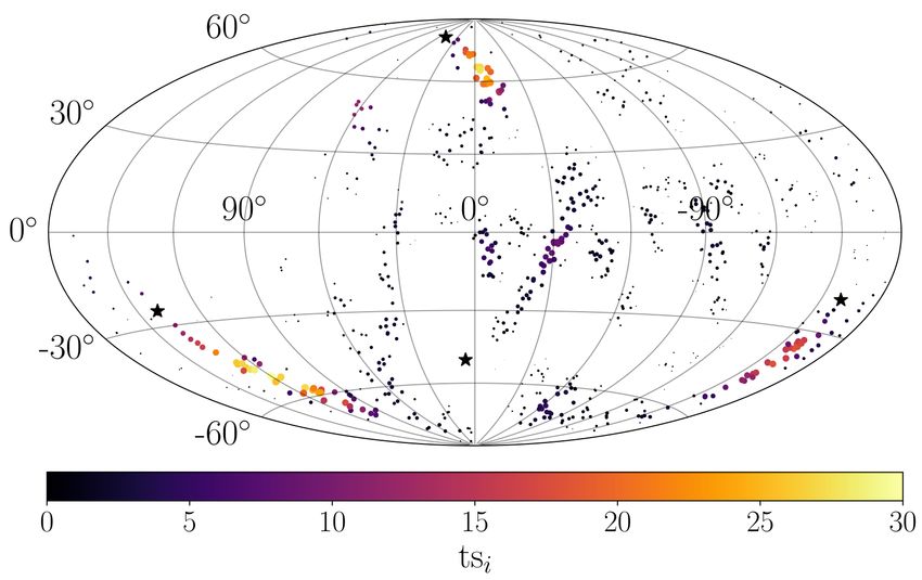
2         Marcus Wirtz et al.: Towards extracting cosmic magnetic field structures from cosmic-ray arrival directions

Fig. 1. Concept of the COMPASS method demonstrated in an astrophysical simulation (cf. section 3). Circular symbols
mark UHECR arrival directions, short lines denote the fitted orientation of coherent alignment, and the red stars show the
directions of simulated sources. (Left) State of the system at initialization and (right) after the fit. (Top) Shapes of the elliptical
signal probability density function in green and the Gaussian background probability density function in red. (Bottom) Local
orientation of fitted alignment patterns. The color code in the lower right panel corresponds to the likelihood ratio resulting
from the signal and background density functions (see text).

astrophysical simulation where UHECR nuclei from uni-               vector field û(ϑ, ϕ) tangential to the local celestial sphere
formly distributed sources are attenuated during propa-             determines the orientation of elliptically shaped probabil-
gation in the extragalactic universe. The ability to re-            ity density functions (PDFs) that are centered on each
construct the coherent directional deflections of the GMF           cosmic-ray arrival direction. Here, ϑ and ϕ denote the po-
and the advantages of using a circular reference model in           lar angle and azimuthal angle, respectively, in a spheri-
the likelihood ratio are demonstrated in the following two          cal coordinate system. The likelihood that the distribu-
chapters. Finally, the sensitivity of the method is inves-          tion of neighboring arrival directions is better described
tigated for both simulations, the simplified patterns, and          by an elliptical PDF than by a background hypothesis is
the astrophysical universe.                                         then evaluated to optimize the orientation of the ellipses’
                                                                    major axes for all cosmic-ray events in one single step.
                                                                    In this way, the vector field û(ϑ, ϕ) locally aligns with
2 Analysis strategy                                                 elongated structures which are expected to occur from
                                                                    UHECR deflections in the GMF1 . Technically, a likelihood
                                                                    ratio (cf. equation (14)) serves as an objective function in
The objective of the COMPASS method is to find align-
                                                                      1
ment patterns in UHECR arrival directions simultane-                     An intuitive analogy for the concept is the alignment of
ously across the entire sky. In this approach, an adjustable        iron filings in magnetic fields.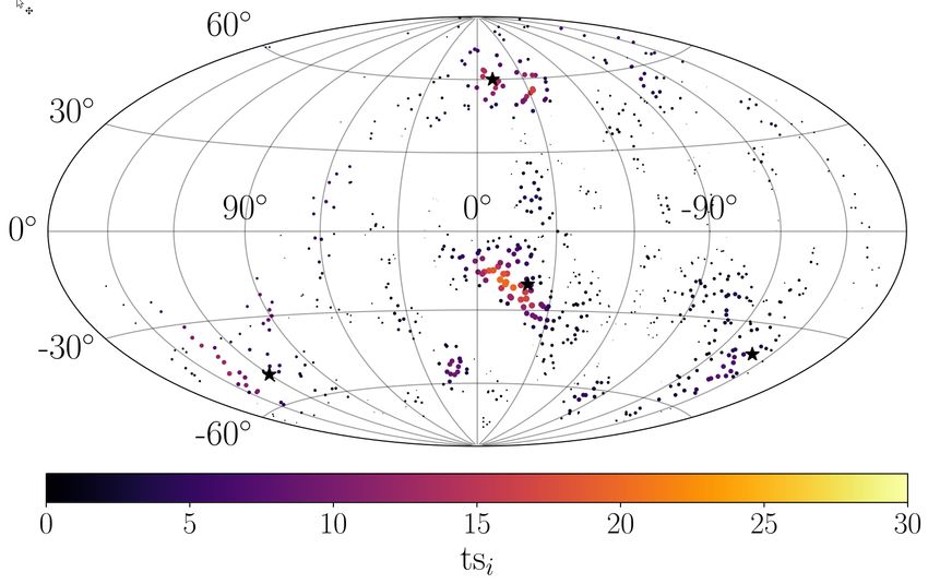
Marcus Wirtz et al.: Towards extracting cosmic magnetic field structures from cosmic-ray arrival directions            3

a minimization based on gradient descent. Additional con-         Rapid variations on small angular scales can be suppressed
straints within the analysis can be accounted for by adding       by demanding the order k of the spherical harmonics ex-
a corresponding penalization term to the objective func-          pansion to have an upper limit of k = 5. Typical examples
tion.                                                             for this value k used in the analysis are k = 4 and k = 5
    The basic concept of the COMPASS method is demon-             which yield 25 and 36 free fit parameters, respectively. The
strated in Fig. 1 where the initial state of the system is        resulting modification Ψ for a certain direction r̂ is then
shown in the left panel and the fitted state in the right         described by a rotation of û0 around the axis r̂:
panel. Here, the initialization of the vector field û(ϑ, ϕ) is
equal to the local unit vector êϑ . The upper panel shows                û(ϑ, ϕ) = R(r̂(ϑ, ϕ), Ψ (ϑ, ϕ)) û0 (r̂(ϑ, ϕ)) ,   (2)
the ellipsoidal PDF (green) and a corresponding Gaussian
background PDF (red). One can see that the orientation            where the two arguments of the rotation matrix R are
of the ellipse has changed after the fit where an alignment       the rotation axis and angle, respectively. Note that here
with a prominent pattern originating from the red marked          the polar angle ϑ is defined as being consistent with the
source is clearly visible. Additionally, the lower panel in-      Galactic latitude b; thus, in Cartesian coordinates r̂ is
dicates the orientation of the adjusted vector field û(ϑ, ϕ)     given by:
in the vicinity of the pattern. The orientation has changed
considerably only for the cosmic-ray events which are part                r̂(ϑ, ϕ) = (cos ϑ cos ϕ, cos ϑ sin ϕ, sin ϑ)T       (3)
of the pattern, whereas the ellipses of most of the isotropic
events have not changed substantially during the fit. This            For the initialized vector field û0 (r̂), three approaches
finding is also visualized by the color-coded likelihood ra-      were investigated in this work. The hairy ball theorem
tio where high values are found only for events that are          states that there exists no nonvanishing continuous tan-
part of the pattern.                                              gent vector field on the surface of the three-dimensional
    The method requires a high number of fit parameters,          sphere [20]. Thus, û0 always exhibits at least one region on
both for the parameterization of the vector field û(ϑ, ϕ)        the sphere where the vector field either radially diverges
and the UHECR model for the likelihood ratio. For the an-         at a certain point or where it circularly curls around it.
alyzed simulated data set of UHECRs with energies above           The following three initializations were used:
40 EeV, the number of free fit parameters is of the or-            – JF12 GMF: An intuitive approach is to initialize the
der of O(1000). Our method uses the software package                 fit with the best guess of the pattern orientations, e.g.
TensorFlow [16] to perform a gradient descent-based op-              the predictions of the currently most reliable GMF
timization in this high dimensional parameter space. To              model, namely that developed by Jansson & Farrar [21]
enable the computation of gradients within the scope of              (JF12). Here, to obtain the local direction of deflection
the backpropagation technique used in the field of ma-               in the direction of r̂, a magnetically highly rigid par-
chine learning, all operations of this analysis (cf. following       ticle of 1020 eV is backtracked, leaving the Galaxy in
subsections) — spherical harmonics expansion, parame-                direction r̂ 0 . Then, the local tangent vector field is de-
terization of density functions, vector algebra operations,          fined as û0 (r̂) = r̂ × (r̂ × r̂ 0 )/C where C is determined
likelihood ratio — were written with the TensorFlow API.             by the normalization according to ||û0 || = 1.
                                                                   – Galactic meridians: Here, the local tangent vector
                                                                     û0 (r̂) is equal to the local spherical unit vector êϑ in
2.1 Tangent vector field
                                                                     the Galactic coordinate system. The advantage of this
A particular challenge is the parameterization of the tan-           initialization is that it is independent of a certain GMF
gent vector field û(ϑ, ϕ) which is meant to describe the            model, while an overall symmetry with respect to the
orientation of deflection patterns caused by the GMF. The            Galactic plane is still maintained. Additionally, certain
large-scale component of the GMF is most likely respon-              models favor a general deflection preference towards
sible for patterns of coherent deflection [18, 19]. Thus, the        the Galactic plane [22], which is approximately realized
orientation of patterns is expected to vary only slightly            in this case.
within a local domain of the sky.                                  – Equatorial meridians: In analogy to the Galactic
    Here, the adaptable vector field is first realized by a          meridians, here the initialization is equal to the unit
constant vector field û0 (ϑ, ϕ) which serves as an initial-         vector êθ in the Equatorial coordinate system. This
ization and is then modified locally by an angle Ψ (ϑ, ϕ).           initialization has the advantage that one of the two
To preserve the local coherence of the resulting vector              points of divergence is located in the blind region of a
field û(ϑ, ϕ), the modification angle is parameterized by           ground-based Observatory. Here, it is used only as a
a spherical harmonics expansion of order k:                          crosscheck for the fit reliability.

                          k `                                         A visualization of the three tangent vector field initial-
                                                                  izations û0 is presented in Fig. 2. Regions with curls or
                          X X
             Ψ (ϑ, ϕ) =              am   m
                                      ` Y` (ϑ, ϕ) ,        (1)
                          `=0 m=−`
                                                                  divergences of the vector field can be seen in all three
                                                                  initializations. At these locations, the analysis exhibits
where Y`m (ϑ, ϕ) are the spherical harmonics functions and        a decreased sensitivity to find locally aligned structures
am` represent a set of free fit parameters to model any con-      as the underlying vector field û0 cannot describe them.
tinuous differentiable function on the surface of the sphere.     For the initialization of JF12 GMF, two of these features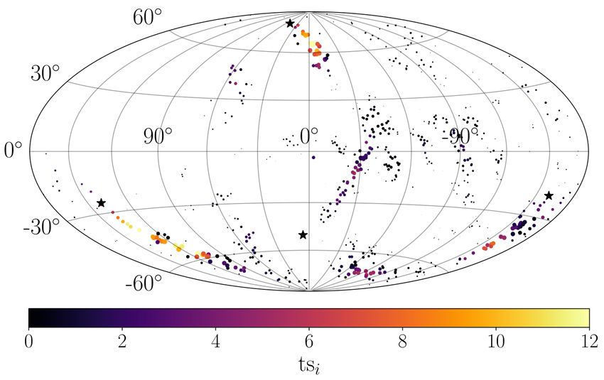
4 Marcus Wirtz et al.: Towards extracting cosmic magnetic field structures from cosmic-ray arrival directions
field û may be directly defined in the form of vector spher-
ical harmonics (VSH) [23]. In this way, positions of curls
and divergences of the vector field can be shifted dynami-
cally over the sky during the fit. Thus, they will likely stall
in sky regions without noteworthy contributions to the
likelihood ratio, i.e. in regions without prominent align-
ment patterns.
2.2 Maximum likelihood ratio
The COMPASS method evaluates the distribution of ar-
rival directions around each cosmic-ray event i in order to
search for the existence of an elongated structure. Here,
the likelihood is defined in analogy to the approach in
[24]: the total UHECR sky model consists of a sum of a
signal part E(r̂) Si (r̂) (with the contribution |fi |) which
captures elongated patterns and a purely isotropic part
E(r̂) which represents the geometrical exposure of the ob-
servatory [25]. This likelihood log(LSi ) is then compared
to a suitable reference model by calculating the likelihood
ratio. The fundamental difference with respect to the ap-
proach in [24] is that each cosmic-ray event i provides a
separate density function Si (r̂) including a fit parameter
fi which describes the contribution of the respective event
to the log-likelihood as:
N
Xtot h
log(LSi ) = log |fi | × E(Θ̂ j ) Si (Θ̂ j )
j (5)
i
+(1 − |fi |) × E(Θ̂ j ) ,
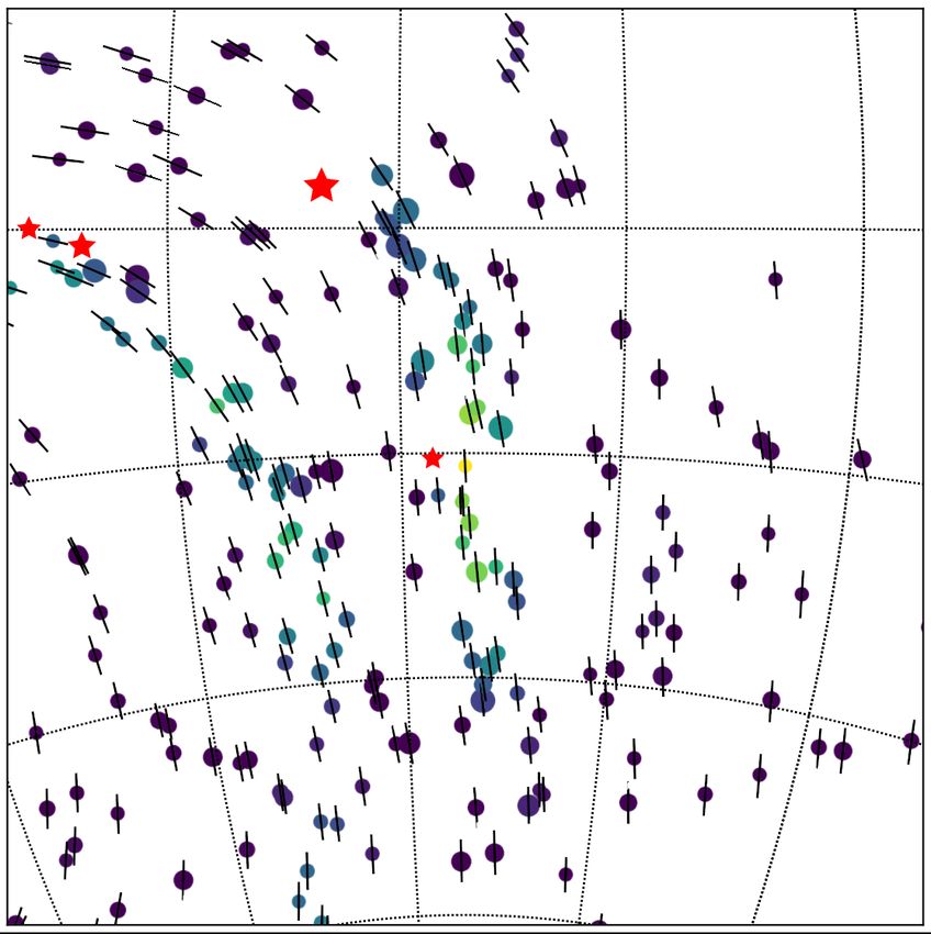
Fig. 2. Visualization of the utilized tangent vector fields û0
in the Galactic coordinate system. (Top) Local orientation of
deflection patterns from simulations in the JF12 field calcu- where Ntot is the total number of events in the data
lated by the displacement of an R = 1020 eV particle. (Mid- set and Θ̂ j the unit vector of the arrival direction of cos-
dle) Meridians in Galactic coordinates along the local êϑ unit mic ray j. Here, the signal and background contributions,
vector. (Bottom) Meridians in Equatorial coordinates. E(r̂) Si (r̂) and E(r̂), are normalized over the surface A of
the sphere:
are visible at Galactic coordinates (l, b) ≈ (90◦ , 0◦ ) and ZZ ZZ
(l, b) ≈ (−60◦ , −20◦ ). The Galactic and equatorial meridi- E(r̂) dA = 1 and E(r̂) Si (r̂) dA = 1 . (6)
ans initializations exhibit two divergences at the northern A A
and southern poles of the respective coordinate system.
An example of the working principle of the modification The set of fi represents a total number of Ntot free
function Ψ (ϑ, ϕ) for the Galactic meridians initialization fit parameters which are initialized with a value close to
is shown in the lower panel of Fig. 1. zero. Thus, the total number of free parameters of the
For the JF12 GMF initialization — depending on the COMPASS method is nfit = (k+1)2 +Ntot , where the (k+
reliability of the model predictions — it may be beneficial 1)2 part comes from the spherical harmonics coefficients
for the sensitivity to include a penalization term for large am` .
model deviations in the objective function. This penaliza- The signal part Si (r̂) of equation (5) is constructed
tion can be achieved by limiting the integrated squared as an elliptically shaped density function which is cen-
amplitude of Ψ over the entire celestial sphere as: tered at cosmic-ray direction Θ̂ i . The major axis is aligned
with the local direction of the tangent vector field ûi ≡
û(ϑi , ϕi ). Since the GMF is not well known, there is no
Z 2π Z π/2
1 accurate mathematical description for the expected shape
F = Ψ 2 (ϑ, ϕ) cos(ϑ) dϑ dϕ . (4)
4π 0 −π/2 and size of a deflection pattern. Here, the density func-
tion Si is parameterized on the basis of a non-symmetrical
As a potential improvement in scenarios where many Gaussian distribution where the width follows an ellipse
directions exhibit alignment patterns, the tangent vector equation as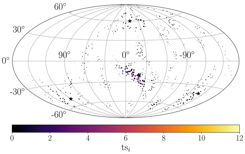
Marcus Wirtz et al.: Towards extracting cosmic magnetic field structures from cosmic-ray arrival directions                      5

                                                               !
                    (r̂ · ûi )2   (r̂ · (Θ̂ i × ûi ))2
 Si (r̂) = C × exp − 2           −           2                     , (7)
                      δmax                 δmin

    for all directions r̂ located in the same hemisphere as
cosmic ray i, i.e. Θ̂ i · r̂ ≥ 0. In the opposite hemisphere of
the sky the density function is set to zero. The hyperpa-
rameters δmax and δmin denote the angular extent in the
direction of the ellipses’ semi-major and semi-minor axes,
respectively. C denotes a normalization factor which is in-
vestigated in section 2.3.
                                                        ⊥
    For every cosmic ray i, the minimal distance δi,j      be-
tween the direction Θ̂ j of the neighboring cosmic ray j
and the orthodrome ζ, as defined by Θ̂ i and ûi , is given
by the relation:

                      ⊥           Θ̂ j · (Θ̂ i × ûi )
                 sin(δi,j )=                             .           (8)
                                      ||Θ̂ i × ûi ||

     Since Θ̂ i and ûi are unit vectors, the term ||Θ̂ i × ûi ||
is equal to one. Thus, the numerator of the second term in
the exponential function of equation (7) can be identified
as the transverse displacement of cosmic-ray direction Θ̂ j
relative to the fitted orientation ûi . Likewise, the great-
circle distance along the orthodrome ζ – and therefore
                                                            k
along the pattern orientation — is given by sin(δi,j ) =
Θ̂ j · ûi . Thus, for small angles, i.e. sin δi,j ≈ δi,j , equa-
tion (7) can be identified as a two-dimensional Gaussian
distribution on the sphere where contour lines of equal
function values Si follow an ellipse equation:

                   k
                         !2                  !2
                  δi,j                 ⊥
                                      δi,j
                              +                   = const .          (9)
                 δmax                 δmin

    For the reference model of the likelihood ratio, two
approaches were explored in this work: a purely isotropic
hypothesis following the geometrical exposure E(r̂) and a
Gaussian reference model with identical signal strength fi
(compared to the elliptical ones) to cancel out overdensi-
ties.

 – Isotropic reference model E(r̂): The highest sen-                       Fig. 3. Normalized probability density distributions for (top)
   sitivity to reject an isotropic scenario is obtained by                 signal part Si (r̂), (middle) the Gaussian reference part Gi (r̂),
                                                                           and (bottom) the geometrical exposure E(r̂). For the signal and
   testing explicitly against this hypothesis in the likeli-
   hood ratio. Thus, each cosmic ray i provides the same                   Gaussian reference parts, the cosmic-ray direction Θ̂ i is cen-
                                                                           tered at Galactic coordinates ϑ = 0◦ and ϕ = 0◦ and the ellipse
   log-likelihood contribution:
                                                                           geometry is δmax = 30◦ and δmin = 10◦ where the major axis
                                      Ntot
                                                                           is aligned with the êϑ unit vector. The geometrical exposure is
                                                                           given by the geometry of the Pierre Auger Observatory with a
                                      X
                   log(LR
                        i )       =          log(E(Θ̂ j )) ,        (10)
                                                                           maximum zenith angle of 80◦ .
                                       j

 – Gaussian reference model Gi (r̂): Here, the refer-
   ence model is provided by equation (7) where
                                             √ both the
   major axis and minor axis radii are set to δmax × δmin
   with respect to the ellipse dimensions of the signal dis-
   tribution. By choosing the geometric average of both
   dimensions, the effective solid angle of the symmetric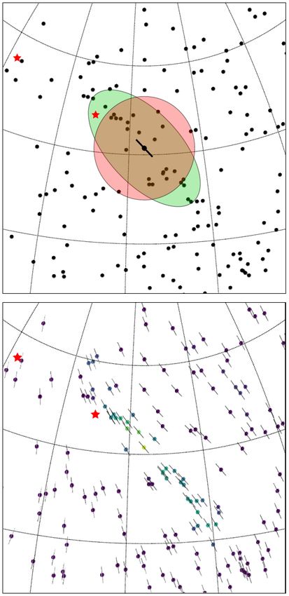
6        Marcus Wirtz et al.: Towards extracting cosmic magnetic field structures from cosmic-ray arrival directions

    reference model is unchanged and equation (7) can be
    written as a symmetric Gaussian-like distribution:                        0.175
                                                                                                                             α = 0◦
                                                    !                                                                        α = 30◦
                              sin2 ( ^(r̂, Θ̂ i ) )                           0.150
          Gi (r̂) = C × exp −                         . (11)                                                                 α = 60◦
                                δmax × δmin                                   0.125                                          α = 90◦
    In the log-likelihood ratio, the same value for the con-                                                                 E(δ)

                                                                        1/C
                                                                              0.100
    tribution fi as in equation (5) is chosen to evaluate
    solely the difference between an elliptically shaped and                  0.075
    a symmetrical pattern:
                                                                              0.050
                   N tot       h
                                                                              0.025
                   X
       log(LR
            i )=           log |fi | × E(Θ̂ j ) Gi (Θ̂ j )
                     j                                           (12)         0.000
                                                             i
                                                                                  −90   −60       −30       0        30       60       90
                                   +(1 − |fi |) × E(Θ̂ j ) ,
                                                                                                        δ / deg
    During the TensorFlow fit, the gradient of fi is com-
                                                                        Fig. 4. Integral 1/C of exposure-folded Gaussian probability
    puted only with respect to the signal contribution in               distribution as a function of the equatorial declination δ for the
    equation (5) in order to prevent active adaption of the             center direction of the ellipse. The semi-major and semi-minor
    reference model R.                                                  axis are δmax = 30◦ and δmin = 10◦ , respectively. Colored lines
    Examples of the normalized probability density func-                denote different ellipse orientations α. The black dashed line
tion of the elliptically shaped signal part S(r̂), the sym-             indicates the probability density function value of the normal-
metric reference part G(r̂), and the geometrical exposure               ized exposure E(δ).
E(r̂) are visualized in Fig. 3.
    For the objective function of the fit, each cosmic ray
contributes with a separate log-likelihood ratio tsi as:                the objective function J with respect to the parameters.
                                                                        As an optimizer for the minimization problem, RMSProp
              tsi = 2 × [ log(LSi ) − log(LR                            [27] is used, which supports an efficient optimization for
                                           i )] .                (13)
                                                                        adaptive parameters of different magnitudes. This is real-
    For an isotropic arrival distribution, each individual tsi          ized by allowing each adaptive parameter to have a sepa-
follows a χ2 distribution with the degrees of freedom cor-              rate step size which is increased (decreased) depending on
responding to the free fit parameters according to Wilks’               a consistent (inconsistent) direction of the gradient with
theorem [26]. Therefore, the corresponding sum of all indi-             respect to the parameter in two consecutive update steps.
vidual test-statistic contributions is Gaussian distributed             For stability reasons, the optimizer was complemented by
according to the central limit theorem. The latter state-               additional conditions for the learning rate adaption.
ment holds only if the individual contributions are inde-
pendent of each other, which is not entirely the case in
this application since the density functions of neighbor-               2.3 Normalization
ing cosmic rays overlap. Nevertheless, it has been explic-
itly checked in Monte Carlo simulations of isotropic   P ar-   The normalization factor C in equation (7) is generally
rival distributions that the summed test statistics i tsi
                                                               determined by equation (6) and requires a numerical in-
approximately follows a Gaussian distribution. Thus, the
                                                               tegration for a non-uniform geometrical exposure E(r̂).
average test statistic htsi provides a well-defined metric to
                                                               Since the exposure E(r̂) = E(δ(r̂)) depends only on the
evaluate the pattern alignment over the entire sphere:
                                                               equatorial declination δ [25], the surface integral of the
                             1 X
                                 N                             term E(δ) Si (r̂) depends only on the center direction Θ̂ i
                      htsi =         tsi .                (14) of the ellipse and its relative orientation |αi | towards the
                             N i                               local spherical unit vector êδ in equatorial coordinates.
                                                               As ûi determines the orientation of the ellipse Si (r̂), the
To maximize equation (14), the negative average test statis- angle α is defined by cos α = û · ê .
                                                                       i                       i    i   δ
tic is chosen as the objective function for the gradient           The exposure-weighted integral for an ellipse with di-
descent. Additionally, in the case of the JF12 GMF ini- mensions (δ                             ◦  ◦
                                                                            max , δmin ) = (30 , 10 ) is visualized as a func-
tialization of the tangent vector field, the objective term F tion of the equatorial     declination δ of the center direction
from equation (4) is added. Thus, the total objective func- and for different values of α in Fig. 4. It can be seen
tion J exhibits one hyperparameter λF which represents that the inverse normalizationi factor 1/C approaches the
the confidence in the GMF model:                               probability density function value of the exposure E(δ) for
                                                                                                             ◦           ◦
                     J = −htsi + λF · F .                 (15) intermediate equatorial declinations −60 < δ < 20 . In
                                                               the border regions of the geometrical exposure, the inte-
For the gradient descent, the fit parameters fi and am   ` are gral is larger than the respective exposure values due to
adapted simultaneously by calculating the derivative of the extent of the elliptical distribution. For the gradient
Marcus Wirtz et al.: Towards extracting cosmic magnetic field structures from cosmic-ray arrival directions 7
descent, the normalization factor was calculated for a grid
of equatorial declinations δ and orientations α and then
interpolated linearly between the grid points.
3 Benchmark simulations
The sensitivity of the COMPASS fit method is evaluated
in two different benchmark simulations. Proof of concept
is given on the basis of a simple four-source model where
each source contributes an equal number Ns of cosmic
rays. The second benchmark extends an astrophysical sim-
ulation of an extragalactic source population [28] by de-
flections in the GMF and the observational exposure E(r̂).
Therefore, given a certain source density, it provides the
most reasonable estimate of the sensitivity. Both simu-
lations mimic the current data set of the Pierre Auger
Observatory for anisotropy studies (e.g. [17]) above ener-
gies of 40 EeV with a total event number of Ntot = 1119
and zenith angles up to 80◦ .
Benchmark 1: Distinct source scenario
The first benchmark simulation consists of UHECRs Fig. 5. Construction of benchmark 1 scenario consisting of
with energies E that follow the parameterized power law four distinct sources, in the Galactic coordinate system. Each
from [29] above an energy threshold of 40 EeV. The nu- of the four sources (black star symbols) contributes Ns = 20
clear charges are assumed to be energy-independent and source events with color coded charge number Z. (Top) Con-
uniformly distributed between Z = 1 and Z = 8. While Ns struction of implementing GMF uncertainties for the source
out of the Ntot = 1119 UHECR events are assigned to each events. (Bottom) Complete simulations of 80 source events and
of four different, randomly placed point-like sources in the 1039 isotropically distributed arrival directions.
sky, the remaining cosmic rays are distributed isotropi-
cally, following the geometrical exposure E(r̂) of the ex-
periment. the lower panel of Fig. 5.
The deflections in the GMF are simulated as follows:
First, the cosmic rays with magnetic rigidity R = E/Z are Benchmark 2: Astrophysical simulation
propagated through the large-scale component of the JF12
model using a magnetic field lens [6, 30]. Next, a rigidity- The second benchmark simulation is based on results
dependent Gaussian smearing of δ = 0.5 × Z/E [EeV] rad obtained in a combined fit of the UHECR observables at
is applied which corresponds approximately to the median the Pierre Auger Observatory [31] and their anisotropy im-
scattering angle in the JF12 random and striated fields. A plications for given source densities following [28]. Here,
visualization of the arrival directions of this step is shown source candidates are uniformly distributed in the uni-
for Ns = 20 source events as black circles in the upper verse following a source density ρS which results in aniso-
panel of Fig. 5. tropies due to attenuation effects during the propagation.
If the JF12 GMF initialization is chosen in the fit The deflection in the GMF is applied in the same
method, we additionally apply a shift of arrival directions way as for the benchmark 1 scenario by using the JF12
to mimic the uncertainties in the GMF model. Here, the model and a rigidity-dependent Gaussian smearing of δ =
entire pattern of source m is modified by a spherical angle 0.5 × Z/E [EeV] rad. The relative arrival probability for
Ψ̃m performed by a rotation of the individual cosmic-ray different extragalactic directions and rigidities caused by
arrival directions Θ̂ i from source m around its direction the GMF (e.g. [22]) are accounted for. The relative obser-
r̂ m by the angle Ψ̃m . The construction of this rotation is vation probability resulting from the geometrical exposure
sketched by the dotted line in the top panel of Fig. 5. of the observatory is likewise accounted for. Fig. 6 shows
For the four sources, spherical angles Ψ̃m are selected in the resulting arrival directions of the benchmark 2 simula-
good accordance with uncertainties between existing GMF tion for a source density of ρS = 10−2 Mpc−3 . The circu-
models [18], as examples Ψ̃1 = −30◦ , Ψ̃2 = 0◦ , Ψ̃3 = +45◦ lar symbols denote cosmic-ray arrival directions, the color
and Ψ̃4 = +15◦ in order of the ascending Galactic longi- scale corresponds to the nuclear charge Z, and the gray
tude l (from right to left in the upper panel of Fig. 5). The shaded events originate from sources which contribute at
colored symbols indicate the resulting arrival directions af- least three cosmic rays. One can see that patterns may
ter this displacement. All arrival directions, consisting of occur in multiple regions of the sky with strongly varying
80 source events and 1039 isotropic events, are shown in event contributions attributable mainly to the source dis-8 Marcus Wirtz et al.: Towards extracting cosmic magnetic field structures from cosmic-ray arrival directions
Fig. 6. Example of benchmark 2 scenario consisting of an as- Fig. 7. Visualization of the modification angles Ψ (ϑ, ϕ) (color-
trophysical simulation including deflection in the JF12 model coded) which is defined relative to the JF12 model (JF12 GMF
for the GMF. Cosmic rays originate from uniformly distributed initialization for û0 ) after a fit to benchmark 1 scenario with
sources of density ρS = 10−2 Mpc−3 and are attenuated by Ns = 20 source events. Gray circles denote cosmic rays that
extragalactic photon fields. Gray shaded events denote cosmic originate from one of the four sources and the dotted lines mark
rays which originate from a source with at least three contribut- contours of 15◦ -spacing in Ψ .
ing events. For this specific source distribution the strongest
source contributes 30 cosmic rays, which corresponds to the
median value of 1000 simulated universes for this source den-
sity. The star symbols denote source directions where the size sky regions where a significant pattern is found. Hence, for
is proportional to the cosmic-ray contribution. The skymap is the benchmark 1 simulation, the final angle Ψi ≡ Ψ (ϑi , ϕi )
shown in the Galactic coordinate system. of cosmic rays i which originate from one of the simu-
lated sources m is expected to approach the simulated
uncertainty Ψ̃m . Here, the necessary correction is mod-
tance. Some sources situated outside the visible sky of the eled by the spherical angles Ψ̃m for the four sources where
observatory (e.g. source at Galactic coordinates l ≈ 110◦ Ψ̃1 = −30◦ , Ψ̃2 = 0◦ , Ψ̃3 = +45◦ and Ψ̃4 = +15◦ are
and b ≈ 50◦ ) still contribute a substantial fraction of cos- chosen (cf. section 3). Note that a non-linear deflection
mic rays due to coherent deflection in the GMF. behavior in the GMF may disturb the correct values of
Additionally, if the tangent vector field is initialized as Ψ̃m . This effect is particularly strong for cosmic rays with
JF12 GMF, again, an uncertainty angle Ψ̃ for the GMF a low rigidity Ei /Zi , i.e. for high absolute deflection angles
is simulated. To conserve consistent deflection patterns of with respect to their source.
sources in similar directions of the sky, the uncertainty Here, for the first application of the fit, the order of
Ψ̃ (r̂) = Ψ̃a r̂ · d̂i is modeled as a dipolar function with the spherical harmonics expansion of equation (1) is de-
amplitude Ψ̃a = 45◦ and random direction of the dipole fined as k = 5, which corresponds to 36 free fit param-
maximum d̂i for each simulated universe i. eters. In this case, modifications of the GMF model can
This simulation of the UHECR universe exhibits only be performed coherently in sky regions that have angu-
one single free parameter, the source density ρS , which lar scales above the order of 180◦ /k = 36◦ . The degree
directly determines the degree of anisotropy in the arrival of modification Ψ itself is constrained by the hyperpa-
directions. The higher the source density, the more sources rameter in the objective function (15) where a value of
are within a horizon where attenuations do not play an λF = 1 is chosen for this purpose. For the ellipse geome-
important role and, therefore, the more isotropic the sky try, values of (δmax , δmin ) = (10◦ , 5◦ ) are chosen in equa-
is. tion (7). Furthermore, the Gaussian reference model from
equation (12) was selected for the √ likelihood ratio where
the effective Gaussian width is 10◦ × 5◦ ≈ 7.1◦ .
4 Reconstruction of the Galactic magnetic The fitted modification function Ψ (θ, ϕ) is visualized
field in Fig. 7 together with the cosmic rays that originate from
the simulated source candidates. As an overall impression
In this section, proof of concept is provided by showing the color code in the vicinity of the source candidates m
that the orientation of patterns can be correctly recon- agrees with the simulated uncertainties Ψ̃m . To quantify
structed based on the benchmark 1 simulation from sec- the method’s reconstruction abilities, for each source m
tion 3. the fitted Ψi for the 10 closest cosmic rays that originate
During the minimization process, the modification an- from the source are averaged. The corresponding averaged
gle Ψ (ϑ, ϕ) rotates the ellipses of the signal hypothesis of values are hΨ1 i = (−32 ± 1)◦ , hΨ2 i = (6 ± 2)◦ , hΨ3 i =
equation (1) such that they align with elongated patterns (+47 ± 5)◦ and hΨ4 i = (+15 ± 5)◦ , which are in good
in the cosmic-ray arrival direction distribution. For the agreement with the simulated uncertainties Ψ̃m .
JF12 GMF initialized vector field û0 , the angle Ψ (ϑ, ϕ) The next step is to investigate if orientations of pat-
corresponds directly to a correction of the JF12 model in terns as simulated with the JF12 model can also be cap-Marcus Wirtz et al.: Towards extracting cosmic magnetic field structures from cosmic-ray arrival directions 9
60◦ 5 Reference model of the likelihood ratio
30◦ In this section, two different choices of the reference model
(cf. section 2) for the likelihood ratio as defined in equa-
90◦ 0◦ -90◦ tion (13) are studied: the isotropic model E which follows
0◦
the geometrical exposure of an experiment, and the Gaus-
sian model Gi with identical signal contributions fi as
-30◦ assigned to the elliptically shaped signal model Si . Again,
the ellipse geometry is defined as (δmax , δmin ) = (10◦ , 5◦ ),
-60◦ the initialization for û0 is Galactic meridians, the spher-
ical harmonics order is k = 4, and the hyperparameter
Fig. 8. Visualization of the tangent vector field û(Θi ) (black λF = 0. To obtain an impression of the performance over
lines) of equation (2) using the Galactic meridians initializa-
the sky, it is useful to investigate the individual test statis-
tion of û0 (r̂). Black star symbols show the simulated source
tics tsi defined in equation (13) as well as the anticipated
directions while the red circular symbols mark the Ns = 20
events per source which have been displaced by the JF12 model
signal contribution fi from equation (5).
without simulated GMF uncertainties.
Isotropic reference model E
The resulting test statistics tsi after the fit using the
isotropic reference model (cf. equation (10)) is shown in
tured without including information on the explicit GMF the left panel of Fig. 9. The fit results of the benchmark 1
model. For this purpose, we chose the Galactic meridians simulation are displayed in the upper panel with Ns = 20
initialization of û0 where initial ellipse orientations are source events in each of the four patterns. The fitted signal
aligned with the local spherical unit vector êϑ of the lati- contribution fi for the events i are proportional to the size
tude in the Galactic coordinate system. Since no informa- of the circular symbols where a common normalization
tion on the simulated GMF is included, the penalization among all four figures is chosen.
factor of equation (15) is not required and is therefore set Clearly, for benchmark 1 scenario in the upper panel,
to λF = 0. Thus, the tangent vector field can be rotated the patterns produced by the four simulated sources ex-
by the angle Ψ (θ, ϕ) without constraint. For this setup, hibit cosmic rays with a substantially larger test statistic
the degree of the spherical harmonics expansion was de- tsi compared to the isotropically distributed background
creased to k = 4 to avoid rapid changes of Ψ on small events. Accordingly, the anticipated signal contribution fi
angular scales. The order k of the spherical harmonics ex- of the source events is larger, as shown by the size of the
pansion is the most challenging free parameter since the markers. Some local clusters of events with test statis-
optimal choice depends on the angular scale of domains tics tsi > 0 can also be found in the isotropically dis-
with a coherent GMF deflection. While more complex pat- tributed background events, however, with considerably
terns can generally be fitted with an increasing order of smaller values of both the test statistic tsi and the sig-
k, these structures are more difficult to interpret. nal contribution fi . The average test statistic from equa-
tion (14) is htsi ≈ 1.6. The highest signal fractions reach
A visualization of the fitted tangent vector field û(Θi ) values of about fi = 1.4%, which is in good agreement
for each individual cosmic-ray arrival direction Θi is pre- with the 20 of 1119 injected signal cosmic rays per source.
sented in Fig. 8 where the source events are highlighted Note that the complete signal contribution of 20/1119 ≈
in red. All four deflection patterns in this simulation were 1.8% is not necessarily reached even for the innermost cos-
successfully captured by an alignment of the tangent vec- mic ray of the pattern due to fluctuations in the isotropic
tor field û(r̂) along the local track of source events. There background and the ellipse’s limited extent of 10◦ in the
is also structure visible in sky regions without source con- semi-major axis, which is mostly less than the extent of
tribution where fluctuations of isotropically distributed the pattern.
arrival directions were connected along their most promi- To assess the impact of solely overdense but not elon-
nent patterns. In the sky region at Galactic coordinates gated structures on the test statistic, a new simulation is
(l, b) ≈ (−90◦ , −75◦ ) the isotropic fluctuation was even studied which again consists of four sources each emitting
strong enough to rotate the initialized tangent vector field 20 cosmic rays. Instead of simulating deflections in the
û0 by up to 95◦ . This suggests that arbitrarily oriented GMF, the source events are drawn from a Fisher distri-
alignment patterns of cosmic-ray arrival directions can be bution [32] of a width of 10◦ centered on the direction of
captured even when oriented orthogonally with respect to the source. Here, to enable a better comparison between
the chosen initialization û0 . both scenarios, the source directions were approximately
centered within the resulting arrival patterns of the bench-
To assess whether a fitted pattern is caused by isotropic mark 1 simulation.
fluctuations, the individual cosmic-ray test statistics from As shown in the lower panel of Fig. 9, the method also
equation (13) have to be compared to those found in responds with high individual test statistics tsi and an-
isotropic skies. These sensitivity studies are presented in ticipated signal contributions fi due to the event excess
section 6. of Ns = 20 relative to an isotropic expectation. However,10 Marcus Wirtz et al.: Towards extracting cosmic magnetic field structures from cosmic-ray arrival directions
Fig. 9. Comparison of fit performance for (left) isotropic E and (right) Gaussian reference model Gi , in Galactic coordinates.
(Top) Benchmark 1 simulation from section 3 with Ns = 20 events per source and deflection in the JF12 model. (Bottom)
Gaussian overdensity with a cluster of Ns = 20 events distributed around the star symbols with a Gaussian width of 10◦ and
without GMF deflection. The color code of each event i corresponds to the individual test statistic tsi . The size of the circular
symbols is proportional to the signal contribution fi with identical normalization among all four figures.
for three of the four Fisher distributions the resulting test visible. Thus, the purity of detected patterns is increased
statistics are much smaller than in the case of the bench- compared to when the isotropic reference model was used.
mark 1 simulation.
Again, the response to Gaussian overdensities is as-
sessed in the bottom panel of Fig. 9 with four Fisher-
Gaussian reference model Gi
distributed event clusters of 10◦ Gaussian width. Since
the Gaussian-shaped event structures are well described
The right panel of Fig. 9 again shows the individual by the Gaussian reference hypothesis Gi , there is a sig-
test statistic tsi (color coded) and the fitted signal contri- nificant loss in the test statistic for the overdense sky re-
butions fi (size of circles) for the Gaussian reference hy- gions compared to when the isotropic reference E is used.
pothesis Gi as defined in equation (12). For the benchmark In the vicinity of three Gaussian event clusters, there is
1 simulation in the upper panel, the anticipated signal con- only barely more fitted signal contribution fi compared
tribution fi is approximately equal to the case where the to the remaining sky. The individual test statistics tsi vis-
isotropic reference model E was chosen, as can be esti- ibly deviates from natural isotropic fluctuations only for
mated from the size of the markers. However, while in the the events of one of the Gaussian clusters, namely at co-
case of the isotropic reference model both the event excess ordinates (l, b) = (−20◦ , −20◦ ).
and the elongation of the structure contributed to the test
statistic, for the Gaussian reference model only the latter As there are already known event excesses in UHECR
information can be used. Thus, on the one hand, the over- data, e.g. in data of the Pierre Auger Observatory for this
all scale of the individual test statistics tsi is much smaller, energy threshold (e.g. [24, 33]), there is a risk of detecting
as reflected by the color scale. Therefore, the average test these features again rather than new elongated structures
statistic of equation (14) drops to htsi ≈ 0.8. On the other when using the isotropic reference model E. Therefore, in
hand, since there is no sensitivity to overdense regions, the following we use the Gaussian-like reference model Gi
some of the patterns that were caused by fluctuations of where the effects of overdensities are mostly canceled out
isotropically distributed background events are no longer by the likelihood ratio.Marcus Wirtz et al.: Towards extracting cosmic magnetic field structures from cosmic-ray arrival directions 11
Fig. 11. Distribution of average test statistic htsiiso for 104
Fig. 10. Distribution of individual test statistics tsi as ob- isotropic skies (gray) compared to the values obtained in the
tained in the benchmark 1 simulation (cf. upper right panel benchmark 1 simulation (vertical red lines) with Ns = 5 (solid),
of Fig. 9). The red (gray) histogram shows the contribution Ns = 10 (dashed), Ns = 15 (dash-dotted), and Ns = 20 (dot-
of the 80 source (isotropically distributed) events. The dashed ted) source events.
vertical black line denotes the average test statistic htsi of all
events in the sky.
htsi = 0.23, 0.30, 0.41, 0.72, respectively. To calculate the
chance probability pval of obtaining these average test
6 Sensitivity studies statistics from an isotropic arrival-direction distribution,
the method is additionally applied to 5 × 10⁴ isotropic
realizations of the sky which follow the geometrical ex-
In this section we investigate the sensitivity of the COM-
posure of the observatory. The distribution of the aver-
PASS method with respect to its ability to reject isotropic
age test statistics htsiiso for isotropic skies is shown as a
distributions of cosmic-ray arrival directions. According to
gray histogram in Fig. 11. While there is no isotropic sky
the findings from section 5, for the following subsections
yielding a higher average test statistic than the scenarios
the Gaussian reference model Gi (cf. equation (12)) is cho-
with Ns = 20 source events, the isotropic chance proba-
sen in the likelihood ratio. In addition, following section 4
bilities for the simulations with smaller source events are
and the studies in section 6.3, the tangent vector field û0
pval = 0.40, 0.14, 0.003, in order of increasing Ns .
is initialized along the Galactic meridians — i.e. û0 is
As expected from the central limit theorem (cf. sec-
equal to the local spherical unit vector êθ . Therefore, the
tion 2), the gray histogram shows that the average test
penalization term F in equation (15) is removed by set-
statistic htsiiso for an isotropic arrival sky approximately
ting λF = 0. For a comparison of the sensitivity with a
follows a Gaussian distribution. Thus, the sensitivity for
more classical analysis to search for elongated structures
the scenario shown in Fig. 5 with Ns = 20 source events
refer to [34].
can be estimated by fitting a Gaussian distribution to the
gray histogram. In this case, the estimated chance prob-
ability is about 3 × 10⁻¹¹ which translates to about 6.5 σ
6.1 Sensitivity for distinct source scenario standard deviations in the normal distribution.
The distribution of individual test statistics tsi as ob-
tained in the benchmark 1 simulation from section 3 is 6.2 Sensitivity for the astrophysical universe
presented in Fig. 10. As already suggested by the upper
right panel of Fig. 9, most of the events that exhibit high While the previous section provided an idea of the sen-
test statistics are attributed to one of the four sources. sitivity for comparably clear patterns with a certain sig-
In total, more than half of the source events show test nal contribution, this section evaluates the expected im-
statistics larger than 3, which, in turn, is only reached for plication for an astrophysical universe of uniformly dis-
about 5% of the isotropic events. Instead, the isotropic tributed UHECR sources. For the benchmark 2 simula-
distribution peaks close to zero, with about 50% of events tions, 300 simulated universes for each of the source den-
exhibiting test statistics smaller than 10−5 . One can of sities ρS = (10−1 , 3 × 10⁻² , 10−2 , 3 × 10⁻³ ) Mpc−3 were
course find a statistical measure to reject isotropy based investigated. The average test-statistic distribution as ob-
on the evaluation of events with a high test statistic, i.e. tained from the fit exhibits a comparably large spread,
based on the tail of the distribution in Fig. 10. However, which is consistent with the fluctuations in the degree of
it was found that the average test statistic htsi provides anisotropy. The median and 68 percentiles of the aver-
the most stable measure for various simulation setups. age test statistics for the four source densities are htsi =
In the next step, we evaluated the average test statistic 0.27+0.16 +0.39 +0.31 +1.92
−0.08 , 0.38−0.11 , 0.54−0.22 , 0.86−0.30 , respectively, as
htsi for different numbers of source events Ns = 5, 10, 15, visualized in Fig. 12. As expected, the test statistic in-
20 in the benchmark 1 simulation. As shown in Fig. 11, creases with decreasing source density as the arrival sce-
the resulting values for the average test statistics are narios become increasingly anisotropic.12 Marcus Wirtz et al.: Towards extracting cosmic magnetic field structures from cosmic-ray arrival directions
Fig. 12. Distribution of average test statistics htsiiso for 5×10⁴
isotropic skies (gray) compared with the values obtained in the
benchmark 2 simulation (vertical lines) with source densities
of ρS = 10−1 /Mpc3 (blue), ρS = 3 × 10⁻² /Mpc3 (orange),
ρS = 10−2 /Mpc3 (green), and ρS = 3 × 10⁻³ /Mpc3 (red). The
small triangles denote the 68% quantiles.
Fig. 13. Example realization of arrival directions from the
benchmark 2 simulation with a source density of ρS =
10−2 Mpc−3 . The strongest of the sources (red star symbols)
For the isotropic chance probability pval , the average at Galactic longitude l ≈ −133◦ and Galactic latitude b ≈ 14◦
test statistic is again compared to the fit results for the contributes with 29 cosmic rays. Sizes of the cosmic-ray events
5×10⁴ isotropic realizations which are shown as a gray his- (colored circles) correspond to the energy E, the color code
togram in Fig. 12. For the source densities of 10−1 Mpc−3 to the individual test statistics tsi , and the short black lines
and 3·10−2 Mpc−3 the isotropic chance probability can be indicate the tangent vector field û0 , i.e. the orientation of the
directly determined by the fraction of the gray distribu- major-axis of the ellipses.
tion that is above the corresponding test-statistic values.
Here, the chance probabilities yield pval = 0.229, 0.013
for the two source densities respectively. For the smaller 6.3 Optimization of free parameters
source densities of 10−2 Mpc−3 and 3 × 10⁻³ Mpc−3 , the
isotropic chance probability can again be estimated by In this subsection we evaluate the impact of the free
parameterizing the null hypothesis with a Gaussian dis- parameters more profoundly based on the astrophysical
tribution. In this case, the estimated values are 8.3 × 10⁻⁶ benchmark 2 simulation with a source density of ρs =
and 1.4 × 10⁻¹⁷ , respectively, which correspond to a devi- 3 × 10⁻² Mpc−3 from section 3. Firstly, the initialization
ation of 4.3 σ and 8.5 σ standard deviations in the normal method of the tangent vector field û0 and accordingly the
distribution. Thus, in the case of a result on data that is free parameter λF are addressed. Secondly, the impact
compatible with an isotropic distribution, the density of of the ellipse geometry, namely the semi-major and semi-
UHECR sources for this astrophysical model can be esti- minor axes, on the performance is studied.
mated.
Fig. 13 shows arrival directions in the sky region around 6.3.1 Confidence in the JF12 GMF initialization
the strongest individual test statistic tsi for the scenario
that exhibits the median average test statistic htsi out of The initialization of the tangent vector field û0 according
the 300 simulations with a source density of 10−2 Mpc−3 . to the predictions from the JF12 model (JF12 GMF ) is
Here, the strongest individual test statistic is tsi = 8.6 visualized in the top panel of Fig. 2. As pointed out in
and the corresponding cosmic-ray event (yellow point in section 2, depending on the reliability of the GMF model
the center of the sky patch) is part of the pattern from it may be beneficial to constrain the allowed deviations
the source at Galactic coordinates l ≈ −133◦ and b ≈ 14◦ . Ψ (ϑ, ϕ) with equation (4), since this reduces high test
Contributing with a total of 29 events, this is the strongest statistics from fluctuations in isotropic arrival distribu-
source in this realization. The orientation of the tangent tions. Therefore, the isotropic chance probability pval is
vector field û(ϑ, ϕ) (short black lines) additionally sug- investigated as a function of the free objective parameter
gests that the alignment works reasonably well even for λF in equation (15) for two reasonable estimates of the
patterns that are only separated by about 20◦ . Thus, the uncertainties in GMF models.
vector field û(ϑ, ϕ) is expected to provide an adequate The first estimate is obtained by simulating the deflec-
coherent description of the deflection in the GMF for suf- tion in the GMF with the model of Pshirkov et al. using
ficiently strong signals. an antisymmetric disk field (PT11-ASS) [35] instead ofMarcus Wirtz et al.: Towards extracting cosmic magnetic field structures from cosmic-ray arrival directions 13
Fig. 15. Scan of the ellipse geometry (δmax , δmin ) for the
Fig. 14. Scan of hyperparameter λF for the confidence in the Galactic meridians initialization and λF = 0 evaluated on the
assumed GMF model (here JF12). The initialization of the tan- astrophysical benchmark 2 simulation with source density of
gent vector field û0 follows the JF12 GMF procedure and the ρS = 3 × 10⁻² Mpc−3 . The isotropic chance probability is cal-
isotropic chance probability pval is derived for the benchmark culated with a total of 104 isotropic skies for each of the ellipse
2 simulation with a source density of ρS = 3 × 10⁻² Mpc−3 constellations.
from section 3. The red crosses show deflections in the PT11-
ASS model and the blue crosses show deflections in the JF12
model, which is modified by a dipolar modulated uncertainty isotropic chance probability pval , the analysis is applied to
angle with amplitude Ψa . a total of 104 isotropic skies for each geometry.
The resulting median chance probabilities pval of 300
sky realizations are displayed in Fig. 15 where each of
the JF12 model used in section 3. The second estimate is the five segments indicate one of the semi-major axes
given by a modification of the JF12 model with dipolar δmax . Generally, larger and less elongated ellipse sizes are
distributed modification angles of amplitude Ψa = 45◦ as beneficial for the sensitivity of the COMPASS method.
described in section 3. The isotropic chance probabilities Consequently, the largest ellipse with values of δmax =
for both estimates are presented in Fig. 14 as a function 20◦ and δmin = 15◦ for the semi-major and semi-minor
of λF . For high values of O(λF ) = 10, the tangent vec- axes, respectively, yields the lowest isotropic chance prob-
tor field is too stiff and the test statistic is therefore ob- ability of pval = 2.8 × 10⁻³ . This result is significantly
tained for ellipses which are not aligned with the simulated better than the previously considered ellipse geometry of
structures. There is a minimum for both assumptions of (δmax , δmin ) = (10◦ , 5◦ ), which exhibits a chance proba-
GMF uncertainties located consistently at values about bility of pval = 1.2 × 10⁻² in the same benchmark sce-
λF ≈ 0.5. For an entirely flexible tangent vector field, i.e. nario. However, the specific behavior of the sensitivity for
for the parameter λF = 0, the additionally found patterns the various ellipse geometries may be characteristic for
from isotropic skies reduce the sensitivity slightly; how- the simulation setup. Since the angular scales of exist-
ever, the overall isotropic chance probability is still of the ing structures are unknown for an application to data, it
same order. is suggested to scan the ellipse geometry in a reasonable
Since the uncertainties of the GMF models might be range.
even higher than assumed here and particularly uncertain
in the Galactic disk region, the advantage of a hyper-
parameter λF > 0 may be even smaller. Therefore, in
the following ellipse geometry investigation the penaliza-
7 Conclusion
tion term F is canceled in equation (15) and the Galactic
meridians initialization is utilized which features a sym- In this work we investigated a novel approach to search for
metry with respect to the Galactic disk. structures in the arrival directions of UHECRs induced by
cosmic magnetic fields. A dynamic vector field tangential
to the local celestial sphere is utilized to fit the orienta-
tion of elongated patterns. Thus, elliptically shaped den-
sity functions are aligned by the vector field and evaluated
6.3.2 Ellipse geometry in a likelihood ratio with a circular reference model. This
work demonstrates that the orientation of the directional
Here, we assess the impact of the ellipse geometry, the deflections of the GMF is detectable by faint signatures of
semi-major axis width δmax , and the semi-minor axis width simulated UHECR sources. The sensitivity of the method
δmin , for the astrophysical benchmark 2 simulation. For was investigated by means of an astrophysical simulation
the two-dimensional scan of the widths, angular bins of of uniformly distributed sources where UHECR nuclei are
(3◦ , 5◦ , 7◦ , 10◦ , 15◦ , 20◦ ) were chosen where the condi- attenuated during propagation in the extragalactic uni-
tion δmax > δmin is required by design. Thus, there are verse. It was shown that the hypothesis of isotropically
15 different scanned ellipse geometries. To calculate the distributed arrival directions can be excluded with moreYou can also read