From Hotelling to Nakamoto: The - NUS RMI Working Paper Series - No. 2021-01

NUS RMI Working Paper Series – No. 2021-01

From Hotelling to Nakamoto: The
 Economics of Bitcoin Mining

Min DAI, Wei JIANG, Steven KOU and
 Cong QIN
 31 January 2021

 NUS Risk Management Institute
 21 HENG MUI KENG TERRACE, #04-03 I3 BUILDING, SINGAPORE 119613
 www.rmi.nus.edu.sg/research/rmi-working-paper-series

From Hotelling to Nakamoto: The Economics of
 Bitcoin Mining ∗

 Min Dai† Wei Jiang‡ Steven Kou § Cong Qin ¶

 Jan 31, 2021

 Abstract

 We propose a unified dynamic framework to study the economics of the supply side of

 bitcoin mining, such as endogenous transaction fees, the miners’ liquidation policies, and

 endogenous inventory holdings, in the face of declining system block rewards and stochastic

 demand. The model yields two economic insights: First, high jump risk and transaction fees

 income can be major forces driving miners to significantly reduce their inventory even when

 bitcoin prices are relatively low. Second, the model explains the observed co-movements of

 average transaction fees, average block sizes, and Bitcoin prices.

 ∗ This paper was previously circulated under the title “From Hotelling to Nakamoto: The Economic Meaning

of Bitcoin Mining”. We thank Catherine Casamatta, Nan Chen, Kee-Youn Kang, Robert Kimmel, Xianhua Peng,
Julien Prat, Jinjiang Yang, and seminar and conference participants at 2019 INFORMS Annual Meeting, the Sixth
Asia Quantitative Finance Conference, China International Risk Forum at Shanghai Jiaotong University, Tokenomics
2020 at Toulouse School of Economics, 3rd UWA Blockchain and Cryptocurrency Conference, the 12th Annual Risk
Management Conference, the 15th Conference on Asia-Pacific Financial Markets, Peking University HSBC Business
School, Hong Kong University of Science of Technology, University of Science and Technology China, and Shanghai
University of Finance and Economics, for helpful comments.
 † National University of Singapore. E-mail: mindai@nus.edu.sg
 ‡ The Hong Kong University of Science and Technology. E-mail: weijiang@ust.hk
 § Boston University. E-mail: kou@bu.edu
 ¶ Soochow University. E-mail: congqin@suda.edu.cn

 Electronic copy available at: https://ssrn.com/abstract=3780858

The computer science meaning of Bitcoin1 mining is to prevent double-spending in a proba-
bilistic way in terms of proof-of-work. Indeed, how to prevent double-spending becomes a severe
problem in a distributed network without a central authority. This is a particular case of reaching
consensus in a distributed network, which has shown to be impossible under traditional determin-
istic consensus framework; see, e.g., Lamport et al. (1982) and Fischer et al. (1985). A revolution
pioneered by Nakamoto (2009) was that the double-spending problem might be solved in a proba-
bilistic way by using blockchains and “mining” (a form of proof-of-work). More computer science
background of Bitcoin mining is given in Appendix A.
 However, so far, the economic meaning of Bitcoin mining has not been exploited in detail. To
do this, one needs to study the economics of the supply side of Bitcoin mining, such as endogenous
transaction fees, the miners’ liquidation policies, the miners’ endogenous inventory holdings, in the
face of declining system block rewards and stochastic demand.
 In particular, we consider two research questions. First, how miners endogenously liquidate
their bitcoins. More precisely, when is the miners’ optimal time to sell, and what is their optimal
selling rate? Because block rewards are the only way that new bitcoins are supplied, any bitcoins
must be first held by miners before entering into circulation. As Athey et al. (2016) observed, the
miners’ share kept declining from 2013 to 2015, regardless of bitcoin price’s drastic fluctuation;
see Fig. 1. In particular, conscious of the scarcity of bitcoin, miners still kept selling their bitcoins
even when the bitcoin price was relatively low. A natural question arises: Why did miners sell so
early and so fast?
 The second research question is related to the co-movements of average transaction fee rate,
average block sizes,2 and Bitcoin prices. The miners get two income sources, block rewards
predetermined by the system and the voluntary transaction fees attached by users to the block. The
transaction fees will be the miners’ sole income source after the systematic termination of block
rewards around the year 2140. As shown by Fig. 2, the average transaction fee rate was relatively
 1Since Bitcoin is both a currency and a protocol, we use Bitcoin (an upper case letter B) to label the protocol,
software, and community, and bitcoin (a lower case b) to label the currency.
 2The block size refers to the size of transaction data written in a block.

 1

 Electronic copy available at: https://ssrn.com/abstract=3780858

10 4
 40 12
 Observed miners‘ inventory
 Bitcoin price (monthly, right)
 35 10

 30 8

 In percentage (%)

 In USD
 25 6

 20 4

 15 2

 10 0
 2013 2014 2015

Figure 1: Miner’s inventory proportional to the supply from 2013 to 2015 (Athey et al., 2016).
Propotional inventory = Miners’ aggregate inventory at time t
 Cumulative Bitcoin supply at time t .

low and remained fairly flat for an extended period (e.g., 2014-2016), but increased dramatically in
2017, and dropped down quickly afterward. In the meantime, the block size first raised gradually
to the system recommended capacity 1MB till 2017, and then remained stable afterward, while the
bitcoin prices fluctuated dramatically. Obviously, the average transaction fee rate is endogenously
linked to both the bitcoin price and block size. A question that we attempt to investigate is why the
average transaction fee rate and block size endogenously exhibited such an observed pattern in the
face of the bitcoin price movement.
 It is challenging to build a comprehensive model to have bitcoin prices, inventory, average
transaction fee rates all endogenously determined. For example, the determination of equilibrium
bitcoin prices alone is a difficult problem due to the highly speculative nature. Instead, in this
paper, we take the bitcoin prices as given and determine the others endogenously.
 To answer the two research questions. We build a continuous-time dynamic model inspired
by the classical Hotelling model for exhaustible resources (Hotelling, 1931). Note that both Fig.
1 and Fig. 2 are related to time series and cannot be addressed by a static model. Unlike the
Hotelling model, in which the production rate is the only control variable, the production rate is
predetermined by the Bitcoin system in the form of block rewards and cannot be controlled by

 2

 Electronic copy available at: https://ssrn.com/abstract=3780858

10 -3 10 4
 8 2 1.4

 1.2

 6 1.5
 1

 Bitcoin price (in USD)

 Block size (in MB)
 Average fee rate

 0.8
 4 1
 0.6

 0.4
 2 0.5

 0.2

 0 0 0
 2013 2014 2015 2016 2017 2018 2019 2020

Figure 2: The dynamics of average transaction fee rate and bitcoin price from Jan 2013 to
Sept 2020. The bitcoin price only shows the part below 10000 USD. Average transaction fee rate =
 Transaction fees (in bitcoin)
Validated transaction volume (in bitcoin) .

miners. Instead, here the miners’ objective is to maximize the profit by controlling the selling rate
of bitcoins. Furthermore, our model has to incorporate particular constraints and systematic state
variables especially relevant to Bitcoin networks, such as transaction fees voluntarily attached by
users, physical block capacity constraint, declining block rewards, and random demand shocks.
In particular, our model incorporates the interaction between miners and users that is missing
in traditional resource models: Bitcoin miners, to whom the system first distributes bitcoins as
rewards, sell their holdings to users, while in turn, users pay miners a certain amount of bitcoins
(i.e., voluntary transaction fees) upon transactions.
 In terms of the first research question, our model with calibrated parameters suggests that it is
optimal for miners to keep reducing their inventory in 2013-2015, as displayed in Fig. 1, regardless
of the drastic fluctuation of bitcoin prices. Our model reveals three possible causes of this pattern.
First, miners sell their bitcoins to make profits and sustain their mining service. Second, high jump
risk is one of the major forces driving miners to sell their bitcoins at an early stage, even when
bitcoin prices are relatively low. We also point out a reasonably high volatility cannot explain why
miners kept selling their inventory in 2014-2015. Third, the transaction fee mechanism is another
driving force for miners to liquidate their bitcoins: The less the miners’ inventory is, the more the

 3

 Electronic copy available at: https://ssrn.com/abstract=3780858

bitcoins held by users, and thus the higher the transaction fees.
 In terms of the second research question, our calibrated model can explain the observed pattern
of the co-movements of the average transaction fee rate, block size, and bitcoin price documented
in Fig. 2. The insight gained from the model is as follows. When Bitcoin demand is too low in the
early stage to make the block capacity full, miners will process all transactions even for those without
attaching any fees, mainly to get block rewards. As a result, the average fee rate tends to be low.
When bitcoin price and Bitcoin demand are high, such that the volume of unconfirmed transactions
reaches or exceeds the recommended block capacity, miners will process those transactions with
higher fees to maximize their profit, which leads the average fee rate to increase drastically. This
explains why the average transaction fee rate remained fairly flat in 2014-2016, during which the
block size was strictly below the capacity limit but increased significantly in 2017 when the block
capacity was almost full, and Bitcoin demand seemed intensive.
 Our model has two other economic implications. First, we demonstrate the different roles
of transaction fees and block rewards at different time stages. In the early stage, block rewards
dominate the miners’ value that decreases dramatically with declining block rewards. However,
transaction fees will eventually prevail over block rewards and dominate the miners’ value as time
goes by, even well before the termination of block rewards. Second, the miners’ optimal time to
sale is characterized by a threshold policy, below which one never sells bitcoins. Because the
threshold decreases with the inventory level and all bitcoins are first distributed to miners, miners
with a higher inventory level tend to sell more bitcoins to users so as to receive more transaction
fees in the future.
 Our model is flexible enough to incorporate more practical features. For example, it is possible
to extend our model to study an individual miner’s optimal exit choice in the Bitcoin mining
business; see Appendix D.

 4

 Electronic copy available at: https://ssrn.com/abstract=3780858

1 Related Literature

There are several strands of literature relevant to our model. The first is about resource models,
dated back to the celebrated paper by Hotelling (1931) and later extended along with many different
directions; see, e.g., Stewart (1980), Levhari and Pindyck (1981), and Malueg and Solow (1990).
Our work complements this literature by treating Bitcoin mining analogous to the extraction activity
in natural resources. However, as mentioned earlier, our Bitcoin model differs from classic resource
models primarily in two ways: (1) Instead of the production rate, the liquidation rate of the inventory
is the control variable in our model, and the production rate is fixed by the system design. In contrast
classic resource models do not involve inventory. (2) We have to incorporate Bitcoin networks’
particular features, such as transaction fees, block capacity constraint, and block rewards, posing
challenges to the modeling.
 The second strand of literature is on transaction fees in Bitcoin payment. Easley, O’Hara, and
Basu (2019) developed a Nash equilibrium model to investigate transaction fees’ role and explain
miners’ and users’ strategic behaviors. Huberman et al. (2017) used a congestion queuing game to
examine how transaction fees and infrastructure levels are determined. They raised concerns about
the sustainability of Bitcoin after the termination of block rewards. Our paper complements Easley,
O’Hara, and Basu (2019) and Huberman et al. (2017) by modeling transaction fees from the miners’
perspective. Both Easley, O’Hara, and Basu (2019) and Huberman et al. (2017) studied transaction
fees with static models from the users’ perspective, ignoring block rewards or assuming constant
block rewards. Our model about transaction fees is dynamic. More importantly, we attempt to
address two research questions related to dynamic observations in Figures 1 and 2. Our model
works even if the block rewards are terminated, as then the transaction fees would become the only
source of income for miners.
 The third strand of literature related to our work studies the mining market. Prat and Walter
(2018) used the real option theory to examine the Bitcoin miners’ optimal entry policy. Cong,
He, and Li (2018) studied the role of mining pools in Bitcoin and found that mining pools do
not necessarily undermine the decentralization of Bitcoin’s network. Alsabah and Capponi (2019)

 5

 Electronic copy available at: https://ssrn.com/abstract=3780858

studied the arms race among miners with respect to endogenous R&D investment and showed that
higher investments in research translate into a more aggressive mining game. We complement this
strand of literature by focusing on the supply side of Bitcoin mining, which was not addressed there.
 Our paper is also loosely related to the literature on studying bitcoin as a currency. Athey
et al. (2016) analyzed bitcoin’s usage and its value as a currency. Bolt and Oordt (2016) treated
Bitcoin as a medium of exchange and used the equation of quantity to analyze the virtual currency
exchange rate. Recently, Schilling and Uhlig (2019) provided a model of an endowment economy
for Bitcoin as a medium of exchange and found that its fundamental price is a martingale. Benigno,
Schilling, and Uhlig (2019) studied competition between cryptocurrency and national currencies
with a two-country economy model. In line with this literature, our model uses the quantity equation
of exchange to link the bitcoin price to demand shock.

2 Model Setup

In this section, we develop a continuous-time model to study Bitcoin mining, inspired by the classic
exhaustible resource model in Hotelling (1931). We regard all Bitcoin miners as a whole, i.e.,
the representative miner.3 The miner chooses a dynamic liquidation rate of bitcoin { } ≥0 to
maximize the expectation of her discounted accumulative profit

 ∫ ∞  
 − − ( , ) , (1)
 0

where > 0 is a given discount rate, is the bitcoin price at time , represents the revenue
flow, and ( , ) is the cost function depending on the selling rate and the miner’s inventory
level . Next we will specify the price , cost function (·, ·), the dynamics of the inventory
level (that depends on the selling rate, Bitcoin reward rate, and transaction fees), and, more
importantly, the system constraints on the state and control variables. Note that in the classic
 3In Appendix C, we shall present the optimal selling strategy for an individual miner instead of one representative
miner. It is shown that an individual miner’s selling strategy is insensitive to her inventory and successful mining
probability. Therefore, we may consider an economy with one representative miner.

 6

 Electronic copy available at: https://ssrn.com/abstract=3780858

Hotelling model the control variable is the production rate, while here the control variable is the
liquidation rate. Furthermore, we have to impose system specific constraints tailored to the Bitcoin
network.

2.1 Bitcoin price and demand

Since we focus on the supply side of Bitcoin mining, we take the demand side and the bitcoin prices
essentially as exogenously given, as the determination of the bitcoin price alone is quite challenging
itself. In other words, the representative miner essentially takes the demand as given to choose
the optimal action in the supply side. However, it should be pointed out that in our model there is
an important feedback from the supply side to the demand side, as (9) specifies the impact of the
optimal inventory holding on the overall transaction volume on the demand side.
 ∫ 
 Let be the demand factor and := 0 be the cumulative supply at time , where 
is the block reward rate. We assume that Bitcoin price is determined by the following quantity
equation of the medium of exchange (Bolt and Oordt, 2016; Fisher (1911); Friedman (1973)):

 = 1+ 
 for ≥ 0, (2)
 
where parameter ≥ 0 is the elasticity of bitcoin velocity to supply, and parameter > 0 is
determined by the Bitcoin velocity and dollar-value trading volume for one unit of demand. This
equation (2) can be derived from the model in Bolt and Oordt (2016).4 A simple interpretation of
equation (2) comes from the basic economic principle that price is determined by demand and
supply .
 4According to equation (3.3) in Bolt and Oordt (2016), the bitcoin price in USD satisfies = TV 
 
 , where T 
is the dollar-value trading volume in goods and services with payments settled in bitcoin at time , V is the bitcoin
velocity, defined as the average number of times each unit of bitcoin is used to purchase real goods and services at
time . For simplicity, we assume T is linearly dependent on the demand level, i.e. T = 1 , where 1 represents the
dollar-value trading volume for one unit of demand level. In addition, we assume that the velocity is positively related
 
to the cumulative supply of bitcoin , i.e., V = 2 , ≥ 0. Letting = 1 / 2 yields (2).

 7

 Electronic copy available at: https://ssrn.com/abstract=3780858

We assume that has the following dynamics

 !
 Õ
 = ( ) + ( , ) − − (1 − ) , (3)
 =1

where is a standard Brownian motion, is a Poisson process with intensity , (·) and
 (·, ·) ≥ 0 stand for the adoption term and volatility term, respectively, 1 − ∈ (0, 1) refers to the
proportional downward-jump size,5 and ∈ {H, L} represent two market states that correspond
to high-active and low-active markets,6 respectively, with transition intensities = ( H , L ).
Borrowing the idea from marketing science, we use the stochastic Gompertz model7 to characterize
Bitcoin’s adoption. Therefore, for a given market state ∈ {H, L}, the functions (·) and (·, )
take the following forms, respectively:

 ( ) = ( − ln ) , ( , ) = , (4)

where is called the log carrying capacity, standing for the stationary mean of the logarithm of
demand factor, is known as the adoption speed, measuring mean-reverting speed, and > 0 is
the volatility at regime ∈ {H, L}.

2.2 The miner’s inventory

The representative miner’s inventory level evolves according to

 = ( + ) − , (5)
 5In general, ∈ (0, 1) could be a random variable. Here we assume constant jump size for simplicity. As pointed
out in Weil (1987), non-government backed money, like bitcoin, is subject to downward-jump risk.
 6We will use daily mempool transaction count to identify market states; see Fig. 4.
 7See, e.g., Dixon, 1980; Bass, 1969; Mahajan, Muller, and Bass, 1990; Bass, 2004

 8

 Electronic copy available at: https://ssrn.com/abstract=3780858

where represents the block reward rate, ≥ 0 is the miner’s selling rate, and represents
transaction fees in a unit period8. Equation (5) indicates that the miner will receive rewards with
the amount of ( + ) at any period [ , + ], and meanwhile, the miner sells bitcoins at a
controllable rate ≥ 0. We will specify how the transaction fee is determined endogenously in
Section 2.4.
 Since block rewards are predetermined and halve every four years, the reward rate is a
deterministic and decreasing function of time . Moreover, ≡ 0 for all ≥ , where is a
predetermined time around the year 2140. Henceforce, the cases before and after the termination
of block rewards are called the short-run case and the long-run case, respectively.

2.3 The miner’s cost

The miner’s cost consists of two parts, mining cost and liquidation cost. The mining cost is mainly
from the expense of electricity, which is assumed to be a constant , consistent with Easley,
O’Hara, and Basu (2019) and Cong, He, and Li (2018). The liquidation cost includes losses due to
price drop and losses of marginal utility upon sale. Parsimoniously, as in the investment literature
for adjustment cost or execution cost (see, e.g., Hayashi, 1982; Graewe and Horst, 2017), the
liquidation cost is assumed to be convex in the selling rate and decrease in the miner’s inventory
level. For analytical tractability, we adopt the following form for the total cost: + ( , ),
where the liquidation cost
 ( , ) = 2 / (6)

with a constant parameter . Since we do not impose budget constraint for simplicity, the constant
mining cost does not affect the miner’s control decision. Therefore, we might as well take
 = 0.
 Note that the liquidation cost ( , ) is related to the inventory level because Bitcoin can be
 8We assume that the miner is not allowed to purchase bitcoins. The transaction fees in Equation (5) come from
verifying and confirming users’ transactions, excluding those from the miner’s own transactions because (i) only
transaction fees from users could increase the miner’s inventory, and (ii) the transaction fees from the miner’s own
transactions are usually tiny compared with transaction fees from users and the miner’s selling amount.

 9

 Electronic copy available at: https://ssrn.com/abstract=3780858

viewed as a digital art product with scarcity: the lower the inventory, the higher the liquidation
cost could be, as the miner would be less willing to sell her holding. Particularly, when the
miner’s inventory goes to zero, i.e., = 0, the marginal utility loss tends to infinity. It is also
worthwhile pointing out that the cost function is homogeneous9 of degree one in and , i.e.,
 ( , ) = ( , ) for > 0.

2.4 Endogenous transaction fees

The representative miner’s income has two parts, the block rewards determined exogenously by
the Bitcoin system, and transaction fees attached to the transactions waiting to be confirmed by
the miner. We shall find transaction fees endogenously by solving an optimization problem faced
by the miner: Due to capacity constraints, the miner prefers to mine the transactions with higher
attached fees to maximize the income.10
 There is a capacity constraint when mining transactions, i.e. only a fixed number of orders in a
unit period can be processed.11 As such, we denote the system’s capacity for the block size to be .
 We assume that for any volume of unconfirmed transaction orders,12 their attached fee rates
 ¯ where ¯ is
share the same distribution with the density function (·) over the interval [0, ],
the upper bound of the fee rate determined exogenously by the competition with other payment
methods.
 We postulate that the volume (in bitcoin) of unconfirmed transaction orders, denoted by , takes
 9Thanks to the homogeneirty, we can simplify model calibration when extending the model to the case of identical
individual miners, also thanks to the fact the individual miners’ liquidation strategies are insensitive to their inventory
(see Appendix C).
 10At the beginning of each round of mining, a miner will construct a candidate block by selecting the unconfirmed
transactions stored in her node. Miners sort the unconfirmed transactions with respect to the magnitude of the attached
fees in mempools and send them into a candidate block as much as possible until the candidate block’s capacity is
reached.
 11In the Bitcoin system, each block has limited capacity (i.e., 1MB), which can accommodate about 4000 transaction
orders. Since every ten minutes, only one block can be successfully validated and attached to the blockchain, there is
a fixed number of orders that can be processed within a unit period.
 12Here, the transaction orders refer to those submitted by users, as only users’ transactions can contribute to the
miner’s income to increase her inventory.

 10

 Electronic copy available at: https://ssrn.com/abstract=3780858

the following particular form:

 (1− ) 
 ( , , ; ) = [1 − / ] , ∈ {H, L}, (7)

where is the cumulative supply of Bitcoin, is the demand shock, > 0 is a parameter
depending on market state , and constants ∈ [0, 1] and > 0 measure the dependence degree
on and .
 The function form in Equation (7) captures three important features of the unconfirmed transac-
tion volume: (i) It associates with Bitcoin adoption, which is positively related to . (ii) It depends
on demand shock . (iii) A miner does not charge fees for her own transactions. The term13
1 − / reflects the fact that the higher the miner’s bitcoin holding, the lower the unconfirmed
transactions.
 Note that under (7), the miner’s inventory holding can affect , which captures a vital feedback
from the miner to users in our model of Bitcoin mining. More precisely, the representative miner’s
liquidating strategy could affect the future income from transaction fees from users.
 To maximize the income, during a unit period, the miner chooses unconfirmed transactions
with higher fees as much as possible, subject to the capacity constraint. This leads to the following
optimization problem for transaction fees :

 = max ( ) subject to ( ) ≤ , (8)
 ¯
 ∈[0, ]

where ( ) stands for the volume of selected transactions, is the system capacity of block size,
and
 ∫ ¯ ∫ ¯
 ( ) = ( ) and ( ) = ( ) (9)
 
represent respectively the proportion and fees of selected transactions in one unit volume of
unconfirmed transactions.
 13Note that ≤ for any .

 11

 Electronic copy available at: https://ssrn.com/abstract=3780858

f (φ)

 k(φ∗ )L = G
 φ
 (0, 0) φ∗ φ̄

 Figure 3: Distribution of Bitcoin transaction fees and the threshold fee rate .

 The resulting optimal choice of the threshold fee rate, as a function of , is given by

 
  −1 (1 − ),
 
 if > ,
 
 
 
 ∗ ( ) = (10)
 
 0
 
  if ≤ ,
 

where (·) is the cumulative distribution function of (·), −1 (·) stands for the inverse function of
 (·); see Fig. 3 for illustration. Therefore, the transaction fees paid to the miner are

 = ( ∗ ( )) . (11)

The average transaction fee rate that measures the ratio of transaction fees to the validated transaction
volume in bitcoin is given as follows:

 ( ∗ )
 = = . (12)
 ( ∗ ) ( ∗ )

 It is worthwhile pointing out that the above formulation is consistent with the first-price auction
problem studied in Basu, Easley, O’Hara, and Sirer (2018), and the miner’s optimal fee collection
policy is associated with a symmetric Bayes-Nash equilibrium in that paper.

 12

 Electronic copy available at: https://ssrn.com/abstract=3780858

In our numerical study, we will choose a Beta distribution for , with a density

 ¯1− 1 − 2 1 −1 ( ¯ − ) 2 −1
 ( ) = , (13)
 ( 1 , 2 )

 ∫1
where ( 1 , 2 ) = 0
 1 −1 (1 − ) 2 −1 is the Beta function, and 1 and 2 are constants to be
calibrated with market data.

2.5 Miner’s optimization problem

In summary, the mining problem is to choose an admissible control strategy { } ≥0 ∈ A to
maximize the expected present profit (1), namely

 h∫ ∞   i
 ( , , ℎ) = sup E − ( − ) − ( , ) , (14)
 { } ≥ ∈A 

subject to state dynamics and constraints (2)–(6), and endogenous transaction fees in (11) with the
volume of transaction orders in (7) and the function ∗ in (10). Here E denotes the expectation
conditional on the information up to time , and A represents the set of admissible strategies
starting from ( , , , ) = ( , , , ℎ) ∈ (0, ∞) × {H, L} × (0, ∞) × [0, ]; a strategy { } ≥0 is
admissible if, for any > 0, ≥ 0 is adapted to information filtration up to time .

3 Theoretical Analysis

3.1 HJB equation and optimal strategy

By the dynamic programming principle, the value function ( , , ℎ) satisfies the following
Hamilton-Jacobi-Bellman (HJB) equation,14

 n h  i o
 + ( ∗ ( )) − 
 
 + L + max + − ( , ℎ) + J = (15)
 ≥0 ℎ
 14A verification theorem that the solution of HJB equation (15) equals the value function (14) can be rigorously
proved following standard procedures in stochastic control literature, i.e., Cuoco and Liu (2000).

 13

 Electronic copy available at: https://ssrn.com/abstract=3780858

1+ 
for ( , ℎ) ∈ (0, ∞) × [0, ] and ∈ {H, L}, where = / , = ( , ℎ, ; ) is as given by
(7), (·) and ∗ (·) are as given in (9) and (10), respectively, and differential operators L and J
are defined respectively by

 1 2 2 
 L = ( , ) 2 + ( , ) , (16)
 2 h i h i
 J = ( , , ℎ) − ( , , ℎ) + ( , , ℎ) − ( , , ℎ) (17)

with ∈ {H, L} and ≠ .
 Note that after the termination of block rewards (i.e., in the long-run case ≥ ), we have ≡ 0
 ∫ 
and ≡ ¯ ≡ 0 , where ¯ represents bitcoin’s total available supply and will be scaled to
one in our computation.15 As such, the corresponding value function is independent of time , i.e.,
 ( , , ℎ) = ( , , ℎ) =: ( , ℎ) for ≥ , and the corresponding HJB equation (15) reduces to

 n  o
 ∗ 
 L + max ( ( )) − + − ( , ℎ) + J = (18)
 ≥0 ℎ

 ¯
for ( , ℎ) ∈ (0, ∞) × [0, ] and ∈ {H, L}, where = ( , , ; ).

Optimal strategy

Denote by ∗ the optimal selling rate at state . If ∗ > 0, then by the HJB equation and the first
order condition, we have
 2 ∗
 = + = + ,
 ℎ ℎ ℎ 

which indicates that the optimal (positive) selling rate is chosen such that the marginal value of
holding plus marginal liquidation cost must be equal to the bitcoin price. We then obtain the
optimal selling rate ∗ as follows:

 ℎ   +
 ∗ = − , (19)
 2 ℎ
 15The true value of ¯ is around 21 million.

 14

 Electronic copy available at: https://ssrn.com/abstract=3780858

which implies that selling is optimal if and only if the bitcoin price is strictly greater than the
marginal value of holding. Therefore, for a given state ∈ {H, L}, we can define the -Selling
region and -Holding region, respectively, as follows:

 n ( , , ℎ) o
 -Selling Region = {( , , ℎ) | ∗ > 0} = ( , , ℎ) > ,
 ℎ
 ∗
 n ( , , ℎ) o
 -Holding Region = {( , , ℎ) | = 0} = ( , , ℎ) ≤ .
 ℎ

Numerical algorithm

The HJB equations (15) and (18) do not allow analytical solutions. So, we have to resort to numerical
solutions. We employ the finite difference method to numerically solve the HJB equations. We
first solve the stationary problem (18), then solve the time-dependent problem (15) backward with
the stationary solution as the terminal condition. The detailed algorithm is as given below:

 1. Use the finite difference method to solve (18) for ( , ℎ), ∈ {H, L}.

 2. Set the terminal condition ( , , ℎ) = ( , ℎ), ∈ {H, L}.

 3. Use the finite difference method to solve (15) for ( , , ℎ), ∈ {H, L} for < , with the
 above terminal condition.

 Once the value functions are obtained, we can use Equation (19) to find the optimal selling
strategy.

3.2 Average transaction fee rate

Proposition 1. Consider the miner’s average transaction fee rate , as defined in (12).

 (i) If ≤ , then ∗ = 0 and = (0)/ (0).

 (ii) If > , then ∗ and are strictly increasing with (or ). In particular, we have
 lim ∗ = lim = .
 ¯
 →∞ →∞

 15

 Electronic copy available at: https://ssrn.com/abstract=3780858

Part (i) of Proposition 1 indicates that when the unconfirmed transactions are not enough to
fill the miner’s capacity, i.e., ≤ , the miner will set ∗ = 0 to take all of the unconfirmed
transactions, including those without transaction fees, and the corresponding average transaction
fee rate becomes constant according to (12). Since a lower demand leads to a lower volume of
unconfirmed transactions, part (i) suggests that the average transaction fee rate can be flat when the
Bitcoin demand is sufficiently low. This is consistent with the market observation that in the period
of low transaction demand (e.g., the period of 2013-2016, as shown in Fig. 2), the transactions
without attaching any fees could be processed, and the individual average fee rate remained constant.
 Part (ii) of Proposition 1 suggests that when the number of unconfirmed transactions exceeds
the capacity, both the threshold fee rate and individual average fee rate could increase dramatically.
This also coincides with the fact that in the period of high transaction demand (e.g., the year 2017,
as shown in Fig. 2), users need to pay quite a high fee to ensure their transactions to be processed.

4 Model Calibration

4.1 Data and parameter choices

Denote by and the average transaction fee rate and aggregate inventory for all miners at
time , respectively. We will use the following available data in the Bitcoin system to calibrate our
model:

 • Monthly bitcoin price { ; = 1, · · · , 1 } from Jan 2013 to Sep 2020 (see Fig. 2);

 • Monthly average transaction fee rate { ; = 1, · · · , 1 } from Jan 2013 to Sep 2020 (see Fig.
 2);

 • Monthly average block size in megabytes {Λ ; = 1, · · · , 1 } from Jan 2013 to Sep 2020.

 • Monthly aggregate inventory { ; = 1, · · · , 2 } from Jan 2013 to Dec 2015 (see Fig. 1); 16
 16According to Athey et al. (2016), as more and more miners use mixing strategy to conceal their transactions since
2014, it is difficult to reveal miners’ bitcoin holdings by tracking their addresses.

 16

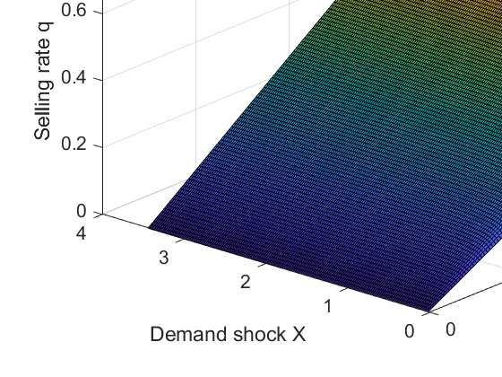
 Electronic copy available at: https://ssrn.com/abstract=3780858

• Daily mempool transaction count in Bitcoin from Apr 2016 to Sep 2020 (see Fig. 4).

Here = 1, 1 = 72, and 2 = 36 correspond to Jan 2013, Sep 2020, and Dec 2015, respectively.
It is worthwhile pointing out that the monthly aggregate inventory data, which is not directly
observable, is obtained by Athey et al. (2016) and available only from Jan 2013 to Dec 2015.
 The bitcoin price is informative to the set of parameters Θ1 = { , , H , L } in (3), while
the average fee rate , average block size Λ , and aggregate inventory are informative to the
set of parameters Θ2 = { , H , L , , }. Calibrating the parameters in Θ2 will be elaborated on
in Section 4.2.
 Our model assumes two regimes in bitcoin transaction: high-active regime and low-active
regime. In the high-active regime, the transaction is very active, implying a large number of orders
submitted by users and high volatility in bitcoin price. In the low-active regime, the transaction
of bitcoin is relatively less active, implying a small number of users’ orders and low volatility in
bitcoin price. Using the time series of the mempool transaction count,17 as shown in Fig. 4, we can
quickly identify two regimes. Indeed, one can observe that from the end of 2016 to the beginning
of 2018, the moving average of the mempool transaction count is much higher than that in the rest
periods. Then, we roughly divide the period of 2013 to 2020 into three parts:

 • low-active regime from 2013 to 2016 Q3,

 • high-active regime from 2016 Q4 to 2017 Q4, and

 • low-active regime from 2018 Q1 to 2020 Q3.

 Next, we set values for some parameters. We take the discount factor = 6% that is commonly
used in many empirical studies. We normalize the number of bitcoin to be one, i.e., ¯ = 1. The
 1
corresponding block rewards function becomes = 2 [ /4]+3
 as the block rewards halve every four
years. For computational simplicity, we assume that the Bitcoin block rewards will terminate in
 17Mempool is the set of all unconfirmed transactions from users in the Bitcoin network The mempool transaction
count refers to the total number of unconfirmed transactions in the mempool, The mempool transaction count data,
available at www.blockchain.com, is a good proxy for the number of unconfirmed transactions and is employed to
detect the high-active and low-active regimes. A high (low) mempool transaction count suggests a large (small) number
of unconfirmed transactions.

 17

 Electronic copy available at: https://ssrn.com/abstract=3780858

Figure 4: The high-active and low-active markets suggested by daily mempool transaction
count (in thousand) from 2016 to 2020. The red line represents the 60-day moving average.

2050, after which block rewards will be tiny and can then be neglected. The capacity of blocks
per unit of time is chosen as = 10. In fact, the average volume per transaction order since
2016 is around 1.05 bitcoin. Note that each block can accommodate about 4000 transaction
orders. This suggests that the capacity of number of orders that the Bitcoin system can process
in a year is 4000 × 6 × 24 × 365 = 210, 240, 000. Then the normalized capacity per year is
 = 1.05 × 210, 240, 000/21, 000, 000 ≈ 10, where 21, 000, 000 is the total actual number of
bitcoin. We set = 100, which implies that one unit change of the demand could lead to a change
of 100 billion USD in the bitcoin price. In fact, plays a role in scaling the demand factor , so
the value of does not affect our findings. We will choose = 0, as Athey et al. (2016) show that
the bitcoin velocity is approximately constant. For the parameters in the Beta distribution in (3.4),
we set ( 1 , 2 ) = (0.1, 99.9) and ¯ = 10%, which can capture the effect that the average fee rate
could increase dozens of times as the bitcoin price changes (see Fig. 2).
 We set the transition intensities H = 0.8 and L = 0.3, which implies an average duration of
1.25 years for the high-active regime and of 3.33 years for the low-active regime. The durations are
consistent with what we observe from the dynamics of the mempool transaction count. Furthermore,
we adopt the jump parameters = 57 and = 0.9 estimated by Gronwald (2015), which implies

 18

 Electronic copy available at: https://ssrn.com/abstract=3780858

a rough 10% downward jump once a week.
 We now use the bitcoin price to estimate the parameters Θ1 = { , , H , L } for the Gompertz
diffusion model of demand shock (i.e., Gutierrez et al., 2004). Based on the characterization of
high-active and low-active regimes from 2016 to 2020, we estimate the annualized volatility for
both high-active and low-active regimes and obtain H = 0.7910 and L = 0.6225, which suggests
that the demand shock in the high-active regime is more volatile than in the low-active regime.
Using the historical bitcoin prices and (2), we obtain the estimated values of Bitcoin’s adoption
speed and the log carrying capacity, i.e., = 1.2397 and = 0.6527.

4.2 Calibration method for Θ2 = { , H , L , , }

It remains to estimate the parameters Θ2 = { , H , L , , } by matching model outputs with the
observed data. We will calibrate Θ2 using the market data {( , ), = 1, 2, · · · } as well as the
observed bitcoin prices.
 With the observed bitcoin prices, we can recover the demand shock path over time { 
 e ; =

1, · · · , 1 } through Equation (2). Let { ; = 1, · · · , 1 } be the observed market states as given by
Fig. 4. Given the observed inventory level 
 e and demand level 
 e at time , we have

 = ( 
 e e , ; ),
 e , (20)

 e = ∗ ( e
 ), (21)

 e = ∗ ( , e ; Θ2 ),
 e , (22)

where (·, ·, ·; ) and ∗ (·) are as given in (7) and (10), respectively, and ∗ (·, ·, ·; Θ2 ), ∈ {H, L}
is the optimal selling rate given in (19) with a given set of parameters Θ2 and can be obtained
by numerically solving the HJB equation. We then obtain the following average fee rate {e
 , =
1, · · · , 1 }, average block size {Λ
 e , = 1, · · · , 1 }, and inventory { 
 e , = 2, · · · , 1 } implied by

 19

 Electronic copy available at: https://ssrn.com/abstract=3780858

the model:

 ( e )
 (Θ2 ) =
 e , (23)
 ( e )
 e (Θ2 ) = e
 Λ / 1{e 

Table 1: Summary of parameters.

 Parameters Symbol Value
 Discount rate 6%
 Total supply of bitcoin ¯ 1
 Capacity of blocks per unit of time G 10
 Hash rate per miner (TH/s) 5.2
 Coefficient in quantity equation (Billion USD per unit) 100
 Elasticity of bitcoin velocity to supply 0
 Upper bound of fee rate ¯ 10%
 Beta distribution parameters ( 1 , 2 ) (0.1, 99.9)

 Adoption speed of Bitcoin 1.2379
 Log carrying capacity 0.6527
 Volatility of demand shock in high-active regime H 0.7910
 Volatility of demand shock in low-active regime L 0.6225
 State transition intensity ( H , L ) (0.8, 0.3)
 Jump parameters ( , ) (57, 0.9)

 Parameter in liquidation cost 0.39
 Sensitivity of volume to demand in high-active regime H 346.5
 Sensitivity of volume to demand in low-active regime L 62.3
 Shape parameters in ( , ) (0.6, 8)

line) matches the observed one (the dashed line) well from 2013 to 2015. As shown by the dotted
line in the figure, the bitcoin price experienced a drastic increase and a gradual decline during
this period. This suggests that our model can capture the pattern that miners kept reducing their
bitcoin holdings regardless of bitcoin price’s drastic fluctuation. The pattern may be attributed to
three reasons. First, miners reduce their inventory to make profits and sustain their mining service.
Second, as will be shown in Section 5, we find that high jump risk is one of the major forces driving
miners to sell their bitcoin holdings at an early stage even when bitcoin prices are relatively low
or very volatile (see Fig. 8). Third, we find that transaction fees are another driving force for
miners to reduce their inventory. The intuition is quite simple. As users attach transaction fees, the
users’ bitcoin holding significantly affects the magnitude of transaction fees: the less the miners’
inventory, the larger the users’ bitcoin holding, and thus the higher the transaction fees (see also
Fig. 10). Moreover, as transaction fees will be the miners’ unique income source in the long-run,
miners have a strong incentive to reduce their inventory in order to make their mining business

 21

 Electronic copy available at: https://ssrn.com/abstract=3780858

sustainable.

 40 1200
 Implied miners‘ inventory
 Observed miners‘ inventory
 35 Bitcoin price (monthly, right) 1000

 In percentage (%) 30 800

 In USD
 25 600

 20 400

 15 200

 10 0
 2013 2014 2015

Figure 5: Implied miner’s proportional inventory from 2013 to 2015. The dashed black line
shows the observed miners’ proportional inventory based on the estimation from Athey et al. (2016).

 In panel A of Fig. 6, we plot the model-implied average fee rate (solid line), which captures
the features of the observed data (dashed line): 1) From 2014 to middle 2016, the average fee rate
was almost flat; 2) From late 2016 to 2018, the average fee rate rose dramatically. As shown in the
panel B of Fig. 6, the model-implied block size (solid line) well matches the observed data (dashed
line): 1) In the period 2013-2016, the block size was increasing but lower than 1MB, the block
capacity. 2) Since 2017, the blocks were almost full.18
 Combined with Fig. 6 and Proposition 1, our model can explain the co-movement of the block
size and the average fee rate. When Bitcoin demand is low (e.g., 2014-2016), blocks are not full and
the miners process all unconfirmed transactions. Then the average fee rate tends to be flat. When
the demand is so high (e.g., after 2017) that the volume of unconfirmed transactions significantly
exceeds the block capacity, miners should prioritize the validation of unconfirmed transactions with
higher fees. Thus, blocks could be almost full and the average fee rate may increase dramatically.19
 18Before 2019, the largest capacity for a block was 1MB. Since 2019, the block capacity increased slightly as a new
process SegWit was introduced in Bitcoin system; see https://en.wikipedia.org/wiki/SegWit.
 19There are some slight mismatches between model-implied results and observed data. They may be partially due
to the irrational behaviors in Bitcoin mining in an early period (e.g., 2013) and imperfect identification of regimes in
Bitcoin transactions.

 22

 Electronic copy available at: https://ssrn.com/abstract=3780858

A. Average Fee Rate B. Average block size
 0.35 1.4
 Implied average fee rate Implied average block size
 Observed market average fee rate Observed average block size
 0.3 1.2

 0.25 1

 In Megabytes (MB)
 In percentage (%)

 0.2 0.8

 0.15 0.6

 0.1 0.4

 0.05 0.2

 0 0
 2013 2014 2015 2016 2017 2018 2019 2020 2013 2014 2015 2016 2017 2018 2019 2020

Figure 6: Implied average fee rate and implied average block size from 2013 to 2020. The
dashed line in panel A represents the monthly observed average fee rate.The dashed line in panel B
represents the monthly observed average block size.

5 Quantitative Analysis

We shall conduct an quantitative analysis in this section with the parameter values of Table 1 as
default values.

5.1 The miner’s optimal strategy

 A. Short-run case B. Long-run case
 1.6 1.8
 J
 =0 J
 =0
 1.5 1.7

 1.4 1.6

 1.3 Selling Region 1.5 Selling Region
 Demand shock X

 Demand shock X

 1.2 1.4

 1.1 1.3

 1 1.2

 0.9 1.1

 0.8 Holding Region 1 Holding Region
 0.7 0.9

 0.6 0.8
 0 0.1 0.2 0.3 0.4 0.5 0 0.1 0.2 0.3 0.4 0.5 0.6 0.7 0.8 0.9 1
 Inventory Ht Inventory Ht

Figure 7: Selling and holding regions in the high-active regime with no jump risk ( = 0).
Parameter values are based on Table 1. The left panel shows the short-run case, i.e., with block
rewards, = 2014 and = 0.5871. The right panel shows the long-run case in which the block
rewards are terminated, i.e., = 2140.

 23

 Electronic copy available at: https://ssrn.com/abstract=3780858

Optimal selling barrier, selling region, and holding region. Fig. 7 shows the miner’s
liquidating strategies for the short-run case ( = 2014, the left panel) and the long-run case (the
right panel), where the high-active regime with no jump risk ( = 0) is assumed, the cumulative
supply of bitcoin is = 0.5871 for the short-run case, and other default parameters are reported
in Table 1. Numerical results for the low-active regime are quite similar and are thus omitted here.
It shows that there exists an optimal selling barrier, splitting the solution region into a holding
region and a selling region in which the miner holds and sells her inventory, respectively. For a
fixed inventory level, the selling region is below the (optimal) selling barrier because the miner is
inclined to reduce her inventory when the demand shock is lower enough.
 It can be observed from Fig. 7 that the selling barrier decreases as the inventory level increases
partially because a higher inventory prompts miners to reduce their inventory earlier in order to
receive higher transaction fees in the future. Note that the selling barrier slightly decreases with
inventory in the short-run case (the left panel of Fig. 7), as block rewards significantly prevail over
the transaction fee income in this case. As shown by the right panel of Fig. 7 for the long-run case,
the selling barrier exhibits a clear downtrend against inventory. This is because in the long run,
transaction fees are the unique source of miners’ income, and miners are inclined to reduce their
inventory to increase potential transaction fee income.
 Jump risk or high volatility? The jump intensity and the volatility H ( L ) impact the
miner’s optimal selling strategy quite differently. In particular, we shall point out a reasonably high
volatility cannot explain why miners kept selling their inventory in 2014-2015..
 Fig. 8 plots the selling barrier against jump intensity for the short-run case ( = 2014),
where the high-active regime is assumed, = 0.5871, / = 0.1, and other default parameter
values are given in Table 1. As jump intensity increases from 0 to 57, the selling barrier decreases
from around 1.6 to 0. This implies that jump risk could hasten miners’ selling of bitcoin holdings.
In particular, for a high jump risk, e.g., = 57, miners keep selling their bitcoin holdings. We
then infer that the jump risk is a primary factor determining miners’ optimal selling timing. This
also explains why miners started to sell their holdings to market at the inception of Bitcoin even

 24

 Electronic copy available at: https://ssrn.com/abstract=3780858

A. Selling barrier v.s. J B. Selling barrier v.s.
 1.4 1.8

 1.6
 1.2

 1.4
 1
 1.2
 Selling barrier

 Selling barrier
 0.8
 1

 0.6 0.8

 0.6
 0.4
 0.4
 0.2
 0.2

 0 0
 0 10 20 30 40 50 60 100 120 140 160 180 200 220 240 260 280 300
 J Volatility (%)

Figure 8: Impact of jump intensity and volatility H ( L ) on the selling barrier for the
short-run case in the high-active regime. Parameter values are based on Table 1. For panel B,
we assume H = L = varying from 100% to 300%. We choose = 2014 and / = 0.1 with
 = 0.5871.

when bitcoin prices and demands were extremely low. Note that the demand level implied from
bitcoin price could be as low as 0.073 in 2014-2015 and increased to 4.03 in 2017. In contrast, a
reasonably high volatility in Bitcoin demand shock could not drive miners to sell when the bitcoin
demand was so low in 2014-2015. For example, as shown in the right panel of Fig. 8, even for the
volatility of 300%,20 the selling barrier is higher than 0.2, which is much higher than the demand
level 0.073 in 2014-2015. Therefore, a reasonably high volatility cannot explain why miners kept
selling their inventory in 2014-2015.
 Optimal selling rate. Fig. 9 depicts the miner’s optimal selling rate against demand shock and
inventory level for the short-run case ( = 2014) in a high-active regime with no jump risk ( = 0).
The optimal selling rate appears to be smooth and non-decreasing with respect to both inventory
and demand levels.
 20Note that Liu and Tsyvinski (2018) estimate the bitcoin price volatility with daily, weekly, and monthly data and
find the annualized volatility varies from 106.03% to 240.61%.

 25

 Electronic copy available at: https://ssrn.com/abstract=3780858

Figure 9: Optimal selling rate against demand shock and inventory for the short-run case in
the high-active regime with no jump risk = 0. Here = 2014 with = 0.5871, and other
default parameter values are as given in Table 1.

5.2 Average transaction fee rate

Now let us investigate the properties of the average transaction fee rate. Fig. 10 plots the miner’s
average transaction fee rate against the demand shock in the high-active regime (panel A) and the
low-active regime (panel B), respectively. It can be seen that consistent with Proposition 1, the
average transaction fee rate in both the long-run case (solid lines) and the short-run case (dashed
lines) is non-decreasing in demand shock, as a higher demand shock results in a larger volume
of unconfirmed transactions. Moreover, as predicted by part (i) of Proposition 1, the average
transaction fee rate is likely flat when the demand shock is sufficiently low. One can also observe
that the average fee rate in the long-run is always no lower than in the short-run, which is not
surprising because, ceteris paribus, there are more circulated bitcoins and thus more transactions
in the long-run than in the short-run. In addition, the average fee rate in the low-active regime is
lower than or equal to that in the high-active regime, as more transactions occur in the high-active
regime.

 26

 Electronic copy available at: https://ssrn.com/abstract=3780858

10-3 A. High-active market 10-3 B. Low-active market
 2.5 2.5
 Long-run: H t =0.2 Long-run: H t=0.2
 Long-run: H t =0 Long-run: H t=0

 2 Short-run: Ht =0.2 2 Short-run: H t=0.2
 Average transaction fee rate

 Short-run: Ht =0 Short-run: H t=0

 1.5 1.5

 1 1

 0.5 0.5

 0 0
 0 0.5 1 1.5 2 2.5 3 0 0.5 1 1.5 2 2.5 3
 Demand shock x Demand shock x

Figure 10: The average fee rate against demand shock for different inventory. The short-run
case is at = 2014. The left panel is for the high-active regime, while the right panel is for the
low-active regime.

 We further examine how the miner’s holding affects transaction fees. As shown in Fig. 10,
the average fee rate with = 0.2 (black lines) is always lower than that with = 0 (gray lines).
Intuitively, ceteris paribus, the more bitcoins held by miners, the fewer bitcoins held by users, and
the fewer users’ unconfirmed transactions as a result. Combined with Proposition 1, this explains
why a higher miner’s inventory could induce a lower average fee rate.

5.3 The miner’s value function

We now examine how transaction fees and the declining block rewards affect the miner’s value in
Bitcoin mining in both short run (with block rewards) and in long run (without block rewards). For
computational simplicity, the block rewards are assumed to terminate in 2050, as there are very few
block rewards from 2050 and ultimately no block rewards from 2140. Fig.11 presents the miner’s
value against time without (solid line) and with jump risk (dashed line), respectively. The dashed
line is always below the solid line because jump risk hurts the miner’s value.
 Note that in both cases, the miner’s value against time is U-shaped, which can be attributed to
the declining block rewards and endogenous Bitcoin transaction fees. Indeed, at the early stage of
the Bitcoin system when the transaction volume is low while block rewards are high, the majority of

 27

 Electronic copy available at: https://ssrn.com/abstract=3780858

a miner’s income comes from block rewards. As such, the declining block rewards predetermined
by the system lead the miner’s value to be decreasing with time at the early stage, ceteris paribus.
As time goes up, endogenous transaction fees would eventually dominate the miner’s value, even
before the termination of block rewards, which explains the increasing part of the miner’s value.

 300
 J
 =0

 J
 =10
 250
 Miner value (in billion US dollars)

 200

 150 High reward+low fees

 100
 Low reward+high fees

 50

 0
 2010 2015 2020 2025 2030 2035 2040 2045 2050 2055 2060

Figure 11: The miner’s value function across time in the high active regime. Here the initial
demand = 1 and initial inventory 0. Note that in the beginning the block rewards are high but
the endogeneuous transaction fees are low, while in the long run the block rewards diminish but the
endogenous transaction fees become high.

6 Conclusion

We develop a continuous-time dynamic model to study the economics of the supply side of bitcoin
mining, inspired by the classic Hotelling model for exhaustible resources. The model is rich enough
to incorporate endogenous transaction fees, the miners’ liquidation policies, endogenous inventory
holdings, declining system block rewards, and stochastic demand. We find that high jump risk
and transaction fees are major forces driving miners to reduce their inventory even when bitcoin
prices are extremely low, consistent with empirical observations. The model gives an explanation
for the observed co-movements of average transaction fee rate, average block sizes, and Bitcoin
prices, especially why the average transaction fee rate stays flat from 2014 to 2016 and increases
dramatically in 2017.

 28

 Electronic copy available at: https://ssrn.com/abstract=3780858

References

Alsabah, H. and Capponi, A. 2019. Pitfalls of Bitcoin’s Proof-of-Work: R and D Arms Race and
 Mining Centralization. mimeo Columbia University.

Athey, S., Parashkevov, I., Sarukkai, V., and Xia, J. 2016. Bitcoin pricing, adoption, and usage:
 Theory and evidence. Working paper.

Bass, M. F. 1969. A new product growth for model consumer durables. Management Science 15
 215-227.

Bass, M.F. 2004. Comments on "A new product growth for model consumer durables": the Bass
 model. Management Science 50 1833-1840.

Basu, S., Easley, D., O’Hara, M., and Sirer, E. G. 2018. Towards a Functional Fee Market for
 Cryptocurrencies. Working paper.

Ben-Or, M. (1983). Another advantage of free choice: completely asynchronous agreement proto-
 cols. Proceedings of ACM PODC 1983.

Benigno, P., Schilling, L., and Uhlig, H. 2019. Cryptocurrencies, Currency Competition, and the
 Impossible Trinity. Working paper.

Biais, B., Bisière, C., Bouvard, M., Casamatta, C., and Menkveld, A. 2018. Equilibrium Bitcoin
 pricing. TSEWorking Paper.

Biais, B., Bisière, C., Bouvard, M., and Casamatta, C. 2019. The Blockchain Folk Theorem. Review
 of Financial Studies 32 1662-1715.

Bohme, R., Christin, N., Edelman, B., and Moore, T. 2015. Bitcoin: Economics, Technology, and
 Governance. Journal of Economic Perspectives 29 213-238.

Bolt, W. and Oordt, M. 2016. On the value of virtual currencies. Working Paper.

 29

 Electronic copy available at: https://ssrn.com/abstract=3780858

Catalini, C. and Gans, J.S. 2016. Some simple economics of the blockchain, National Bureau of
 Economic Research Technical report.

Chaum, D. (1983). Blind signatures for untraceable payments. Working Paper.

Chiu, J. and Koeppl, T. 2017. The economics of cryptocurrencies-Bitcoin and beyond. Working
 paper.

Cong, L., He, Z., and Li, J. 2018. Decentralized mining in centralized pools. Forthcoming at Review
 of Financial Studies.

Cong, L., Li, Y., and Wang, N. 2019. Tokenomics: Dynamic Adoption and Valuation. Forthcoming
 at Review of Financial Studies.

Detzel, A., Liu, H., Strauss, J., Zhou, G., and Zhu, Y. 2018. Bitcoin: Learning and Predictability
 via Technical Analysis. Working paper.

Dixon, R. 1980. Hybrid Corn Revisited. Econometrica 48 1441-1451.

Cuoco, D. and Liu, H. 2000. Optimal consumption of a divisible durable good. Journal of Economic
 Dynamics and Control. 24 561-613.

Dwork, C. and Naor, M. 1992. Pricing via processing or combating junk email. Proceedings of
 CRYPTO 1992, 139-147.

Easley, D., O’Hara, M., and Basu, S. 2019. From mining to markets: the evolution of transaction
 fees. forthcoming in Journal of Financial Economics.

Fischer, M. J., Lynch, N. A. and Paterson, M. S. 1985. Impossibility of Distributed Consensus with
 One Faulty Process. Journal of the ACM. 32 374–382.

Gronwald, Marc. 2015. The Economics of Bitcoin-News, supply vs. Demand nd Jumps. Working
 paper.

 30

 Electronic copy available at: https://ssrn.com/abstract=3780858