Employment Effects of Unemployment Insurance Generosity During the Pandemic
←
→
Page content transcription
If your browser does not render page correctly, please read the page content below
Munich Personal RePEc Archive

Employment Effects of Unemployment
Insurance Generosity During the
Pandemic

Scott, Dana and Finamor, Lucas

Yale University

12 August 2020

Online at https://mpra.ub.uni-muenchen.de/102390/
MPRA Paper No. 102390, posted 13 Aug 2020 07:58 UTC
Employment Effects of Unemployment Insurance Generosity
                        During the Pandemic∗

                                        Lucas Finamor†                    Dana Scott‡
                                                  First Draft: July 14, 2020
                                                 This Draft: August 12, 2020

                                                           Abstract
           In response to the Covid-19 pandemic, the United States enacted the CARES Act, which expanded
       unemployment insurance (UI) benefits by providing a $600 weekly payment in addition to state un-
       employment benefits. We test whether changes in UI benefit generosity are associated with decreased
       employment, both at the onset of the benefits expansion and as businesses began to reopen. We use data
       from Homebase, a private firm that provides scheduling and time clock software to small businesses,
       which allows us to exploit high-frequency observations to understand how firms and workers respond
       to policy changes in real time. While our results show that relative declines in employment and hours
       occurred in mid-March, we find that the workers with higher post-CARES replacement rates did not
       experience larger declines in employment or hours of work when the benefits expansion went into effect.
       They have also returned to their previous jobs over time at similar rates as others.

    Keywords: Unemployment Insurance, Employment, COVID-19, CARES Act

    JEL Codes: J65, J68

   ∗ We are very grateful to Homebase for making the data available for this research and thank Ray Sandza and Andrew Vogeley at

Homebase for assisting us in understanding the data. This paper builds upon the July 14th draft, which was co-authored with Joseph
Altonji, Zara Contractor, Ryan Haygood, Ilse Lindenlaub, Costas Meghir, Cormac O’Dea, Liana Wang, and Ebonya Washington.
We would like to thank Eduardo Ferraz for comments. We are also grateful to the Cowles Foundation and the Tobin Center for
Economic Policy at Yale University for funding. Mistakes and opinions are our responsibility.
   † Yale University - Department of Economics, lucas.finamor@yale.edu
   ‡ Corresponding Author. Yale University - Department of Economics, 28 Hillhouse Avenue, New Haven, CT 06511,

dana.scott@yale.edu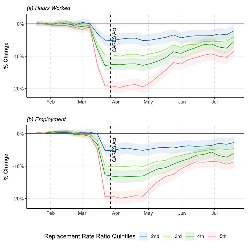
1 Introduction

The Coronavirus Aid, Relief, and Economic Stimulus (CARES) Act instituted a variety of economic policy

responses to the Covid-19 pandemic in the United States. One such policy was a large, temporary expansion

of unemployment insurance (UI) benefits known as Federal Pandemic Unemployment Compensation. The

expansion provided a $600 weekly payment in addition to any state unemployment benefits for which a

worker would have already been eligible.

   The payment was designed to replace 100 percent of the mean U.S. wage when combined with existing

UI benefits. However, the extra $600 weekly payment provided under CARES yields a total UI benefit that

is greater than weekly earnings when working for the median worker. Ganong et al. (2020) estimate ex post

replacement rates over 100 percent for 68 percent of unemployed workers who are eligible for UI, as well as

a median replacement rate of 134 percent. Given the moral hazard effects of unemployment benefits that are

well-established in the literature, it is natural to ask whether such high replacement rates affect employment

levels under the distinct conditions of the pandemic.1

   In this paper, we test whether higher UI benefits are associated with decreased employment, both at the

onset of the benefits expansion and as businesses reopened. We use data from Homebase, a private firm that

provides scheduling and time clock software to small businesses, which allows us to exploit high-frequency

observations to understand how firms and workers respond to policy changes in real time. The longitudinal

data allows us to estimate UI benefits for each worker in our sample and to follow their labor market status

through early 2020. Our sample over-represents small businesses with hourly workers. This population is

of particular interest for our study, because they were disproportionately affected by the pandemic (Bartik

et al., 2020a) and face higher replacement rates after CARES, given their lower earnings.

   First, we employ an event study design to test whether exposure to higher replacement rates after the

passage of the CARES Act on March 27 is associated with a differential decrease in employment or hours of

work. We complement these results with a parsimonious specification testing directly for incremental effects

after the benefits expansion. In both analyses, we flexibly control for state-industry-week trends. We find

that workers with more generous UI benefits did not experience differential declines in employment after the

CARES Act was passed. While there is a negative association between replacement rates and employment,

it is fully established before March 27. Our study benefits from high-frequency data that allows us to isolate
  1 Schmieder   and von Wachter (2016) review the literature on moral hazard effects of unemployment insurance.

                                                               1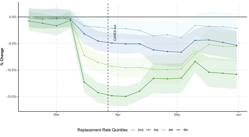
the timing of the CARES Act from other drivers of reduced employment beginning in mid-March. Such

factors include the pandemic-induced decline in labor demand, fear and concern about public health, and

increased childcare costs.

    We support our main results with several robustness exercises varying the dates of analysis, the defini-

tions of treatment and outcome variables, and the set of controls. We also test whether exposure to higher

replacement rates makes workers less likely to return to work, conditional on working at firms with ob-

servably increasing labor demand. Additionally, we test whether workers’ wages increase when they are

re-hired. Acknowledging the limitations of our data and sample restrictions, we conduct additional exer-

cises on a broader sample of workers in the Homebase data by exploiting variation in state-industry median

replacement rates. We also replicate our main results using the Current Population Survey (CPS). All of the

additional tests support the same conclusion: the negative labor market effects associated with replacement

rates are attributable to changes in mid-March; we do not observe negative effects after the passage of the

CARES Act. If anything, groups facing larger increases in benefit generosity experience slight gains in

employment relative to the least-treated group starting in early May. Furthermore, the CPS exercise high-

lights that our results are not merely an artifact of our sample selection or of the structure of our analyses.

Rather, they are representative of trends in the labor market more broadly. These results suggest that, in

the aggregate, the expansion in benefit generosity did not decrease employment at the outset, and that high

replacement rates did not make workers differentially less likely to return to work.

    It is important to emphasize the limitations of our study. First, our empirical strategy is not suitable

to estimate the causal effect of replacement rates and should not be interpreted as such. We can, however,

test the differential responses before and after the CARES Act. Second, the Homebase data over-represents

small businesses and is concentrated in specific sectors, e.g. restaurants. Third, in order to precisely estimate

workers’ replacement rates we restrict our sample to workers with relatively high attachment to their jobs.

Fourth, since our analyses rely on links between firms and workers within the Homebase universe, we cannot

observe rehiring activity outside of Homebase firms.

    Our analysis contributes to the growing literature on labor market effects of Covid-19. Our findings are

consistent with other results in the literature: lower-wage workers, who have higher ex post replacement

rates, were the most affected in the early weeks of the pandemic. Goolsbee and Syverson (2020) highlight

the role of agents’ fear and individual choices to stay home in determining economic activity during the

pandemic. Altonji et al. (2020), Bartik et al. (2020a), Cajner et al. (2020), Chetty et al. (2020), Fairlie

                                                       2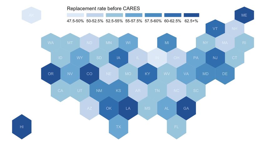
et al. (2020), Gupta et al. (2020), and Montenovo et al. (2020) use various data sources – including the

Homebase data – to document trends in employment and spending during the pandemic. Ganong et al.

(2020) estimate ex post replacement rates over 100 percent for 68 percent of unemployed workers who are

eligible for UI, as well as a median replacement rate of 134 percent. Bartik et al. (2020a) use data from

Homebase to show that states with higher ex post median replacement rates tended to have lower initial

decreases in employment and recovered more quickly than others with lower replacement rates. Marinescu

et al. (2020) use job application and vacancy data to assess whether increasing replacement rates under the

CARES Act cause employers to have difficulty rehiring workers. They find that while applications and

applications-per-vacancy decreased more for occupations and states with larger increases in the replacement

rate, these differences are not explained by the CARES Act alone. These results are consistent with our

findings. We contribute to this literature by leveraging high-frequency data linking individuals and firms

to directly estimate workers’ replacement rates and observe individual employment, hours of work, and

re-hiring over time.

    Many works analyze the effects of increasing unemployment benefits during recessions, including Mit-

man and Rabinovich (2015), Hagedorn et al. (2016), Landais et al. (2018), and Hagedorn et al. (2019), who

explore the UI duration extension during the Great Recession. The policy change that we analyze provides

an advantage: the extra generosity was the same across all states and was not endogenously determined

by local economic conditions. Nevertheless, we emphasize that the Covid-19 pandemic presents a unique

context – combining a health and an economic crisis – from which it is difficult to generalize labor market

effects of UI. First, median replacement rates are over 100 percent for the first time in the United States.

Workers may behave much differently when facing current replacement rates than they would under ordinary

circumstances. Second, the public health context makes the current moment distinct from other recessions

because it creates unique barriers to labor force participation, such as the fear effect documented in Goolsbee

and Syverson (2020), safety concerns associated with working, and increased costs of childcare.

    The paper proceeds as follows. In the next section we present the institutional setting of unemployment

benefits in the United States and changes under the CARES Act. We present the data and sample restrictions

in Section 3 and the empirical strategy in Section 4. Section 5 provides the main results. We conduct

additional exercises in Section 6.

                                                      3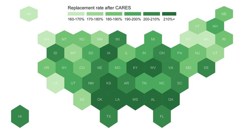
2 Institutional background

2.1     UI benefits eligibility

To compute an individual’s eligibility for unemployment benefits, all states use a worker’s earnings in the

four most recent completed quarters. Most compute benefits as a percentage of the worker’s highest quarterly

earnings, second-highest quarterly earnings, or annual earnings, subject to a minimum and maximum benefit

level (Ganong et al., 2020). The generosity of benefits varies substantially by state, as shown in Appendix

Figure A.2. To compute UI benefits, we use workers’ earnings histories in the four quarters of 2019.

      While the CARES Act expanded eligibility for UI, several institutional features restricting eligibility

remain. First, even under CARES, a worker who quits her job is ineligible for UI. While workers who quit

due to exceptional circumstances related to Covid-19 – e.g. having a respiratory condition that makes work

risky – are exempted from this, those who quit for no reason other than concern about contracting Covid-19

are not eligible for UI. Second, once a person receives a “suitable offer of employment,” they are no longer

eligible for UI even if they reject the offer. The Department of Labor states that “a request that a furloughed

employee return to his or her job very likely constitutes an offer of suitable employment that the employee

must accept” (U.S. Department of Labor (2020)). In practice, compliance with both rules may be lower at

small firms where employers interact with workers more informally.

2.2     Timing of the CARES Act

On Thursday, March 19, Senate Republicans introduced a $1 trillion economic relief package. The bill in

its original form did not include supplemental unemployment insurance (Sullivan (19 March 2020)). News

coverage of the progress of the bill indicates that legislators agreed to include supplemental unemployment

benefits on Monday, March 22 (Cochrane et al. (22 March 2020)). The structure of unemployment benefits

continued to be contested throughout the week, particularly the duration of the benefits extension. The bill

passed the Senate on March 25 and the House of Representatives on March 26, and was signed into law on

Friday, March 27.

      The timing of events in the passage of the stimulus bill is relevant to employers’ and workers’ plausible

responses to the policy intervention. Since supplemental unemployment insurance did not appear in the draft

bill until Monday of the week in which it was passed, and was contested in subsequent days, it is unlikely

that the decision to open a firm in the week beginning March 21 or to lay off a worker prior to the start of

                                                       4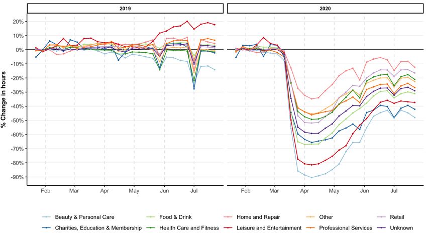
work in that week could have been influenced by anticipation of enhanced unemployment benefits.

3 Data

Our main dataset comes from Homebase, a private firm that provides scheduling and time clock software

to small businesses, covering a sample of hundreds of thousands of workers across the U.S. and Canada.

Homebase’s clients are primarily small firms that require time clocks for their day-to-day operations, nearly

half of which are in the food and drink industry. The basic version of Homebase is free to firms. Workers

are predominantly hourly, not salaried, employees.2

    Because of these limitations, insights about the Homebase sample are not representative of the entire

labor market. However, as Bartik et al. (2020a) note, the population covered by Homebase is of particular

policy interest since it represents a segment of the labor market disproportionately affected by the pandemic.

In the context of unemployment benefits generosity, the Homebase sample is valuable because it covers

workers with relatively low wages: most are in the first and second quintiles of national earnings from the

CPS (Altonji et al., 2020). These workers thus experience particularly high UI replacement rates from the

addition of the $600 supplemental payment.

    We use the data’s longitudinal structure to follow workers and firms over time, beginning in 2018. We

observe workers’ daily shift data, including hours worked, hourly wage, and total earnings.3 Each worker is

linked to a firm. For each firm, we observe state, metro area, and industry.4 We impose the following data

restrictions: i) we keep firms that logged positive hours for at least 5 weeks between 2019-2020, ii) we keep

workers who worked at least 20 hours per week in the baseline period (January 19 to February 8, 2020), and

iii) we keep only workers who were employed in all quarters of 2019, with positive earnings and at least 300

hours worked in each quarter.

    The last requirement is the most restrictive. We impose it because we need to observe a worker’s 2019

earnings history to accurately compute their unemployment benefits. Since we only observe an individual’s

work history when their firm is in the Homebase data, this restriction aims to exclude individuals who

worked in other jobs during 2019.5 We compute pre- and post-CARES UI benefit replacement rates using
   2 While some firms could also list their salaried employees in the data, their earnings are not usually recorded. We thus exclude

them from our analysis.
   3 Wages and earnings are available for approximately 52% of the workers. This variation is determined at the firm level, since

some firms use the software just to register shifts but not to track payroll.
   4 We show industry composition in table A.1.
   5 Some workers in Homebase may have worked for other firms, either full-time prior to their employment at the Homebase

                                                                 5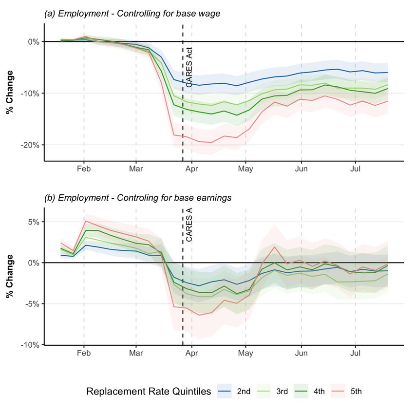
the calculator developed by Ganong et al. (2020) using state identifiers and earnings in the four quarters of

2019. When computing workers’ quarterly earnings, we floor their wages at the state minimum wage. Many

workers’ posted wages are below the state minimum because they work for tips. However, U.S. labor law

requires that employers must “top up” workers’ wages to the state minimum wage if their effective wage in

a given week is below the state minimum.

    The resulting dataset has 29,005 workers. We present descriptive statistics in table 1. In the base period,

which covers the three weeks between January 19 and February 8, these individuals worked on average

36.9 hours per week and earned an average hourly wage of $13.3, resulting in average weekly earnings of

$495.41, similar to average weekly earnings in 2019 of $479.50. Under state benefit schemes prior to the

CARES Act, the unemployment benefit levels in our sample result in replacement rates from 6.4% to 88.6%,

with a mean of 55.1%. After the CARES Act, replacement rates range from 27.3% to 410.8%, with a mean

of 192.4%. We group the sample into quintiles by post-CARES replacement rate. The range, mean, and

median of each quintile are presented in panel B of table 1.

    We note that the above restrictions necessarily exclude the shortest-tenured workers at a given firm,

as well as workers at newly established firms. Our sampled workers may be less likely to be laid off in

an economic downturn than shorter-tenured workers. In addition, the Homebase data is subject to some

additional limitations. Notably, workers who have been furloughed (i.e. are still employed by a firm but

are not working any hours) are not distinguishable from workers who have been formally laid off. In order

to overcome this limitation we code all workers that do not report hours for three days in a row as being

non-employed. This choice is likely to overestimate any effect of the policy on non-employment because

lower-earning workers have higher replacement rates and also are more likely to have irregular or reduced

work schedules during the pandemic. Thus they would be more likely to be erroneously coded as non-

employed.6 In the Appendix we also show that our conclusions are robust to more traditional labor market

data from the CPS. However, using this data imposes constraints on our analysis, since it does not allow

us to track workers’ employment and hours on a daily basis or to follow them for more than four months.

Particularly in the early weeks of the pandemic, the policy and public health situation changed rapidly, so

we lose granularity with lower-frequency data.
member firm or part-time concurrently with their employment at the Homebase member firm. Workers’ UI benefits are computed
on the basis of their total earnings in the last four quarters, so we drop workers for whom we are likely to not be observing their full
earnings history. Furthermore, if a worker has multiple jobs and is only laid off from the job at the Homebase member firm, they
would not be eligible for UI benefits.
   6 As discussed in section 5.2, the conclusions are robust to changes in this definition.

                                                                   6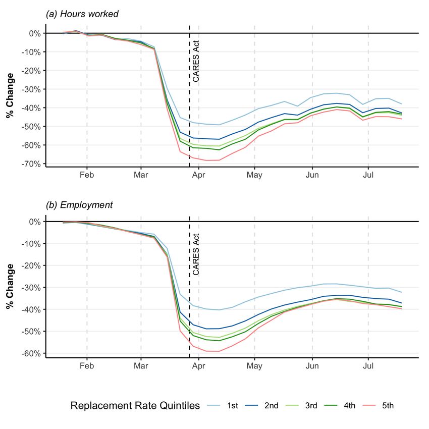
We supplement our dataset with two additional sources. To track start and end dates of state-level

restrictions in response to the pandemic, we use the COVID-19 US state policy database maintained by

Raifman et al. (2020). We use four types of restrictions: stay-at-home orders, closures of non-essential

businesses, restrictions on restaurants, and closures of gyms. Additionally, we use data on new Covid-19

cases from The New York Times to measure the pandemic’s severity across states.

4 Empirical approach

4.1      Measuring replacement rates

The ex post replacement rate Ri js for individual i working in industry j in state s is determined by her

pre-CARES UI benefits (UIiPre
                           js ), the additional $600, and her weekly earnings in a chosen reference period

(wi js ). In our baseline specification we choose wi js to be her average weekly wage in 2019. Formally:

                                                                UIiPre
                                                                    js + 600
                                                      Ri js =                   .                          (1)
                                                                       wi js

We also estimate our specifications with an alternative definition of the treatment variable. Since the ex post

replacement rate is mechanically related to the ex ante replacement rate, we test the robustness of our main

results to a specification in which we exploit variation from the differential change in replacement rates from

the incremental $600. We substitute the replacement rate with the replacement rate ratio Rratio
                                                                                          i js , formally:

                                                                UIiPre
                                                                    js +600
                                                 Ri js              wi js             600
                                          Rratio
                                           i js = Pre =                        = 1+          ,             (2)
                                                 Ri js            UIiPre
                                                                      js              UIiPre
                                                                                          js
                                                                  wi js

which measures the change in UI generosity. By construction, Rratio
                                                              i js is 1 for all workers pre-CARES. This

definition has the advantage of removing part of the mechanical effect of wages on the denominator of

equation 1 and of changing the direction of the effect of ex ante state generosity on the replacement rate

variable.7 While this measurement strategy does address some endogeneity concerns with respect to the

states’ ex ante replacement rates, it is not clear that Rratio
                                                         i js is the relevant price in workers’ labor supply

decisions.
  7 Ex   ante more-generous states have higher R but lower Rratio , holding wage constant.

                                                                   7
4.2 Event study
Leveraging the frequency of the data, we explore how workers facing different UI generosity post-CARES
behave before and after the benefits expansion. Our main analysis consists of two strategies. Our first
strategy looks into workers’ weekly employment status and hours worked over time depending on their ex
post replacement rate. We estimate the event study specification:
T 5
Yi jst = α0 + ∑ ∑ βtg Rgijs ✶{t = τ } + η jst + εi jst , (3)
τ =0 g=2
where Yi jst is the outcome for worker i associated with industry j in state s during week t. Rgijs is an indicator
that worker i’s replacement rate after the CARES Act places them in replacement rate quintile g. η jst is a
state-industry-week fixed effect, which subsumes all state-industry weekly variation, including the severity
of the pandemic in each state and states’ restrictions on business activities.
This strategy allows us to explore the labor market dynamics for individuals with different replacement
rate levels, before and after the CARES Act. We explore the differential treatment intensity, that is, the
generosity of UI measured in terms of the replacement rate, to empirically assess whether workers with
higher R have differential employment and hours of work trajectories.
While the first strategy allows us to investigate the full dynamics of the labor market outcomes, in the
second strategy, we combine the pre- and post-CARES coefficients to test directly if there were differen-
tial responses after CARES. With this parsimonious specification we leverage the frequency of the data,
estimating the following specification at the daily level:
Yi jsdt = α1 + γ Ri js + δ Postdt × Ri js + η jst + νd + εi1jsdt , (4)
where Ri js is the replacement rate, Postdt is an indicator for the period after the CARES Act, and νd a day-
of-the-week fixed effect. All other variables and parameters are the same as equation 3.8 We estimate this
specification in the window between March 15 and July 27. The initial date is chosen to define the pre-
period as the time when the economy had already been affected by the pandemic, but the CARES Act had
not yet passed. As in the first approach, we test if higher replacement rates are associated with differential
labor market outcomes after CARES. In both specifications, we cluster standard errors at the worker level
8 Panel (a) of table 2 shows results with the replacement rates in quintiles as in equation 3; panel (b) shows results using the
continuous replacement rate.
8following Bertrand et al. (2004) and Abadie et al. (2017).
Our strategies do not estimate a causal effect of the replacement rate on labor outcomes, as we do
not estimate a counterfactual path of labor outcomes without the benefits expansion. Instead, we explore
differences in the treatment intensity and assess empirically whether a relatively higher replacement rate is
associated with lower employment or hours after CARES. If that is true, δ will be negative in equation 4
and the βtg s will be declining in equation 3 after March 27.
The most important assumptions in our analysis are i) that individuals did not anticipate the decision
and exit the labor force before the Act was approved, and ii) there are no other factors that correlate with
R and are simultaneous to the CARES act. We argue that anticipation is unlikely for two reasons. First,
the timeline of negotiations indicates that the $600 additional benefit was not agreed upon until at least
Tuesday, March 24. Even if workers stopped working the following day, they would be coded as employed
in the entire pre-period. Second, workers will face any increased incentive to exit only after they are able to
receive extra benefits. Even though CARES became law on March 27, workers would not become eligible
for expanded benefits until the following week. Indeed, in many states, implementation took effect on a
much longer timeline and workers were not able to receive enhanced benefits for several more weeks. In
order to violate ii), a factor would need to correlate with labor market outcomes and R, within state-industry,
and have a differential effect before and after March 27th, such that the pre-CARES replacement rate would
not capture it.
5 Results
5.1 Event Study
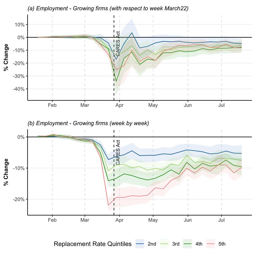
Figure 1 shows weekly trends for employment and hours of work for workers in our sample by replacement
rate quintile. Individuals with higher replacement rates had a larger reduction in hours of work and are
less likely to be employed relative to the baseline period (January 19 to February 8).9 However, it is clear
that both drops occurred in mid-March, before the CARES Act. Differential changes in labor outcomes are
concurrent with the beginning of the labor market shock of the pandemic, but not with the legislation. All
groups behave similarly after the Act took effect; we do not see any evidence of more negative results for
the higher quintiles.
9 An individual is coded as employed in a given week if she worked any positive hours in that week.
9In Appendix Figure A.1 we reproduce one graph from Altonji et al. (2020) to show that the drop occurred
at the same time – the two weeks of March prior to the passage of the CARES Act – for all industries and
that no similar trend is detected in 2019. From this figure is also clear that there is heterogeneity in the size
of the effect by industries which motivates our event study specification, where we control for state-industry
effects that vary over time.
Figure 2 plots the βtg coefficients on the interaction between the week dummies t and the replacement
rate quintiles g in equation 3 with 95% confidence intervals. The coefficients represent the percentage
change in hours (panel a) and probability of employment (panel b) relative to the first replacement rate
quintile in a given week. We control for state-industry-week effects in both panels.
The results are similar to the averages without controls shown in figure 1: workers with different UI gen-
erosity did not experience different declines in hours and employment after CARES. While the workers with
the highest replacement rates experience the largest declines in employment relative to the January baseline,
the differential decline occurs entirely in the weeks prior to the passage of the CARES Act. Furthermore,
the figure suggests that workers with larger increases in benefit generosity are no slower to return to work
than others with more modest UI increases. Even if many states experienced implementation delays of sev-
eral weeks, we could expect at least some drop in the first full week and a significant drop relative to the
pre-period once all states had implemented the expanded UI benefits, when controlling for state-industry-
week effects. We observe no such pattern. Appendix Figure A.3 reproduces the same analysis using the
replacement rate ratio as the treatment effect, yielding similar results.
5.2 Regression Results
We supplement the graphical evidence with a parsimonious comparison of labor market outcomes on days
before and after the passage of the CARES Act. Our benchmark specification compares the dates between
March 15 and March 27 (pre-CARES, during the pandemic) to the dates between March 28 and July 27
(post-CARES). Results are presented in table 2.
We present two specifications: first, with the replacement rate quintiles (Panel A); second, with the
continuous replacement rate (Panel B). The results resemble those in the event study approach: the majority
of the negative association between employment or hours of work and replacement rates is explained by
variation occurring before – not after – CARES. In the first three columns we show that this result is robust
to controls for industry-week, state-industry-week, and firm-week fixed effects. The next three columns
10show the same for hours worked. Panel A shows that all quintiles had, relative to the first one, lower
employment and lower hours worked in the pre-period. However in the post period, all coefficients are
small and in some cases even positive. Panel B shows the specification with continuous replacement rate,
which is coded such that a 100% replacement rate implies R = 1. In each case the coefficient on Post ∗ R
is close to zero. Even the most negative results, in columns (1) and (3), are very small – they indicate that
a 100 percentage-point in replacement rate would be associated with just a 0.6 percentage-point decline in
employment.
We subject our main specification to several robustness tests. First, we recognize that the rapid economic
downturn beginning in early March may make our results sensitive to the definition of the pre period in
pre/post specifications. To address this concern, we vary the start date of the period we designate as prior
to the CARES Act from our benchmark specification. Appendix Table A.2 shows results using start dates
of March 10, 12, 15 (baseline), 17, and 20. Second, while in the main specification we define t = 0 as
March 27, the date on which the CARES Act was passed, several sources have documented that there were
delays in implementing the enhanced benefits. To address this, we vary the event date to April 3, April
10, April 17, and April 24. Panel B of Appendix Table A.2 shows results using each of these event dates.
Setting a later event date in fact only increases the coefficients on Post ∗ R. However, in each case there is
little change in the coefficients and the overall finding remains the same: most of the negative association
between replacement rate and labor outcomes is explained before CARES.
Third, we test three alternative definitions of the treatment variable (R). In our main specification we
floor workers’ wages at their states’ minimum wages to account for U.S. labor laws, as discussed in section
3. In the second column of Appendix Table A.3 we relax this assumption and use R without the floored
wages. In the third column we estimate the specification with the replacement rate ratio (Rratio ) as defined in
equation 2. In the fourth column we use replacement rates relative to weekly earnings in the baseline period
(January 19 to February 8) instead of 2019 earnings.10 In each variation the results remain qualitatively the
same.
Fourth, we vary the measure indicating whether a worker is employed on a given day. Since we use
daily data, it is difficult to disentangle whether a worker has in fact become unemployed. In Appendix Table
A.4 we test different non-employment definitions: a worker is considered non-employed if she reports zero
10 Some workers in the data have no earnings in the base period. In this analysis we only considered those with average weekly
earnings of at least 200 dollars in these weeks. This excludes 4.7% of individuals.
11hours for one day, three days (baseline), five days or the entire week. The results again remain qualitatively
the same regardless of the definition of non-employment. In the last column we also show that using a Logit
specification for employment does not change the result.
Together, these results find no evidence to support the hypothesis that the CARES Act had strong neg-
ative effects on employment and hours either at the onset of the expansion or as firms looked to return to
business over time. This is consistent with descriptive evidence in Bartik et al. (2020a) and in Marinescu
et al. (2020).
6 Additional analyses
Our main results do not show evidence of a negative effect of the CARES Act on employment or hours
between March and July. The results are subject to two major caveats. First, replacement rates are endoge-
nously determined by wages. Second, our selected sample of workers and firms may behave differently from
other agents of interest in the pandemic labor market. While we cannot perfectly resolve these questions
with our main strategy and data, we conduct several additional exercises to test the strength of our findings.
6.1 Controlling for wages
In our baseline specification, we do not control for base period hourly wages or earnings. We choose this
specification because once we control for earnings, we rely exclusively on variation coming from (1) the
state’s ex-ante generosity level and (2) the functional forms of the UI benefit formulae and of the replacement
rate.11 It is problematic to use a treatment that varies only at the state level because different states saw wide
variation in the impacts of the pandemic in different weeks. To mitigate this concern, when we control for
wages we also include controls for state-level restrictions on business activities and the number of Covid-19
cases reported at the state level in the previous 7 days.
This exercise attempts to control for the established fact that workers with lower wages were more likely
to be laid off during the pandemic. In column 2 of Table 3 we add a control for the worker’s wage in the
three-week base period; in column 3 we include the worker’s base earnings interacted with week. The
inclusion of hourly wage does not change the coefficients while the introduction of base earnings explains
almost all of the drop before CARES. Even then, there is no systematic negative effect after the passage of
11 There is another source of variation once base period hourly wages and earnings are not perfectly correlated with earnings 2019
which was used to compute the replacement rate.
12the Act – the coefficient on Post changes from 0.0004 to -0.003. Additionally, the reduction in the magnitude
of the coefficient on replacement rate from -0.12 to 0.012 suggests that baseline earnings partially explain
the negative relationship between replacement rate and employment before the CARES Act was passed. We
also show in Appendix Figure A.4 the event study specification with the wage and earnings controls.
6.2 Rehiring at firms with increasing labor demand
So far, our analysis includes all firms whose workers meet our sample restrictions. However, since many
firms have ceased operating entirely during the pandemic, our null result could be driven by the total lack of
labor demand. We aim to address this concern by testing whether firms that have increasing labor demand
in fact experience difficulty in rehiring workers. This allows us to exclude the effect of depressed labor
demand across the economy.
First, we test whether workers at firms that are growing have differentially lower probabilities of em-
ployment if they have higher UI replacement rates. We define a firm as “growing” based on a leave-out
measure of growth in hours worked. Specifically, for worker i at firm j in week t, we define j to be growing
if the number of hours worked by workers other than i is higher in week t than in a chosen reference week
t ∗ . The hours growth rate, HGi jt , given by
∑k6=i hk j,t
HGi jt = − 1. (5)
∑k6=i hk j,t ∗
In column 4 of table 3 we fix the reference week to be the week before the passage of the CARES Act (the
week of March 22). In column 5 we compare all weeks with the one immediately before, i.e. we compare
hours worked in week t to hours worked in week t − 1. Our sample in weeks after CARES consists of
firm-week observations in which the firm is growing. In weeks prior to CARES, we include all firms that
are in the sample in at least one week after CARES. Even using the restricted sample of growing firms, we
do not find a negative effect on labor outcomes of the additional benefits. Figure A.5 in the appendix shows
figures for an event study specification for this sample of growing firms.
6.3 Wages
Our analysis so far has focused on effects of expanded UI generosity during the pandemic on employment
and hours of work. However, it is possible that the expanded benefits could also affect wages of either all
13working individuals or those that are re-hired by raising the value of a worker’s outside option. In columns
6 and 7 of table 3 we estimate equation 4 on the outcome of log-hourly wages for all working individuals
(column 6) and for the subset of workers who are re-hired (column 7). We define a worker as rehired if she
returns to her job after reporting zero hours for at least one week and consider their wage when they were
re-hired. We do not find any effect of the replacement rate after CARES on wages.
6.4 Samples
Our preferred specification takes advantage of the ability to observe a worker’s full earnings history in
2019 to calculate the actual benefits for which she would be eligible. However, this requires us to restrict
our sample to the set of workers who work continuously at the same firm throughout 2019, and remain
employed there in 2020. Among workers in lower-wage service jobs with high rates of turnover, such as
those represented in the Homebase data, these workers have relatively long tenures. It is plausible, then, that
among workers at a given wage those analyzed in our main specification are more strongly attached to their
jobs for unobserved reasons. Additionally, we can only observe job finding among workers who return to
their prior jobs. Because of the legal frictions presented in section 2.1, workers receiving offers to return
to their prior jobs may be less sensitive to UI replacement rates than those who would have to search for a
new job. One might be concerned that workers with higher replacement rates might be less likely to search
for new jobs than those with lower replacement rates, and that our analysis would not capture this variation
since we cannot observe workers’ probabilities of finding new jobs.
To address this concern, we construct an additional specification in which we include each worker who
worked at least 20 hours per week on average during our three-week base period, regardless of their history
in 2019. We attribute to each worker the median replacement rate for their state-industry from our main
analysis12 . Table A.5 shows results from the specification using state-industry median replacement rate
in place of the individual replacement rate. We do not find evidence of negative effects of the median
state-industry replacement rates after the CARES Act. This finding is consistent with the evidence from
Bartik et al. (2020b) using heterogeneity in state generosity levels to compare outcomes for workers in the
Homebase sample.
Finally, given that the Homebase data covers a limited subset of the U.S. labor market, we also replicate
our main results on probability of employment using a nationally representative sample, the CPS. We present
12 We only keep state-industries that have at least 35 workers.
14our sample restrictions, strategy and results in Appendix A. Our results (in Figure A.3 and in Table A.6) are
qualitatively the same: while there is a large negative association between replacement rates and probability
of employment, it is attributable to changes before the passage of the CARES Act. There is no statistically
or economically significant change in differential employment levels after the CARES Act.13 These results
also address the concern that our results leave out workers who would need to search to find new jobs, since
they follow the individual regardless of their firm.
7 Conclusion
We leverage high-frequency data from daily shifts of workers in small businesses in the United States to test
whether individuals with ex-post higher UI replacement rates were less likely to be employed, were working
fewer hours, or were less likely to be re-hired after the CARES Act than those with lower replacement rates.
While we do find this negative association, we show that it is explained by changes that occur before the
benefit expansion — indicating that it was driven by the pandemic itself and not by the policy response to it.
This paper provides evidence that expansions in UI replacement rates did not increase layoffs at the outset
of the pandemic or discourage workers from returning to their jobs over time. We note that our results do
not necessarily imply that such responses do not exist – rather, they suggest that expanding UI generosity
has not depressed employment in the aggregate.
We emphasize that our results do not speak to the disemployment effects of UI generosity during more
normal times. The severity of the decline in labor demand and the health risks to workers make the current
pandemic different. While explanations for these findings exceed the scope of this paper, we conjecture
that the unique conditions of the pandemic may explain this null result. First, there has been a broad-based
decline in labor demand. Second, several other factors may also drive workers to choose to stay home:
fear, risk, and generalized concern about the pandemic could play a large role, as argued by Goolsbee and
Syverson (2020), and childcare costs have risen substantially. Third, for many workers health insurance
and other benefits are tied to their jobs. Fourth, UI – and more importantly the extra benefit – is limited in
duration. Taken together, these factors limit the perceived value of the expanded UI, increase the value of
having a job, and may decrease current and future job-finding rates.
13 The CPS sample ends in the first week of June, since July data are not yet available. Our results in Homebase indicate that
relative employment continued to rebound after the end of the CPS sample. As CPS data becomes available it will be valuable to
continue to validate results from Homebase with results from the CPS.
15We qualify our work with several caveats. First, our main sample is not representative of the full U.S.
labor market. The firms in Homebase overrepresent the food and drink industry, and workers in our sample
tend to be hourly wage workers. Additionally, the sample selection criteria in our main results exclude
part-time workers and those working at a given firm for less than a year. Second, while we do control
flexibily for state-industry-week trends there could be additional sources of unobserved state-industry level
variation in employment outcomes that we do not account for here. Future research might explore alternative
identification strategies to attempt to address this issue.
16References
A BADIE , A., ATHEY, S., I MBENS , G. W. and W OOLDRIDGE , J. (2017). When should you adjust standard
errors for clustering? Tech. rep., National Bureau of Economic Research.
A LTONJI , J., C ONTRACTOR , Z., F INAMOR , L., H AYGOOD , R., L INDENLAUB , I., M EGHIR , C., O’D EA ,
C., S COTT, D., WANG , L. and WASHINGTON , E. (2020). The Effects of the Coronavirus on Hours of
Work in Small Businesses, Yale Tobin Center for Economic Policy, June 11.
BARRERO , J. M., B LOOM , N. and DAVIS , S. J. (2020). COVID-19 Is Also a Reallocation Shock, Working
Paper, June 5.
BARTIK , A. W., B ERTRAND , M., L IN , F., ROTHSTEIN , J. and U NRATH , M. (2020a). Measuring the labor
market at the onset of the COVID-19 crisis, NBER Working Paper No. 27613, July.
—, C ULLEN , Z. B., G LAESER , E. L., L UCA , M., S TANTON , C. T. and S UNDARAM , A. (2020b). The
Targeting and Impact of Paycheck Protection Program Loans to Small Businesses, NBER Working Paper
No. 27623, July.
B ERTRAND , M., D UFLO , E. and M ULLAINATHAN , S. (2004). How much should we trust differences-in-
differences estimates? The Quarterly journal of economics, 119 (1), 249–275.
C AJNER , T., C RANE , L. D., D ECKER , R. A., G RIGSBY, J., H AMINS -P UERTOLAS , A., H URST, E., K URZ ,
C. and Y ILDIRMAZ , A. (2020). The U.S. labor market during the beginning of the pandemic recession,
Working paper, June 14.
C HENG , W., C ARLIN , P., C ARROLL , J., G UPTA , S., L OZANO ROJAS , F., M ONTENOVO , L., N GUYEN ,
T. D., S CHMUTTE , I. M., S CRIVNER , O., S IMON , K. I., W ING , C. and W EINBERG , B. (2020). Back
to Business and (Re)employing Workers? Labor Market Activity During State COVID-19 Reopenings,
NBER Working Paper No. 27419, July.
C HETTY, R., F RIEDMAN , J. N., H ENDREN , N., S TEPNER , M. and THE O PPORTUNITY I NSIGHTS T EAM
(2020). How did COVID-19 and stabilization policies affect spending and employment? A new real-time
economic tracker based on private sector data, Working paper, June 17.
C OCHRANE , E. and FANDOS , N. (23 March 2020). Top Senate Democrat and Treasury Secretary Say They
Are Near a Stimulus Deal. The New York Times.
— and — (24 March 2020). Democrats Near Deal With White House on Stimulus Package. The New York
Times.
—, TANKERSLEY, J. and S MIALEK , J. (22 March 2020). Emergency Economic Rescue Plan in Limbo as
Democrats Block Action. The New York Times.
FAIRLIE , R. W., C OUCH , K. and X U , H. (2020). The Impacts of COVID-19 on Minority Unemployment:
First Evidence from April 2020 CPS Microdata, NBER Working Paper No. 27246, May.
G ANONG , P., N OEL , P. and VAVRA , J. (2020). US Unemployment Insurance Replacement Rates During
the Pandemic, Becker Friedman Institute Working Paper 2020-62, May.
G OOLSBEE , A. and S YVERSON , C. (2020). Fear, Lockdown, and Diversion: Comparing Drivers of Pan-
demic Economic Decline 2020, NBER Working Paper No. 27432, June.
G UPTA , S., L OZANO ROJAS , F., M ONTENOVO , L., N GUYEN , T. D., S CHMUTTE , I. M., S IMON , K. I.,
W ING , C. and W EINBERG , B. (2020). Effects of Social Distancing Policy on Labor Market Outcomes,
NBER Working Paper No. 27280, May.
H AGEDORN , M., K ARAHAN , F., M ANOVSKII , I. and M ITMAN , K. (2019). Unemployment benefits and
unemployment in the great recession: the role of macro effects. Tech. rep., Working paper.
—, M ANOVSKII , I. and M ITMAN , K. (2016). The impact of unemployment benefit extensions on employ-
ment: the 2014 employment miracle? Tech. rep., Working paper.
H ULSE , C. (21 March 2020). Push for Cash in Rescue Package Came From Unlikely Source: Conservatives.
The New York Times.
J OHNS H OPKINS U NIVERSITY C ENTER FOR S YSTEMS S CIENCE AND E NGINEERING (CSSE) (2020).
2019 Novel Coronavirus Visual Dashboard. https://github.com/CSSEGISandData/.
K URMANN , A., L AL É , E. and TA , L. (2020). The impact of COVID-19 on U.S. employment and hours:
Real-time estimates with Homebase data, Working paper, May.
L ANDAIS , C., M ICHAILLAT, P. and S AEZ , E. (2018). A macroeconomic approach to optimal unemploy-
ment insurance: Theory. American Economic Journal: Economic Policy, 10 (2), 152–81.
M ARINESCU , I. E., S KANDALIS , D. and Z HAO , D. (2020). Job search, job posting and unemployment
insurance during the COVID-19 crisis, Working paper, July.
17M ITMAN , K. and R ABINOVICH , S. (2015). Optimal unemployment insurance in an equilibrium business-
cycle model. Journal of Monetary Economics, 71, 99–118.
M ONTENOVO , L., J IANG , X., L OZANO ROJAS , F., S CHMUTTE , I. M., S IMON , K. I., W EINBERG , B. A.
and W ING , C. (2020). Determinants of Disparities in Covid-19 Job Losses, NBER Working Paper No.
27132, May.
R AIFMAN , J., N OCKA , K., J ONES , D., B OR , J., L IPSON , S., JAY, J. and C HAN , P. (2020). COVID-19 US
state policy database. www.tinyurl.com/statepolicies.
S CHMIEDER , J. F. and VON WACHTER , T. (2016). The Effects of Unemployment Insurance Benefits: New
Evidence and Interpretation. Annual Review of Economics, 8 (1), 547–581.
S ULLIVAN , E. (19 March 2020). 5 Takeaways From the Coronavirus Economic Relief Package. The New
York Times.
U.S. D EPARTMENT OF L ABOR (2020). Unemployment Insurance Relief During COVID-19 Outbreak.
https://www.dol.gov/coronavirus/unemployment-insurance.
18Figure 1: Hours and Employment trends by Replacement Rate Quintiles
Notes: These figures show weekly trends for hours and employment for workers in the Homebase data compared to the baseline
period (January 19 to February 8). Hours worked is define as the sum of hours worked in that week. Employment is a dummy
variable that equals 1 if the employee had positive hours in that week. Workers are divided into 5 equal size groups (quintiles) where
the 1st quintile groups the 20% of workers with the lowest replacement rates and the 5th quintile those with highest replacement
rates. The vertical line indicates the day CARES act was passed (March 27).
19Figure 2: Event Study of changes in hours and employment, by replacement rate quintile
g
Notes: These figures show the event study specification in equation 3 showing the estimated βt coefficients for each quintile of
post-CARES replacement rate. The omitted category is the first quintile — i.e., those with lowest replacement rates. The regression
was estimated in the weekly data and the specification includes state-industry-week fixed effects. The outcomes are weekly hours
worked compared to the baseline (January 19 to February 8) and probability of employment, where individuals were coded as being
employed (employment = 1) if they worked any positive hours in the week. The vertical line indicates the day CARES act was
passed (March 27). Standard errors were estimated using cluster at the worker level. The shaded areas represent 95% confidence
intervals.
20Table 1: Descriptive Statistics
Variable N Mean St. Dev. Min Pctl(25) Median Pctl(75) Max
Panel A - Workers
Weekly Hours 29,005 36.968 8.409 20.000 31.253 36.737 41.360 100.163
in base period
Hourly Wage 28,912 13.317 4.734 2.130 10.500 13.000 15.000 95.000
in base period
Weekly Earnings 28,922 495.406 221.202 0.303 355.672 467.133 598.717 4,355.363
in base period
Weekly Earnings 29,005 479.495 203.115 50.914 353.512 452.581 572.102 3,989.656
in 2019
Pre-CARES 29,005 0.551 0.064 0.093 0.520 0.547 0.584 0.886
Replacement Rate
Post-CARES 29,005 1.924 0.495 0.273 1.587 1.860 2.199 4.108
Replacement Rate
Panel B - Post-Cares Replacement Rate, for each quintile
Q1 5,801 1.318 0.190 0.273 1.237 1.369 1.460 1.527
Q2 5,801 1.641 0.063 1.527 1.587 1.641 1.695 1.747
Q3 5,801 1.861 0.067 1.747 1.803 1.860 1.918 1.980
Q4 5,801 2.124 0.090 1.980 2.046 2.118 2.199 2.294
Q5 5,801 2.678 0.335 2.294 2.416 2.582 2.856 4.108
Notes: Panel A presents the descriptive statistics for the workers in our Homebase sample, which encompasses individuals who (1)
worked for at least 300 hours in each quarter of 2019 (2) worked at least 20 hours in the base period, defined as the three weeks
from January 19 to February 1; (3) worked at the same firm throughout 2019 and in the base period, which firm recorded at least 5
weeks of positive hours. “Pre-CARES replacement rate” and “Post-CARES replacement rate” indicate the ratio of UI benefits for
which the worker was eligible based on their 2019 earnings to their average weekly earnings in 2019, before and after the passage
of the CARES Act, respectively. Workers with pre-CARES replacement rates of zero are excluded from our analysis. Note that the
minimum hourly wage in the base period reflects the minimum wage in some states for workers who receive tips. In our analysis
we floor these wages at the state non-tipped minimum to reflect the provision in U.S. labor law that if a worker does not earn the
state minimum wage in wages + tips, their employer must pay them the difference. Panel B shows the descriptive statistics for the
Post-CARES Replacement Rate for each quintile.
21Table 2: Regression results on employment and hours of work, pre- and post-CARES
Dependent variable:
Employment Hours Worked
(1) (2) (3) (4) (5) (6)
Panel A - Replacement Rate Quintiles
Q2 −0.058∗∗∗ −0.059∗∗∗ −0.062∗∗∗ −0.689∗∗∗ −0.689∗∗∗ −0.736∗∗∗
(0.007) (0.007) (0.006) (0.046) (0.044) (0.037)
Q3 −0.077∗∗∗ −0.096∗∗∗ −0.103∗∗∗ −1.003∗∗∗ −1.128∗∗∗ −1.212∗∗∗
(0.007) (0.007) (0.006) (0.045) (0.043) (0.038)
Q4 −0.086∗∗∗ −0.127∗∗∗ −0.141∗∗∗ −1.192∗∗∗ −1.465∗∗∗ −1.589∗∗∗
(0.007) (0.007) (0.007) (0.044) (0.043) (0.040)
Q5 −0.107∗∗∗ −0.191∗∗∗ −0.190∗∗∗ −1.494∗∗∗ −2.069∗∗∗ −2.100∗∗∗
(0.007) (0.007) (0.007) (0.043) (0.044) (0.042)
Post*Q2 −0.0004 −0.001 0.003 0.068∗∗ 0.060∗ 0.099∗∗∗
(0.006) (0.006) (0.005) (0.034) (0.034) (0.032)
Post*Q3 −0.008 −0.005 −0.002 0.059∗ 0.072∗∗ 0.139∗∗∗
(0.006) (0.006) (0.005) (0.033) (0.033) (0.033)
Post*Q4 −0.006 0.006 0.004 0.086∗∗∗ 0.144∗∗∗ 0.193∗∗∗
(0.006) (0.006) (0.006) (0.033) (0.033) (0.035)
Post*Q5 −0.001 0.024∗∗∗ 0.010 0.128∗∗∗ 0.260∗∗∗ 0.258∗∗∗
(0.006) (0.006) (0.006) (0.032) (0.034) (0.037)
Panel B - Continous Replacement Rate
Replacement Rate −0.066∗∗∗ −0.120∗∗∗ −0.124∗∗∗ −0.954∗∗∗ −1.346∗∗∗ −1.363∗∗∗
(0.004) (0.005) (0.005) (0.024) (0.026) (0.029)
Post*Replacement Rate −0.006∗∗∗ 0.0004 −0.006∗∗∗ 0.023∗∗ 0.055∗∗∗ 0.017∗∗
(0.002) (0.002) (0.001) (0.010) (0.010) (0.008)
Baseline Mean 0.960 0.960 0.960 5.281 5.281 5.281
Industry-Week FE Yes - - Yes - -
State-Industry-Week FE - Yes - - Yes -
Firm-Week FE - - Yes - - Yes
Observations 3,822,800 3,822,800 3,822,800 3,857,665 3,857,665 3,857,665
Notes: Panel A shows the results from equation 4 for each quintile of replacement rate and Panel B shows the coefficients for the
same equation using the continuous replacement rates (rather than the quintile groups). Both are estimated using the daily data from
our main sample. The first three columns show results on employment and the last three columns on hours of work. Individuals
are coded as employed (employment = 1) if they worked positive hours in any of the last three days. Hours of work is the amount
of hours worked in a single day. Continuous replacement rates are coded such that a 100% replacement rate corresponds to R = 1.
The value for the outcome variable in the base period (Jan19-Feb08) is displayed as the baseline mean. All columns include day of
the week fixed effect. Standard errors are clustered at the worker level, starts indicate p-values (p): ∗ pTable 3: Regression results: Additional Exercises
Dependent variable:
Employment log Wages
(1) (2) (3) (4) (5) (6) (7)
Replacement Rate −0.120∗∗∗ −0.124∗∗∗ −0.012 −0.089∗∗∗ −0.125∗∗∗ −0.496∗∗∗ −0.526∗∗∗
(0.005) (0.006) (0.008) (0.007) (0.004) (0.005) (0.006)
Post*Replacement Rate 0.0004 −0.003∗ −0.003∗∗ 0.004 0.003 0.001 −0.005
(0.002) (0.002) (0.002) (0.004) (0.002) (0.002) (0.003)
Sample Baseline Baseline Baseline Growing Firms Growing Firms All working Re-hired
Industry*Week FE - Yes Yes - - - -
State*Industry*Week FE Yes - - Yes Yes Yes Yes
Base Wage*Week - Yes - - - - -
Base Earnings*Week - - Yes - - - -
State Case/Restrictions - Yes Yes - - - -
Observations 3,822,800 3,810,545 3,822,800 567,195 2,028,330 1,445,036 97,008
R2 0.088 0.050 0.053 0.167 0.085 0.611 0.651
Note: ∗ pYou can also read