Microfluidic-Based Biosensor for Blood Viscosity and Erythrocyte Sedimentation Rate Using Disposable Fluid Delivery System - MDPI
←
→
Page content transcription
If your browser does not render page correctly, please read the page content below
micromachines

Article
Microfluidic-Based Biosensor for Blood Viscosity and
Erythrocyte Sedimentation Rate Using Disposable
Fluid Delivery System
Yang Jun Kang
 Department of Mechanical Engineering, Chosun University, 309 Pilmun-daero, Dong-gu, Gwangju 61452, Korea;
 yjkang2011@chosun.ac.kr; Tel.: +82-62-230-7052; Fax: +82-62-230-7055

 Received: 9 January 2020; Accepted: 18 February 2020; Published: 20 February 2020

 Abstract: To quantify the variation of red blood cells (RBCs) or plasma proteins in blood samples
 effectively, it is necessary to measure blood viscosity and erythrocyte sedimentation rate (ESR)
 simultaneously. Conventional microfluidic measurement methods require two syringe pumps to
 control flow rates of both fluids. In this study, instead of two syringe pumps, two air-compressed
 syringes (ACSs) are newly adopted for delivering blood samples and reference fluid into a T-shaped
 microfluidic channel. Under fluid delivery with two ACS, the flow rate of each fluid is not specified
 over time. To obtain velocity fields of reference fluid consistently, RBCs suspended in 40% glycerin
 solution (hematocrit = 7%) as the reference fluid is newly selected for avoiding RBCs sedimentation
 in ACS. A calibration curve is obtained by evaluating the relationship between averaged velocity
 obtained with micro-particle image velocimetry (µPIV) and flow rate of a syringe pump with respect to
 blood samples and reference fluid. By installing the ACSs horizontally, ESR is obtained by monitoring
 the image intensity of the blood sample. The averaged velocities of the blood sample and reference
 fluid (, ) and the interfacial location in both fluids (αB ) are obtained with µPIV and digital
 image processing, respectively. Blood viscosity is then measured by using a parallel co-flowing
 method with a correction factor. The ESR is quantified as two indices (tESR , IESR ) from image intensity
 of blood sample () over time. As a demonstration, the proposed method is employed to quantify
 contributions of hematocrit (Hct = 30%, 40%, and 50%), base solution (1× phosphate-buffered saline
 [PBS], plasma, and dextran solution), and hardened RBCs to blood viscosity and ESR, respectively.
 Experimental Results of the present method were comparable with those of the previous method.
 In conclusion, the proposed method has the ability to measure blood viscosity and ESR consistently,
 under fluid delivery of two ACSs.

 Keywords: blood viscosity; Erythrocyte sedimentation rate (ESR); T-shaped microfluidic channel;
 air-compressed syringe (ACS); micro-particle image velocimetry

1. Introduction
     Microcirculation plays a substantial role in regulating blood flows and exchanging substances
(gases, nutrients, and waste) between blood samples and peripheral tissues. Impaired microcirculation
commonly leads to organ failures or mortality [1]. There is a need for comprehensive research that offers
an insight that intrinsic properties and flow characteristics of blood samples share with microcirculatory
disorders such as hypertension, sickle cell anemia, and diabetes [2]. The previous study has reported
that biophysical properties of blood samples (hematocrit (Hct), viscosity, and erythrocyte sedimentation
rate (ESR)) are strongly correlated with coronary heart diseases [3]. Thereafter, the biophysical
properties of the blood sample have been studied extensively for the effective monitoring of circulatory
disorders [4–9].

Micromachines 2020, 11, 215; doi:10.3390/mi11020215                      www.mdpi.com/journal/micromachines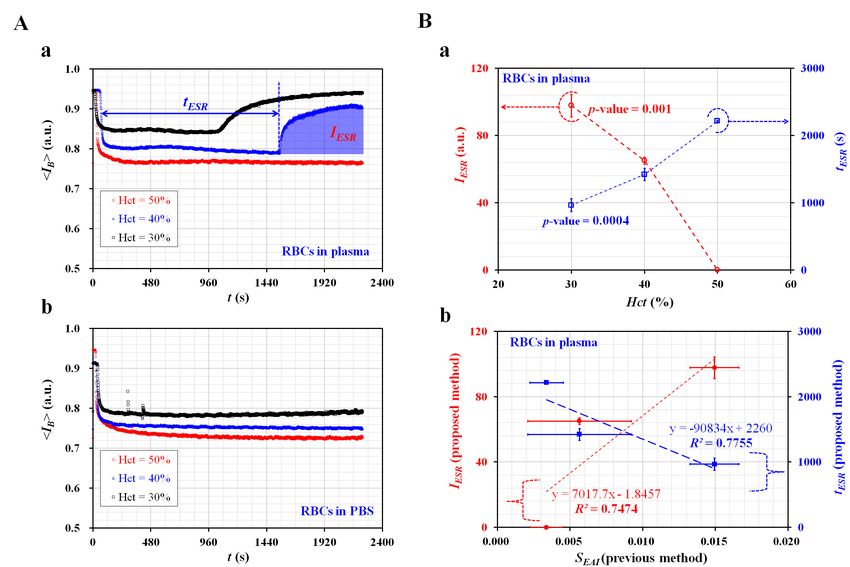
Micromachines 2020, 11, 215                                                                             2 of 25

       Under normal physiological conditions, red blood cells (RBCs) occupy 40–50% of blood volume.
As RBCs are the most abundant cells in the blood sample, the biophysical properties of the blood sample
are determined dominantly by properties of RBCs. The characteristics of RBCs, including morphology,
membrane viscoelasticity, and RBCs count, are evaluated by quantifying several biophysical properties
of blood samples, including viscoelasticity (or viscosity), deformability, and hematocrit. In that regard,
plasma proteins in blood samples induce RBC aggregation, which occurs at an extremely low shear
            .
rate (i.e., γ = 1~10 s−1 ) [10] or stasis. Among the biophysical properties of blood samples, blood
viscosity is determined by several factors, including hematocrit, plasma viscosity, RBCs deformability,
and RBCs aggregation. Thus, their properties of blood samples are employed to monitor variations in
the characteristics of blood samples. At lower shear rates, RBC aggregation causes to increase blood
viscosity. At high shear rates, the deformation and alignment of RBCs lead to a decrease in blood
viscosity. In other words, blood viscosity provides information on aggregation and deformability
simultaneously. However, at extremely low shear rates, a syringe pump (SP) exhibits fluidic instability
and RBC sedimentation continuously occurs. A microfluidics-based viscometer does not provide
consistent values of blood viscosity. Conventionally, blood viscosity has been measured at sufficiently
                        .                     .
high shear rates (i.e., γ > 10 s−1 [11,12] or γ > 50–100 s−1 [13,14]), especially in microfluidic environments.
For the reason, blood viscosity obtained with a microfluidic device does not give sufficient information
on the contributions of plasma proteins to RBC aggregation. To evaluate variations in plasma proteins
consistently, it is additionally necessary to quantify RBCs aggregation or ESR.
       A microfluidic device has several advantages, including small volume consumption,
fast measurement, easy sample handling, high sensitivity, and disposability. Thus, it has been widely used
to measure various biophysical properties of blood samples (i.e., blood viscosity [15], RBCs aggregation [16],
RBCs deformability [17,18], and hematocrit [19]).
       The previous methods for measuring blood viscosity are conveniently divided into three categories
(i.e., driving sources, devices, and quantification techniques). First, extrinsic driving sources such as
SPs [20], pressure sources, and hand-held pipettes [13] have been suggested for delivering a blood
sample into a specific device. Additionally, intrinsic driving sources such as capillary force (or surface
tension) [21,22] and gravity force [23] have been applied to supply blood samples into a device.
Second, various devices such as a microelectromechanical system (MEMS)-based microfluidic device,
a 3D-printed microfluidic device [13,24], and a paper-based device [25] have been suggested for
inducing blood flow in a specifically constrained direction. Third, quantification techniques such as
advancing meniscus (i.e., variations of a blood column over time) [15,22,26,27], the falling time of a
metal sphere in a tube [28], electric impedances (i.e., resistance, capacitance) [29,30], droplet length [31],
digital flow compartment with a microfluidic channel array [11,12], interface detection in co-flowing
streams [32,33], and reversal flow switching in a Wheatstone bridge analog of a fluidic circuit [14] have
been suggested to measure blood viscosity.
       To measure RBCs aggregation in microfluidic environments, a blood sample is placed into a
microfluidic channel. By applying shear stress to the blood sample with external driving systems
(i.e., an SP [34], pinch valve [16], or stirring motor [35]), the RBCs in the blood sample are aggregated
or disaggregated, depending on the shear rate. Several quantification methods, such as light
intensity (i.e., transmission, and back-scattering) [16], electrical conductivity [36,37], microscopic
RBC images [38–40], ultrasonic images [41], and optical tweezers [42] have been suggested for obtaining
temporal variations of RBCs aggregation. As another approach, RBC aggregation can be quantified by
measuring the sedimentation distances of RBCs in a blood sample during a specific duration (i.e., ESR).
Unlike the conventional Westergren ESR method, a microfluidic-based ESR measurement is quantified
by measuring the conductivity of the blood sample in a PDMS chamber with a square cross-section
(i.e., each side = 4 mm, depth = 5 mm) [43]. Owing to the continuous ESR in the driving syringe,
RBC-free regions (or depleted regions) expand from the top layer with an elapse of time. The blood
sample is supplied into a microfluidic device from the top layer of the driving syringe. To monitor
blood flows in the microfluidic channel, microscopic images are sequentially captured with a high speed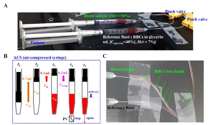
Micromachines 2020, 11, 215                                                                         3 of 25

camera. Image intensity of each microscopic image is calculated over time by conducting digital image
processing. The ESR is then evaluated by quantifying temporal variations of the image intensity [44].
     To measure blood viscosity and RBC aggregation inexpensively, two SPs should be replaced with
an inexpensive and disposable delivery system. To remove the syringe pump, single ACS is suggested
to infuse the blood sample into a microfluidic device for measuring pressure and RBCs aggregation
over continuously varying flow rates [45]. In this study, the ultimate goal of this study is to measure
blood viscosity and RBC aggregation (or ESR), without two SPs.
     In this study, a simple method for measuring blood viscosity and ESR is proposed. It involves the
quantification of the interfacial location in a co-flowing channel and microscopic image intensity of
blood sample flowing in a microfluidic device. Two air-compressed syringes (ACSs) are employed to
simultaneously deliver the blood sample and reference fluid. Based on an ACS for delivering blood
samples as suggested in previous studies [46,47], two ACSs are suggested to deliver blood samples and
reference fluid simultaneously. Since the flow rates of both fluids are not specified under fluid delivery
with the ACSs, it is necessary to quantify them with a time-resolved micro-particle image velocimetry
(µ-PIV) technique. Based on a parallel co-flowing method with a correction factor [32], the blood
viscosity is measured by monitoring the interfacial location in a co-flowing channel. Unlike the
previous studies [46,47], two ACSs are installed horizontally to measure ESR effectively. Continuous
sedimentation in the ACS causes an expansion of an RBC-free layer from the top layer. When blood
samples are delivered to the blood channel from the ACS, the populations of RBCs (or hematocrit) are
reduced over time. Since a continuous ESR contributes to increasing microscopic image intensity of
blood flows, the ESR can be quantified by monitoring the image intensity of the blood sample.
     When compared to previous methods that have the ability to measure blood viscosity under
fluid delivery with syringe pumps, two syringe pumps are replaced by two ACSs as a novelty of this
method. Here, a 40% glycerin solution is newly selected as the reference fluid. RBCs as fluid tracers
are added into reference fluid. Velocity fields of both fluids are obtained consistently over time by
conducting a time-resolved micro-PIV technique.
     By installing the ACSs horizontally, the continuous ESR inside the ACS is filled with the blood
sample causing it to expand RBC-free regions. As RBCs aggregation tends to increase substantially
at lower hematocrit or lower velocity, it contributes to increasing the image intensity of blood
samples. Thus, it is possible to evaluate the ESR by monitoring the microscopic image intensity of the
blood sample.

2. Materials and Methods

2.1. Fabrication of Microfluidic Device and Experimental Procedure
     A microfluidic device for measuring blood viscosity and ESR consisted of two inlets (a, b),
one outlet (a), and a T-shaped channel (width = 250 µm, depth = 20 µm), as shown in Figure 1A-a.
The T-shaped channel was composed of a blood channel, a reference channel, and a co-flowing channel.
When analyzing the velocity fields of each fluid, the T-shaped channel does not require to align
each microscopic image in the horizontal direction. Conventional micro-electromechanical-system
techniques, such as photolithography and deep reactive ion etching (DRIE), were employed to fabricate
4-inch silicon mold. To peel off PDMS block from the master mold easily, plasma surface treatment
was conducted after the DRIE process [48]. PDMS elastomer (Sylgard 184, Dow Corning, Midland,
MI, USA) was mixed with a curing agent at a ratio of 10:1. After positioning the mold on a petri dish,
the PDMS mixture was poured into the mold. Air bubbles dissolved in the PDMS were removed by
operating a vacuum pump (WOB-L Pump, Welch, Gardner Denver, Milwaukee, WI, and USA) for 1
h. After curing the PDMS in a convective oven at 70 ◦ C for 1 h, a PDMS block was peeled off from
the mold. It cut with a razor blade. Two inlets and outlets were punched with a biopsy punch (outer
diameter = 1.0 mm). After treating the surfaces of the PDMS block and a glass slide with an oxygen
plasma system (CUTE-MPR, Femto Science Co., Gyeonggi-do, Korea), the PDMS block was bonded on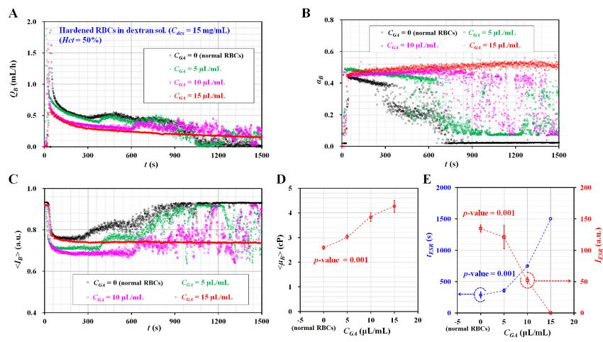
Micromachines 2020, 11, 215 4 of 25
Micromachines 2020, 11, x FOR PEER REVIEW 4 of 23
bonded on a glass substrate. A microfluidic device was finally prepared by placing it on a hotplate at
a glass substrate. A microfluidic device was finally prepared by placing it on a hotplate at 120 ◦ C for
120 °C for 10 min.
10 min.
Figure 1. Proposed
Proposed method
method forfor measuring
measuring blood blood viscosity
viscosity and and erythrocyte
erythrocyte sedimentation
sedimentation rate rate (ESR)
(ESR)
under fluid delivery of two air-compressed syringes (ACSs). (A) (A) Schematic
Schematic diagram
diagram of of the
the proposed
technique,
technique, including
including aa microfluidic device, two ACSs, and an an image
image acquisition
acquisition system.
system. (a) (a) AA
microfluidic
microfluidic devicedevice consisting
consisting of of two
two inlets
inlets (a,b),
(a,b), one
one outlet
outlet (a),
(a), and
and a T-shaped channel (i.e., blood
channel, reference
channel, referencechannel,
channel,and andco-flowing
co-flowing channel).
channel). (b)(b)Two TwoACSs ACSs for delivering
for delivering blood blood samples
samples and
and reference
reference fluid.fluid.
Each Each
ACS wasACScomposed
was composed of a disposable
of a disposable syringe syringe
(~1 mL),(~1amL), a fixture,
fixture, and a valve.
and a pinch pinch
valve.
(c) The(c) The microfluidic
microfluidic device device is located
is located in anin optical
an opticalimageimage acquisition
acquisition systemcomposed
system composedof of optical
optical
microscopy with a 20× objective lens (NA = 0.4), and a high-speed camera.
with a 20× objective lens (NA = 0.4), and a high-speed camera. The camera had a frameThe camera had a frame rate
of 5 kHz
rate and captured
of 5 kHz sequential
and captured snapshots
sequential at an interval
snapshots of 1 s. of
at an interval (B)1 Three
s. (B) regions-of-interest
Three regions-of-interest (ROIs)
were selected
(ROIs) for evaluating
were selected four parameters
for evaluating (,(,, URB,, Uand
R, andαB ).αB
). and
by conducting
by conducting digital image processing. U UBB and
and U URR were
were obtained
obtained by by conducting
conducting a micro-particle
image velocimetry (PIV) technique. (C) (C) As
As aa preliminary
preliminary demonstration,
demonstration, blood blood sample
sample (normal
(normal RBCsRBCs
in 10 mg/mL dextran solution (Hct = 50%)) and reference fluid (RBCs
in 10 mg/mL dextran solution (Hct = 50%)) and reference fluid (RBCs in 40% glycerin solution (Hct in 40% glycerin solution (Hct=
= 7%))
7%)) were were delivered
delivered to each
to each inletinlet
with with
twotwoACSs.ACSs. (a) Microscopic
(a) Microscopic images images captured
captured at a specific
at a specific time
time
(t) (t =(t)50, = 50,600,
(t 300, 300,900,
600,1200,
900, and
1200,1500 ands).1500 s). (b) Temporal
(b) Temporal variations variations
of of and.
and(c) . (c)
Temporal
Temporal variations of
variations of and αB. BSeparationand α . Separation time (T ) was obtained as the time
B time (Tst) was obtained as the time when started toB increase.
st when started
to increase. First, blood viscosity was evaluated from three
First, blood viscosity was evaluated from three parameters (UB, UR, and BαB) obtainedparameters (U , U R , and α ) obtained
Bwithin Tst.
within Tthe
Second, st . Second, the blood
ESR of the ESR ofsample
the blood wassample
evaluatedwasfrom
evaluated from obtained
Tst. above Tst .
As shown in Figure 1A-b, two polyethylene tubes (L ) (length = 300 mm, inner diameter = 500 µm,
As shown in Figure 1A-b, two polyethylene tubes 1(L1) (length = 300 mm, inner diameter = 500
and thickness = 500 µm) were tightly fitted into two inlets (a, b). The end of each tube was connected
μm, and thickness = 500 μm) were tightly fitted into two inlets (a, b). The end of each tube was
to the individual syringe needle of the ACS. The outlet of each ACS was clamped with a pinch valve.
connected to the individual syringe needle of the ACS. The outlet of each ACS was clamped with a
The other tube (L2 ) (length = 200 mm, inner diameter = 500 µm, and thickness = 500 µm) was tightly
pinch valve. The other tube (L2) (length = 200 mm, inner diameter = 500 μm, and thickness = 500 μm)
fitted into outlet (a). The end of the tube (L ) was connected to a waste dish. To remove air bubbles
was tightly fitted into outlet (a). The end of2the tube (L2) was connected to a waste dish. To remove
and avoid non-specific binding of plasma proteins to the inner surface of the channels, the channel was
air bubbles and avoid non-specific binding of plasma proteins to the inner surface of the channels,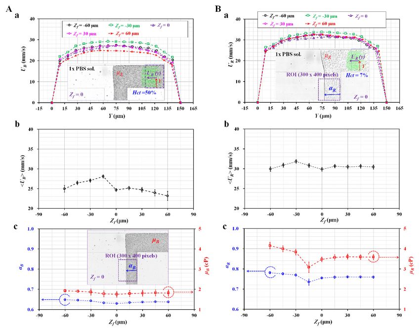
Micromachines 2020, 11, 215                                                                           5 of 25

filled with bovine serum albumin (BSA) solution (CBSA = 2 mg/mL) through outlet (a). After an elapse
of 10 min, the microfluidic channel was newly filled with 1× PBS.
      Based on the concept of ACS as reported in a previous study [45], two ACSs were employed to
deliver the blood sample and reference fluid into the microfluidic device. Figure A1A (Appendix A)
showed two ACSs filled with the blood sample (Hct = 50%) and reference fluid (RBCs suspended in
40% glycerin solution (Hct = 7%)). Each ACS was composed of a disposable syringe (~ 1 mL), a fixture,
and a pinch valve. Two pinch valves were used to stop or allow the fluid flow of each fluid. Each ACS
was placed horizontally on the stage of the optical microscope and fixed with an adhesive tape. Here,
an angle of inclination of the ACS only depended on an individual fixture. It was certain that the
installation angle of the ACS remained identical because the same fixture of the ACS was used for
all experiments.
      As shown in Figure A1B (Appendix A), the operation of each ACS was classified into five steps:
(1) piston movement at the lowest position forward at t = t1 , (2) air suction by moving the piston to
0.7 mL backward at t = t2 , (3) blood suction by moving the piston to 0.3 mL backward at t = t3 , (4) air
compression by moving the piston to 0.3 mL forward at t = t4 , and (5) blood delivery by removing the
pinch valve at t = t5 . As the air cavity inside the ACS was compressed to 0.3 mL, internal pressure
increased substantially above atmospheric pressure. Similarly, the reference fluid was sucked into
the syringe. The remainder of the procedure was the same as blood delivery. By removing two pinch
valves, blood sample and reference fluid were delivered to the corresponding inlets because pressure
difference increased inside the ACS.
      The microfluidic device was positioned on an optical microscope (BX51, Olympus, Tokyo, Japan)
equipped with a 20× objective lens (NA = 0.4). As shown in Figure 1A-c, a high-speed camera
(FASTCAM MINI, Photron, Tokyo, Japan) was used to obtain sequential microscopic images of the
blood sample and reference fluid flowing in the microfluidic channels. The camera offered a spatial
resolution of 1280 × 1000 pixels. Each pixel corresponded to 10 µm physically. A function generator
(WF1944B, NF Corporation, Yokohama, Japan) triggered the high-speed camera at an interval of 1 s.
Then, two microscopic images were captured at a frame rate of 5 kHz.
      To minimize the effect of temperature on blood viscosity, all experiments were conducted at a
room temperature of 25 ◦ C. Contributions of two factors (i.e., humidity, and atmospheric pressure) to
the present method were neglected. After the blood sample was injected into an ACS, the blood sample
did not contact with environment air. Additionally, the ACS was operated by pressure difference
(∆P) between pressure inside ACS (PACS ) and atmosphere pressure (Patm ) (i.e., ∆P = PACS − Patm ) [47].
The pressure difference depended on air volume inside the ACS (i.e., gauge pressure), rather than
atmospheric pressure.

2.2. Quantification of Microscopic Image Intensity, Blood Velocity Fields, and Interfacial Location
     First, blood viscosity was obtained by quantifying the velocity fields of blood sample flowing
in the blood channel, the velocity fields of reference fluid flowing in the reference channel, and the
interface location between two fluids flowing in the co-flowing channel.
     RBCs as fluid tracers were added into reference fluid to obtain the velocity fields of the reference
fluid. To measure velocity fields of reference fluid consistently, RBCs should be distributed uniformly
in reference fluid during experiments. According to previous studies [1,2], when reference fluid was
prepared by adding RBCs into 1× PBS and filled into the ACS, sedimentation of RBCs in ACS occurred
continuously over time. RBCs in reference fluid did not flow uniformly over time. After a certain lapse
of time, there were no fluid tracers in reference fluid. It was then impossible to obtain the velocity
fields of the reference fluid. To resolve the critical issue, a 40% glycerin solution was carefully selected
as a base solution in reference fluid. Additionally, to minimize contributions of RBCs to velocity fields
and viscosity, hematocrit of RBCs added into reference fluid was fixed at Hct = 7%.
     As shown in Figure 1B, an ROI (300 × 300 pixels) was selected to obtain the velocity fields of the
blood sample flowing in the blood channel. Another ROI with 300 x 300 pixels was selected to obtain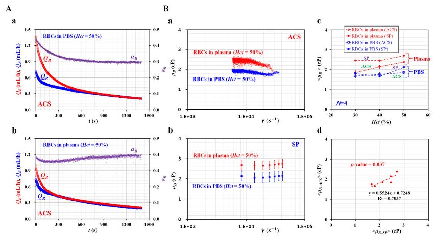
Micromachines 2020, 11, 215                                                                           6 of 25

the velocity fields of the reference fluid flowing in the reference channel. By conducting a time-resolved
µPIV technique, the velocity fields of the blood sample (UB ) across the blood channel width were
obtained over time. Additionally, velocity fields of the reference fluid flow (UR ) across the reference
channel width were obtained over time. The size of the interrogation window was selected as 64 × 64
pixels. The window overlap was set to 75%. The velocity fields were validated and corrected with a
median filter. The averaged velocities (, ) of both fluids were calculated as an arithmetic
average over the specific ROI. To obtain the interface (i.e., blood sample-filled width) in the co-flowing
channel (αB ), an ROI with 300 × 400 pixels was selected in the co-flowing channel. A gray-scale
microscopic image was converted into a binary image by adopting Otsu’s method [49]. By conducting
an arithmetic average over the ROI, variations of the interfacial location in the co-flowing channel (αB )
were obtained over a period of time.
     Second, the ESR was evaluated by quantifying the microscopic image intensity of the blood
sample flowing in the blood channel. To evaluate the microscopic image intensity of blood flows, and
ROI with 300 x 300 pixels was selected in the blood channel. The image intensity of the blood sample
flowing in the blood channel was obtained by conducting digital image processing with a commercial
software package (Matlab 2019, Mathworks, Natick, MA, USA). An averaged value of microscopic
image intensity () was obtained by performing an arithmetic average of image intensity over the
specific ROI.

2.3. Quantification of Blood Viscosity and ESR
     As a preliminary demonstration, blood samples (normal RBCs suspended in specific dextran
solution (10 mg/mL), Hct = 50%) and reference fluid were delivered to the corresponding inlets (a, b)
under the fluid delivery with two ACSs. To visualize the velocity fields of the reference fluid flowing
in the reference channel, the reference fluid was prepared by adding normal RBCs (Hct = 7%) into a
40% glycerin solution.
     Figure 1C-a showed microscopic images captured at specific times (t) (t = 50, 300, 600, 900,
1200, and 1500 s). Above t = 600 s, the populations of RBCs flowing in the blood channel decreased
substantially over time. As shown in Figure 1C-b, temporal variations of UB and UR were obtained by
conducting the µPIV technique. As the pressure difference between the inner pressure and atmospheric
pressure tended to decrease over time in the ACS, the averaged velocity of the reference fluid ()
tended to decrease stably over time. However, owing to the continuous ESR inside the ACS, an RBC-free
liquid was observed in a tube, as shown in Figure A1C (Appendix A). The averaged velocity of the
blood sample () varied unstably above t = 400 s. Figure 1C-c showed the temporal variations in
the image intensity of the blood sample flowing in the blood channel (), and the interface between
the two fluids in the co-flowing channel (αB ). Similar to UB , the continuous ESR inside the ACS led to
unstable behaviors in  and αB . In this study, the separation time when unstable behavior began
was denoted as Tst . At t < Tst , three factors (, , and ) exhibited stable variations over
time. Thus, the blood viscosity was quantified from the three factors (, , and αB ). For a
rectangular channel with an extremely low aspect ratio, an approximate formula of fluidic resistance
                                       12 µ L
was derived approximately as R = w hB3 . A co-flowing channel was filled with a blood sample and
reference fluid, respectively. For simple mathematical representation, both streams were represented
as two fluidic resistances connected in parallel. The corresponding fluidic resistance for each fluid was
                  12 µ L                                   12 µ L
derived as RB = Wα Bh3 for a blood sample, and RR = W (1−αR ) h3 for reference fluid. Here, µR meant the
                      B                                        B
viscosity of the reference fluid. As both fluids had the same       Q  drop (i.e., ∆P = RB ·QB = RR ·QR ),
                                                            α pressure
blood viscosity formula (µB ) was derived as µB = µR × 1−αB B × QRB . Here, QB and QR represented the
flow rate of the blood sample and reference fluid, respectively. The simple mathematical model did not
account for real boundary conditions in co-flowing flows. Thus, to compensate for the deviation from
the real boundary condition, the previous study included a correction factor in the analytical formula of
blood viscosity. According to the blood viscosity formula reported in a parallel co-flowingmethod with
                                                                                               α       Q

a correction factor [32], the blood viscosity formula (µB ) was modified as µB = C f × µR × 1−αB B × QRB .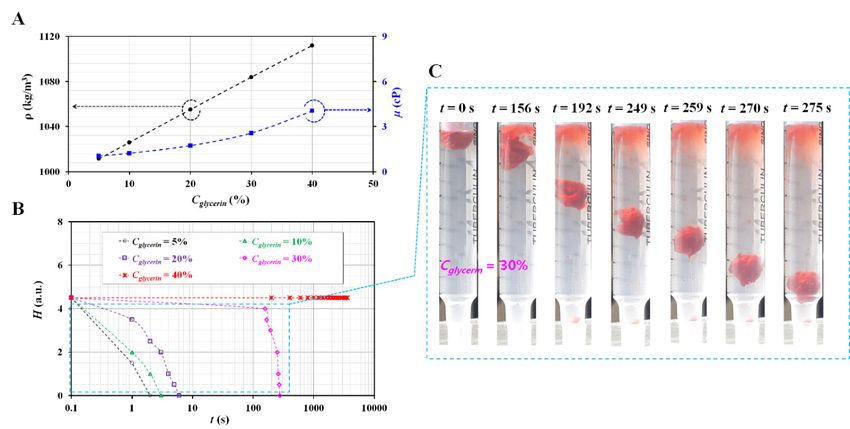
Micromachines 2020, 11, 215                                                                            7 of 25

Since the correction factor (Cf ) was varied depending on the channel size, a numerical simulation was
conducted to determine the correction factor. Based on a procedure discussed in a previous study [32],
a numerical simulation using commercial computational fluid dynamics (CFD) software (CFD ACE+,
ESI Group, Paris, France) for a rectangular channel (width = 250 µm, depth = 20 µm) was conducted to
obtain the viscosity of the test fluid with respect to the interface. For convenience, it was assumed
that the reference fluid and test fluid behaved as Newtonian fluids. Both fluids had the same value,
as µref = µtest = 1 cP. The interface between both fluids was relocated by varying the flow rate ratio of
the reference fluid to test fluid. As shown in Figure A2A (Appendix A), when the interface moved
from center line (αx = 0.5) to each wall (i.e., αx = 0 or 1), the blood viscosity without the correction
factor (i.e., µn ) showed a large deviation when compared with the viscosity of the test fluid (µtest = 1
cP). Considering that the viscosity of the test fluid should have a constant value of µtest = 1 cP with
respect to the interface, the correction factor (Cf ) could be obtained by reciprocating µn with respect to
αx (i.e., Cf = 1/µn ). By conducting a regression analysis, the variations of the correction factor with
respect to the interface were obtained as C f = 9.7212αx 4 − 19.442αx 3 + 15.687αx 2 − 5.9659αx + 1.8992
(R2 = 0.9968). As shown in Figure A2B (Appendix A), to validate Cf , the viscosities of the test fluid
were given as (a) µtest = 1 cP and (b) µtest = 4.08 cP. The flow rates of both fluids were the same, at 1
mL/h (i.e., Qref = Qtest = 1 mL/h). By applying the correction factor, the viscosities of the test fluids were
determined as 1 cP and 4.14 cP, respectively. From the results, it was found that the parallel co-flowing
method with the correction factor had the ability to measure the viscosity of a test fluid within 1.4%
of a normalized difference. However, at t > Tst , the continuous ESR inside the ACS caused unstable
behaviors in blood flows. To quantify the ESR, two indices (i.e., IESR, TESR ) were suggested from
and Tst , as shown in Figure 5. Based on previous studies [45,50], one ESR index (IESR ) was suggested
                                                                   R t=T
simply by integrating  from t = Tst to t = Tend (i.e., IESR = t=T end < IB >dt). Here, Tend represented
                                                                       st
the end time of each experiment. Additionally, TESR = Tst − Ti . Ti indicated the initial time when the
blood sample started to fill the blood channel.
      From the preliminary demonstration, four factors (, , αB , and ) could be effectively
employed to obtain the blood viscosity and ESR when two ACSs were employed to deliver the blood
sample and reference fluid into a microfluidic device.

2.4. Selection of Base Solution in Reference Fluid
      To visualize the velocity fields of the reference fluid, RBCs were added into the reference fluid as
fluid tracers. Glycerin solution was suggested as a reference fluid to minimize the sedimentation of
RBCs inside the ACS. According to a previous study [51], the density (ρ) and viscosity (µ) increased
at higher concentrations of glycerin solution as shown in Figure A3A (Appendix A). To evaluate the
sedimentation rate of the RBCs added into the reference fluid, a simple ESR tester was prepared by using
a disposable syringe (~1 mL) as shown in Figure A3C (Appendix A). The disposable syringe was fitted
vertically into a hole (outer diameter = 4 mm) of the PDMS block. The outlet of the hole was closed with
3M adhesive tape. The syringe was filled with a specific concentration of glycerin solution (~0.5 mL).
A 50 µL RBCs droplet was dropped into a specific concentration of glycerin solution. To monitor the
sedimentation rate of the RBCs droplet in the simple ESR tester, snapshots were captured at an interval
of 1 s with a smartphone camera (Galaxy A5, Samsung, Korea). As shown in Figure A3B (Appendix A),
temporal variations of sedimentation height (H) were obtained by varying the concentration of the
glycerin solution (Cglycerin ) (Cglycerin = 5%, 10%, 20%, 30%, and 40%). Figure A3C (Appendix A) showed
sedimentation of the RBCs droplet in 30% glycerin solution over time (t) (t = 0, 156, 192, 249, 259, 270,
and 275 s). From the results, the RBCs droplet in the 40% glycerin solution remained nearly identical at
the upper position, even without sedimentation. Furthermore, considering that the densities of normal
RBCs range from 1090 kg/m3 to 1106 kg/m3 [52], the reference fluid was selected as a 40% glycerin
solution (Cglycerin = 40%), because its density was greater than that of the RBCs.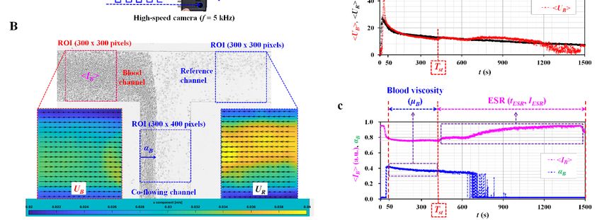
Micromachines 2020, 11, 215                                                                            8 of 25

2.5. Statistical Analysis
      The statistical significance was evaluated by conducting statistical analyses with a commercial
software package (Statistical Package for the Social Sciences (SPSS) Statistics version 24, IBM Corp.,
Armonk, NY, USA). Two ESR indices (IESR , TESR ) and blood viscosity () obtained by the present
method were compared with results reported in a previous study (i.e., blood viscosity: µB , ESR
index: SEAI ). An analysis of variance (ANOVA) test was applied to verify significant differences
between comparative results. A linear regression analysis was conducted to verify the correlations
between two parameters. All experimental results were expressed as mean ± standard deviation.
If the p-value was less than 0.05, the experimental results exhibited significant differences within a 95%
confidence interval.

3. Results and Discussion

3.1. Contribution of RBCs Added into Reference Fluid to Viscosity and Velocity Fields
       To evaluate the effects of the RBCs added into the reference fluid on fluid viscosity, the viscosity
of the reference fluid was measured by varying the volume of the RBCs added to the reference fluid
(i.e., hematocrit [Hct]). In that regard, a 1× PBS was delivered to the blood channel (i.e., left-side
channel) at a constant flow rate of QPBS = 1 mL/h with a syringe pump (SP) (neMESYS, Centoni Gmbh,
Germany). The hematocrit (Hct) of the reference fluid was adjusted to Hct = 3%, 5%, 7%, and 9% by
adding normal RBCs into the 40% glycerin solution. The reference fluid was delivered to the reference
channel (i.e., right-side channel) at a constant flow rate of Qglycerin = 1 mL/h with an SP. Figure 2A
showed microscopic images for evaluating the interfacial location in the co-flowing channel with
respect to Hct ((a) Hct = 0%, (b) Hct = 3%, (c) Hct = 5%, (d) Hct = 7%, and (e) Hct = 9%). To verify the
contribution of the hematocrit in the reference fluid to the velocity fields (UR ), the velocity fields of the
reference fluid were obtained across the reference channel width with respect to Hct. As shown in
Figure 2B-a, a variation of the velocity profile (UR ) was obtained across the reference channel width with
respect to Hct. The inset showed the microscopic image and velocity profile of the reference fluid with
Hct = 3%. From the results, the velocity profile did not show a distinctive difference depending on the
hematocrit. Figure 2B-b showed variations of the averaged velocity of the reference fluid () with
respect to Hct. The hematocrit in the reference fluid did not contribute to varying  significantly.
As shown in Figure 2C-a, the variations of the interface in the co-flowing channel (αR ) and the viscosity
(µR ) were obtained with respect to Hct. The interface and viscosity remained constant as αR = 0.771 ±
0.003 and µR = 3.868 ± 0.068 cP for the reference fluid, with up to 9% hematocrit. From the results, it
could be observed that providing up to a 9% hematocrit in the reference fluid did not significantly
contribute to increasing the viscosity of the reference fluid. In addition, as shown in Figure A3A
(Appendix A), an empirical formula [51] indicated that a 40% glycerin solution without any RBCs had
a viscosity value of 4.07 cP. Based on the parallel co-flowing method with the correction factor [32], the
viscosity of the reference fluid was measured consistently within a 5% difference when compared with
the empirical formula. Furthermore, a previous flow-switching method [14] was employed to measure
the viscosity of the reference fluid with respect to hematocrit. The inset of Figure 2C-b showed reversal
flow-switching in the junction channel for the reference fluid with Hct = 7%. By increasing the flow
rate of the 1× PBS (QPBS ) from QPBS = 1 mL/h to QPBS = 3.1 mL/h, the hydrodynamic balancing in
both side channels caused to reverse flow direction from left direction to right direction (i.e., reversal
flow-switching phenomena) [14]. In other words, the junction channel was filled with blood at QPBS
= 1 mL/h. However, it was filled with 1× PBS at QPBS = 3.1 mL/h. Based on the viscosity formula
suggested in the flow-switching method, the viscosity of the reference fluid was quantified as µR =
3.1 ± 0.05 cP. As shown in Figure 2C-b, the viscosity obtained by both methods remained stable, with
respect to hematocrit. Similar to the case in the parallel co-flowing method with the correction factor,
the results of the flow-switching method indicated that the RBCs added into the reference fluid did not
contribute to varying the viscosity within 9% hematocrit. The viscosity obtained by the flow-switching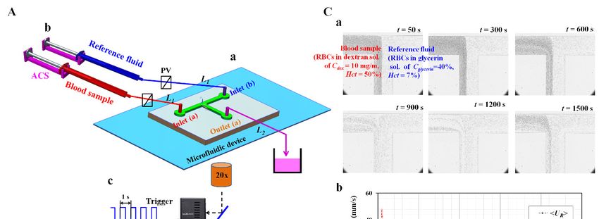
Micromachines 2020, 11, 215 9 of 25
Micromachines 2020, 11, x FOR PEER REVIEW 9 of 23
method was underestimated by approximately 20% when compared with that obtained by the parallel
in this study,method
co-flowing the reference
with thefluid was prepared
correction by adding
factor. From thesenormal
results,RBCs
in this(Hct = 7%)
study, theinto a 40% fluid
reference glycerin
was
prepared by adding normal RBCs (Hct = 7%) into a 40% glycerin solution throughout all experiments.
solution throughout all experiments.
ContributionsofofRBCs
Figure2.2.Contributions
Figure RBCsaddedaddedinto intothe
thereference
referencefluidfluidtotoviscosity.
viscosity. 1× 1×PBS
PBSwas wasdelivered
deliveredto to
theblood
the bloodchannel
channelatataaconstant
constantflow flowrate
rateofof11mL/h
mL/hwith withaasyringe
syringepumppump(SP). (SP).The
Thehematocrit
hematocrit(Hct)(Hct)ofof
referencefluid
reference fluidwas
wasadjusted
adjustedby byadding
addingnormal
normalRBCs RBCsinto into40%40%glycerin
glycerinsolution (Hct==0,0,3%,
solution(Hct 3%,5%,
5%,7%,
7%,
and9%).
and 9%).TheThereference
referencefluid
fluidwas
wasdelivered
deliveredtotothe thereference
referencechannel
channelatataaconstant
constantflowflowraterateof
of11mL/h
mL/h
with an SP. (A) Microscopic images for obtaining interface (α ) in co-flowing
with an SP. (A) Microscopic images for obtaining interface (αR) Rin co-flowing channel with respect to channel with respect
to Hct
Hct = 0,= (b)
HctHct
((a)((a) HctHct
0, (b) = 3%,
= 3%, (c)(c)
HctHct== 5%,5%,(d)(d)HctHct= =7%,
7%,andand(e) Hct==9%).
(e)Hct 9%).(B)(B)Contributions
Contributionsof of
hematocritin
hematocrit inreference
referencefluid
fluid to
tovelocity
velocity fields
fields (U(URR).).(a)
(a)Variation
Variationof ofvelocity
velocityfields
fields(U(URR) )across
acrossreference
reference
channelwidth
channel widthwithwithrespect
respecttoto Hct.
Hct. TheThe inset
inset showed
showed a microscopic
a microscopic image image
andand a velocity
a velocity profile
profile of
of the
the reference fluid with Hct = 3%. (b) Variations
reference fluid with Hct = 3%. (b) Variations of averaged of averaged over a region of interest
over a region of interest (ROI) with (ROI)
with respect
respect Hct.
to Hct.to(C) Effect of HctofinHct
(C) Effect in reference
reference to fluid
to fluid on viscosity
on viscosity (µRVariations
(μR). (a) ). (a) Variations
of αR of αRμand
and µR
R with
with respect
respect to Hct. Hct.Comparison
to (b) (b) Comparison between
between the the proposed
proposed method
method (i.e.,
(i.e., thethe parallel-flowmethod
parallel-flow methodwithwith
correctionfactor)
correction factor)andandprevious
previousmethod
method(i.e.,(i.e.,flow-switching
flow-switching method)method) with with respect
respect to Hct.
to Hct.
3.2. Relationship between Flow Rate of Syringe Pump and Averaged Velocity Obtained by µPIV
3.2. Relationship between Flow Rate of Syringe Pump and Averaged Velocity Obtained by μPIV
To obtain blood viscosity, the flow rates of the blood sample and reference fluid should be
To obtain blood viscosity, the flow rates of the blood sample and reference fluid should be
measured from the averaged velocity obtained by conducting the µPIV technique. In other words,
measured from the averaged velocity obtained by conducting the μPIV technique. In other words,
there was a need to obtain the relationship between the flow rate delivered by the SP (Q ) and the
there was a need to obtain the relationship between the flow rate delivered by the SP (Qspsp) and the
averaged velocity obtained by conducting the µPIV technique ().
averaged velocity obtained by conducting the μPIV technique ().
The hematocrit of the blood sample was adjusted to Hct = 30%, 40%, and 50% by adding normal
RBCs into the base solution (1× PBS, plasma). Using two SPs, the flow rate of each fluid decreased
stepwise from Qsp = 1.5 mL/h to Qsp = 0.1 mL/h, at an interval of 0.2 mL/h. With respect to each flow
rate, the SP had been operated for 8 min. The blood sample was prepared by adding normal RBCs
into plasma. As shown in Figure 3A-a, temporal variations of the averaged velocity () and the
flow rate of the SP (Qsp) were obtained by varying the hematocrit. At a higher flow rate of Qsp, the
hematocrit contributed to decreasing . At a lower flow rate of Qsp, remained constant,
without contribution from the hematocrit. By changing the base solution from plasma to a 1× PBS,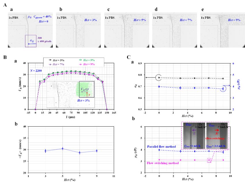
Micromachines 2020, 11, 215                                                                         10 of 25

      The hematocrit of the blood sample was adjusted to Hct = 30%, 40%, and 50% by adding normal
RBCs into the base solution (1× PBS, plasma). Using two SPs, the flow rate of each fluid decreased
stepwise from Qsp = 1.5 mL/h to Qsp = 0.1 mL/h, at an interval of 0.2 mL/h. With respect to each
flow rate, the SP had been operated for 8 min. The blood sample was prepared by adding normal
RBCs into plasma. As shown in Figure 3A-a, temporal variations of the averaged velocity () and
the flow rate of the SP (Qsp ) were obtained by varying the hematocrit. At a higher flow rate of Qsp ,
the hematocrit contributed to decreasing . At a lower flow rate of Qsp ,  remained constant,
without contribution from the hematocrit. By changing the base solution from plasma to a 1× PBS,
temporal variations of  and Qsp were obtained with respect to Hct. As shown in Figure 3A-b,
the variations of , with respect to hematocrit, were very similar to those of a blood sample
composed of plasma. By averaging  with respect to Qsp ,  was quantified as mean ± standard
deviation with respect to Qsp . To determine the relationship between  and Qsp , a scatter plot was
used to plot  on a vertical axis and Qsp on a horizontal axis. Figure 3A-c showed variations of
 with respect to Qsp and Hct in a blood sample composed of plasma. For example,  was
estimated as about 30 mm/s for Qsp =1.3 mL/h. Based on formula of flow rate (i.e., QµP = Ac ,
Ac = w x h), flow rate obtained by µPIV was estimated as QµPIV = 0.54 mL/h. When compared with
Qsp =1.3 mL/h, the normalized difference between Qsp and QµPIV was estimated as 59%. In this study,
instead of the flow rate formula, the flow rate of the blood sample or reference fluid was estimated
from the calibration formula obtained in advance. Thus, it was necessary to determine the relationship
between velocity () and Qsp . A regression analysis was conducted by assuming the regression
formula as a quadratic model. Regression formulas between  and Qsp with respect to Hct were
obtained, as shown inside of Figure 3A-c. The regression formulas for each hematocrit were obtained
as  = −5.027 Qsp 2 + 30.279 Qsp (R2 = 0.998) for Hct = 30%,  = −6.262 Qsp 2 + 30.660 Qsp (R2 =
0.999) for Hct = 40%, and  = −5.916 Qsp 2 + 29.137 Qsp (R2 = 0.999) for Hct = 50%. Figure 3A-d
showed variations of  with respect to the Qsp and Hct in a blood sample composed of 1× PBS.
From the regression analysis, as shown inside Figure 3A-d, the regression formulas for each hematocrit
were obtained as  = −4.850 Qsp 2 + 30.791 Qsp (R2 = 0.998) for Hct = 30%,  = −7.897 Qsp 2
+ 33.519 Qsp (R2 = 1.000) for Hct = 40%, and  = −5.717 Qsp 2 + 29.286 Qsp (R2 = 0.999) for Hct
= 50%. For the same hematocrit, the base solution (i.e., plasma or 1× PBS) did not contribute to
varying the coefficients of the quadratic formula (i.e., normalized difference < 4% except Hct = 40%).
However, for the same base solution, the coefficients of a quadratic model varied significantly with
respect to hematocrit.
      A regression formula between Qsp and  for the reference fluid (i.e., 40% glycerin solution)
with RBCs (Hct = 7%) was obtained by using a similar procedure to that used for the blood sample.
Figure 3B-a showed the temporal variations of Qsp and  for the reference fluid.  was
obtained as a mean ± standard deviation for a corresponding Qsp . When compared with the blood
sample,  increased substantially, owing to the lower value of the hematocrit. As shown in
Figure 3B-b, variations of  with respect to Qsp were represented by a scatter plot. From a
regression analysis, the regression formula between  and Qsp was obtained as  = −7.770
Qsp 2 + 37.127 Qsp (R2 = 0.9875).
      From the results, the coefficients of the quadratic formula were varied significantly with respect to
hematocrit. However, the base solution (i.e., 1× PBS, or plasma) did not contribute to changing the
coefficients of the regression formula. Using regression formulae between Qsp and  (or )
obtained in advance, the  or  obtained by conducting the µPIV technique was converted
into a flow rate (i.e., QB , QR , respectively).
analysis, as shown inside Figure 3A-d, the regression formulas for each hematocrit were obtained as
= −4.850 Qsp2 + 30.791 Qsp (R2 = 0.998) for Hct = 30%, = −7.897 Qsp2 + 33.519 Qsp (R2 = 1.000) for
Hct = 40%, and = −5.717 Qsp2 + 29.286 Qsp (R2 = 0.999) for Hct = 50%. For the same hematocrit, the
base solution (i.e., plasma or 1× PBS) did not contribute to varying the coefficients of the quadratic
formula (i.e.,2020,
Micromachines normalized
11, 215 difference < 4% except Hct = 40%). However, for the same base solution, the
11 of 25
coefficients of a quadratic model varied significantly with respect to hematocrit.
Figure 3. Calibration
Calibrationformula
formula
forfor
thethe relationship
relationship between
between flowcontrolled
flow rate rate controlled
by SP (Qby SP (Qsp) and
Figure 3. sp ) and averaged
averaged velocity obtained by μPIV technique (). Hematocrit (Hct) of blood was adjusted
velocity obtained by µPIV technique (). Hematocrit (Hct) of blood was adjusted to Hct = 30%, to40%,
Hct
=and
30%, 40%, and 50% by adding normal RBCs into a base solution (1× PBS or plasma).
50% by adding normal RBCs into a base solution (1× PBS or plasma). With two syringe pumps, With two
the flow rate of each fluid decreased stepwise from Qsp = 1.5 mL/h to Qsp = 0.1 mL/h at an interval
of 0.2 mL/h. Each flow rate was maintained for 8 min. (A) Relationship between Qsp and with
respect to hematocrit and base solution. (a) Temporal variations in and Qsp of blood sample
(normal RBCs in plasma) with respect to Hct. (b) Temporal variations in and Qsp of blood sample
(normal RBCs in 1× PBS) with respect to Hct. (c) Regression formula between and Qsp of blood
sample (normal RBCs in plasma) with respect to Hct. (d) Regression formula between and Qsp of
blood sample (normal RBCs in 1× PBS) with respect to Hct. (B) Calibration formula of relationship
between Qsp and of reference fluid (40% glycerin solution with RBCs (Hct = 7%). (a) Temporal
variations of Qsp and . (b) Regression formula between and Qsp .
3.3. Quantitative Comparison of Blood Viscosity with Respect to Fluid Delivery System (ACS, SP)
Since the and obtained from the µPIV technique were converted into flow rates (QR and
QB ) from regression formulae obtained in advance, the blood viscosity could be measured by monitoring
the interface (αB ) in the co-flowing channel, under fluid delivery with an ACS. The blood viscosity
obtained by the ACS was quantitatively compared with one obtained by an SP. Blood samples (Hct = 30%,
40%, and 50%) were prepared by adding normal RBCs into the base solution (1× PBS, plasma).
Figure 4A-a showed the temporal variations of QR , QB , and αB for the blood sample (normal RBCs
in 1× PBS, Hct = 50%). In addition, Figure 4A-b depicted the temporal variations of QR , QB , and
αB for the blood sample (normal RBCs in plasma, Hct = 50%). Using the blood viscosity formula,
the blood viscosity was obtained by using the temporal variations of QR , QB , and αB. Here, the viscosity
of the reference fluid was given as µR = 4.08 cP by using measurement results reported in previousMicromachines 2020, 11, 215 12 of 25
studies [14,51]. For a rectangular channel (width = w, depth = h) with a lower aspect ratio [32],
. . 6Q
the formula of shear rate (γ) was given as approximately γ = whB2 . The corresponding shear rate
of the blood viscosity obtained at a specific blood flow rate (QB ) was estimated by using the shear
.
rate formula. A scatter plot was employed to plot µB on a vertical axis, and γ on a horizontal axis.
As shown in Figure 4B-a, variations of µB were obtained with respect to the shear rate under fluid
delivery with the two ACSs. Here, the blood sample (Hct = 50%) was prepared by adding normal
RBCs into plasma or 1× PBS. The blood sample has behaved as a Newtonian fluid at sufficiently higher
.
shear rates (γ > 103 s−1 ). From the experimental results, µB remained constant with respect to the
shear rate. By conducting an arithmetic average of µB over specific shear rates, the blood viscosity
was expressed as = mean ± standard deviation. The viscosity of the blood sample composed
of plasma ( = 2.381 ± 0.042 cP) was significantly higher than that of the blood sample
composed of 1× PBS ( = 1.845 ± 0.0573 cP). To compare with the blood viscosity obtained
under fluid delivery with two ACSs, the same blood samples were employed to measure the blood
viscosity under fluid delivery with two SPs. Two fluids (blood sample, reference fluid) were delivered
to each inlet2020,
Micromachines of the
11, xmicrofluidic device, at the same flow rate (QB = QR ).
FOR PEER REVIEW 12 of 23
Figure 4. Quantitative
Quantitative comparison
comparison of of blood
blood viscosity
viscosity for
for blood
blood samples
samples (normal
(normal RBCs
RBCs in plasma and
PBS, Hct = = 50%) with
withrespect
respecttotothe
thefluid
fluiddelivery
delivery system (ACS, SP). (A) Variations
system (ACS, SP). (A) Variations of flow of flow
ratesrates
(QB ,(Q
QRB,)
Q R) and
and interface
interface (αB) with
(αB ) with respect
respect to thetobasethesolution
base solution (1×plasma).
(1× PBS, PBS, plasma). (a) Temporal
(a) Temporal variationsvariations
of QB , Qof
R,
Q
and αRB, for
B, Q anda αblood
B for a blood (normal
sample sample (normal
RBCs in 1× RBCsPBS,inand Hct =and
1× PBS, 50%).Hct(b)
= 50%). (b) Temporal
Temporal variations variations
of QB , QR ,
of
and QBα, BQfor
R, and αB forsample
a blood a blood sampleRBCs
(normal (normal RBCs inand
in plasma, Hct =and
plasma, Hct(B)
50%). = 50%). (B) Variation
Variation of blood
of blood viscosity
viscosity
depending depending
on the base onsolution,
the basehematocrit,
solution, hematocrit, and fluid
and fluid delivery delivery
system (ACSsystem
and SP).(ACS and SP). (a)
(a) Variations of
Variations
blood viscosity of blood
(µB ) viscosity (μB) of blood
of blood samples with samples
respect towith respect
the base to the(1×
solution base solution
PBS, plasma)(1×and
PBS,shear
plasma)
rate
under
and shearfluidrate
delivery
underoffluid
ACS.delivery
(b) Variations
of ACS. µB Variations
of (b) with respectoftoμBthe base
with solution
respect to (1× PBS, plasma)
the base solution and
(1×
shearplasma)
PBS, rate underandfluid
sheardelivery of two
rate under SPs.
fluid (c) Variations
delivery of Variations
(c) with respect toBbase
of withsolution
respect(1×
to
PBS, solution
base plasma),(1× hematocrit (Hct =hematocrit
PBS, plasma), 30%, 40%,(Hct and=50%), and fluid
30%, 40%, delivery
and 50%), andsystem (ACS, SP).
fluid delivery was
quantified
SP). was as = mean
quantified ± standard
as = meandeviation
± standard bydeviation
conducting by an arithmeticanaverage
conducting arithmeticof µaverage
B obtainedof
over
μ shear rates.
B obtained (d) Correlation
over shear rates. (d) between
Correlation blood viscosity
between obtained
blood viscosityunder ACS () and
()
viscosity
and bloodobtained
viscosityunder SP ().().
As represented
As represented in
in Figure
Figure 3A-a
3A-a and
and Figure
Figure 3A-b,
3A-b, the
the flow
flow rate
rate of
of the
the SP
SP (Q
(Qsp ) decreased stepwise
sp) decreased stepwise
from Q = 1.5 mL/h to Q = 0.1 mL/h at an interval of 0.2 mL/h. Each flow rate had
from Qsp = 1.5 mL/h to Qsp = 0.1 mL/h at an interval of 0.2 mL/h. Each flow rate had been
sp sp been maintained
maintained
for 8 min. As shown in Figure 4B-b, variations in µ of the blood samples (normal
for 8 min. As shown in Figure 4B-b, variations in μBB of the blood samples (normal RBCs in RBCs in plasma
plasma
and 1× PBS, Hct = 50%) were obtained with respect to the shear rate. The blood viscosity remained
constant with respect to the shear rate. The viscosity of the blood sample composed of plasma ( = 2.728 ± 0.0918 cP) was higher than that of the blood sample composed of 1× PBS ( =
2.109 ± 0.0429 cP). When compared with the blood viscosity obtained by the ACS, blood viscosity
obtained by the SP increased by approximately 12.5%. To determine the effects of hematocrit on bloodMicromachines 2020, 11, 215 13 of 25
and 1× PBS, Hct = 50%) were obtained with respect to the shear rate. The blood viscosity remained
constant with respect to the shear rate. The viscosity of the blood sample composed of plasma
( = 2.728 ± 0.0918 cP) was higher than that of the blood sample composed of 1× PBS
( = 2.109 ± 0.0429 cP). When compared with the blood viscosity obtained by the ACS,
blood viscosity obtained by the SP increased by approximately 12.5%. To determine the effects of
hematocrit on blood viscosity, variations of blood viscosity were obtained by varying the hematocrit
(Hct = 30%, 40%, and 50%), base solution (1× PBS, plasma), and fluid delivery system (ACS, SP).
Figure 4B-c showed the variations of with respect to Hct, base solution, and the fluid delivery
system. Under fluid delivery with an ACS, tended to increase with respect to Hct. Under fluid
delivery with an SP, there was no significant difference between Hct = 30% and Hct = 40%. The blood
viscosity increased at Hct = 50% when compared with Hct = 30% or 40%. To determine the correlation
between the blood viscosity obtained by the ACS () and the blood viscosity obtained by the
SP (), a scatterplot was used to plot on a vertical axis, and on a horizontal
axis, as shown in Figure 4B-d. According to a linear regression analysis, was expressed as
= 0.5524 + 0.7248 (R2 = 0.7037, p-value = 0.037). Here, p-value = 0.037 indicated
that a linear regression showed sufficient relationship between two viscosity values (i.e.,
vs. ). In addition, R2 was obtained as a high value of R2 = 0.7037. Although two SPs were
effectively used to deliver two fluids during measurement of blood viscosity, the arrangement included
challenges, such as a bulky size and a high cost. From the correlation between and ,
it was found that the ACS can be effectively employed to deliver two fluids in the measurement of
blood viscosity. Thus, the blood viscosity can be measured consistently under fluid delivery with
two ACSs.
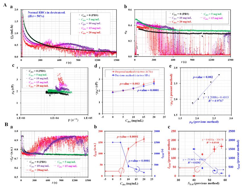
3.4. Quantitative Measurement of ESR with Respect to base Solution and Hematocrit
The ESR of the blood sample was evaluated by quantifying the microscopic image intensity of
the blood sample () flowing in the blood channel. Two ESR indices (tESR , IESR ) were suggested
by quantifying the temporal variations of . The blood samples (Hct = 30%, 40%, and 50%) were
prepared by adding normal RBCs into a base solution (1× PBS, plasma).
As shown in Figure 5A-a, variations of for the blood sample (normal RBCs in plasma) were
obtained with respect to Hct. tended to decrease at higher values of Hct. In addition, Tst tended
to be shorter at lower values of the hematocrit. To exclude the contribution of plasma protein to the
ESR, the plasma was replaced with the 1× PBS. As shown in Figure 5A-b, temporal variations of
for the blood sample (normal RBCs in 1× PBS) were obtained by varying Hct. tended to decrease
at higher values of Hct. With a certain elapse of time, remained constant. There was no existence
of separation time within 2000 s (i.e., Tst > 2000 s). The results indicated that the 1× PBS did not
sufficiently contribute to enhancing ESR when compared with plasma.
To quantify the ESR of the blood sample (normal RBCs in plasma) from as shown in
Figure 5A-a, two ESR indices (tESR , IESR ) were obtained with respect to the hematocrit. Figure 5B-a
showed variations of tESR and IESR with respect to Hct. According to the results, tESR tended to increase
significantly with respect to hematocrit (p-value = 0.0004). IESR tended to decrease substantially with
respect to hematocrit (p-value = 0.001). Under blood delivery with the ACS, the RBCs tended to fall
down continuously inside the ACS, which was installed horizontally. Owing to the continuous ESR
inside the ACS, the populations of RBCs delivered to the blood channel decreased over time. Thus,
increased gradually over time, as shown in Figure 5A-a. However, when the plasma was replaced
with the 1× PBS, the blood sample did not exhibit an ESR inside the ACS. For this reason, after a
certain period of time, remained constant over time, as shown in Figure 5A-b. To quantitatively
compare with results reported in a previous study, two indices (tESR , IESR ) and SEAI (previous ESR
index) [45] were plotted on a vertical axis and horizontal axis, respectively. SEAI exhibited larger
scatters than tESR or IESR . From the regression analysis, the linear regression exhibited higher values
of R2 = 0.7474~0.7755. The results indicated that the two ESR indices exhibited consistent variationsYou can also read