An LDV based method to quantify the error of PC MRI derived Wall Shear Stress measurement - Nature
←
→
Page content transcription
If your browser does not render page correctly, please read the page content below
www.nature.com/scientificreports
OPEN An LDV based method to quantify
the error of PC‑MRI derived Wall
Shear Stress measurement
Marco Castagna1,2, Sébastien Levilly3, Perrine Paul‑Gilloteaux2,4, Saïd Moussaoui3,
Jean‑Marc Rousset1, Félicien Bonnefoy1, Jérôme Idier3, Jean‑Michel Serfaty2 &
David Le Touzé1*
Wall Shear Stress (WSS) has been demonstrated to be a biomarker of the development of
atherosclerosis. In vivo assessment of WSS is still challenging, but 4D Flow MRI represents a promising
tool to provide 3D velocity data from which WSS can be calculated. In this study, a system based
on Laser Doppler Velocimetry (LDV) was developed to validate new improvements of 4D Flow MRI
acquisitions and derived WSS computing. A hydraulic circuit was manufactured to allow both 4D Flow
MRI and LDV velocity measurements. WSS profiles were calculated with one 2D and one 3D method.
Results indicated an excellent agreement between MRI and LDV velocity data, and thus the set-up
enabled the evaluation of the improved performances of 3D with respect to the 2D-WSS computation
method. To provide a concrete example of the efficacy of this method, the influence of the spatial
resolution of MRI data on derived 3D-WSS profiles was investigated. This investigation showed that,
with acquisition times compatible with standard clinical conditions, a refined MRI resolution does not
improve WSS assessment, if the impact of noise is unreduced. This study represents a reliable basis to
validate with LDV WSS calculation methods based on 4D Flow MRI.
Atherosclerosis represents one of the most prevalent cardiovascular diseases. It accounts for 21% of deaths world-
wide and implies high social c osts1. Its risk factors like hypertension, tobacco smoking, diabetes, and hypercho-
lesterolemia are systemic but atherosclerotic plaques occur mainly in specifically placed locations of the arterial
system like bifurcation and branching. In these sites, the Wall Shear Stress (WSS), the viscous frictional force of
blood flowing on arterial walls, can deviate more frequently from physiological r anges2. It has been demonstrated
that highly sensitive atherosclerotic sites are correlated with low time-average and high spatiotemporal oscillating
WSS values, triggering atherosclerotic plaque formation and modulating its progression3.
In vivo blood velocity mapping and estimation of related WSS still represent a challenging task. Echocar-
diography is routinely employed for blood flow diagnosis for its short scan time and patient comfort, but its
coverage, accuracy, and resolution are limited by probe acoustical access4. In contrast, Phase-Contrast MRI (PC
MRI) is unaffected by this drawback and since its introduction during the late 1980s, it is gaining more and more
prominence. More recently, 4D PC MRI (or 4D Flow MRI) has been developed, enabling acquisitions of the
temporal and spatial evolution of blood velocity patterns with full volumetric coverage. Additionally, anatomi-
cal images are recorded to obtain lumen segmentation. Nevertheless, a relatively long time scan and a limited
spatiotemporal resolution restrict its clinical applications4,5.
Several WSS calculation methods based on PC MRI have been proposed. Assuming a fully developed laminar
flow in a circular pipe, WSS can be calculated from the Poiseuille equation. The most robust Poiseuille-based
method employed the maximum measured velocity vmax , but it did not consider any WSS spatial and temporal
features6. Several substitute methods based on linear or parabolic fittings of velocity data have been suggested,
even if velocity profiles are often not linear or p arabolic7–9. Stalder et al.10 proposed to slice 4D Flow MRI data at
determined planes or start from 2D PC MRI data, to contour vascular lumen, and to employ a B-spline interpo-
lation for 3D velocity profiles. Although this method is time effective, it is limited to the selected planes. Potters
et al.11 proposed instead to consider the whole volume segmentation and to fit velocity close to the boundaries
with a smooth piecewise polynomial. Alternatively, Sotelo et al.12 calculated WSS with a Finite Element Method
1
LHEEA Lab, École Centrale Nantes, CNRS UMR 6598, 1 rue de la Noë, 44321 Nantes, France. 2Université de
Nantes, CHU Nantes, CNRS UMR 6291, INSERM UMR 1087, L’institut du thorax, 8 quai Moncousu, 44035 Nantes,
France. 3LS2N, École Centrale Nantes, CNRS UMR 6004, 1 rue de la Noë, 44321 Nantes, France. 4Université
de Nantes, CHU Nantes, CNRS UMS 3556, INSERM UMS 016, SFR Santé, 8 quai Moncousu, 44035 Nantes,
France. *email: david.letouze@ec‑nantes.fr
Scientific Reports | (2021) 11:4112 | https://doi.org/10.1038/s41598-021-83633-y 1
Vol.:(0123456789)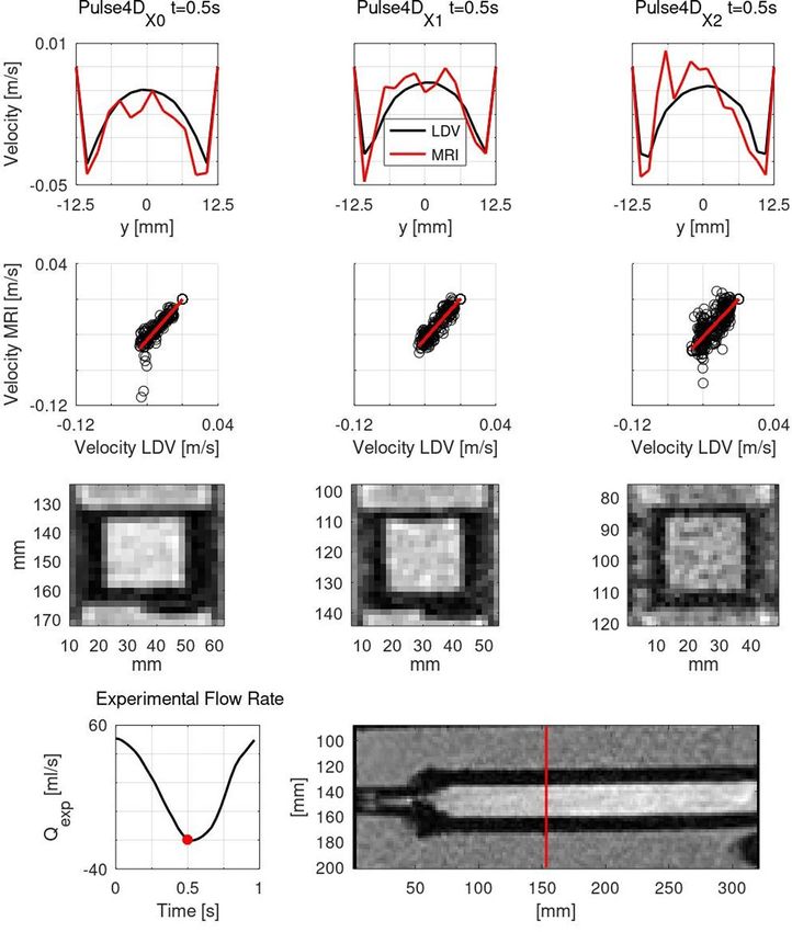
www.nature.com/scientificreports/
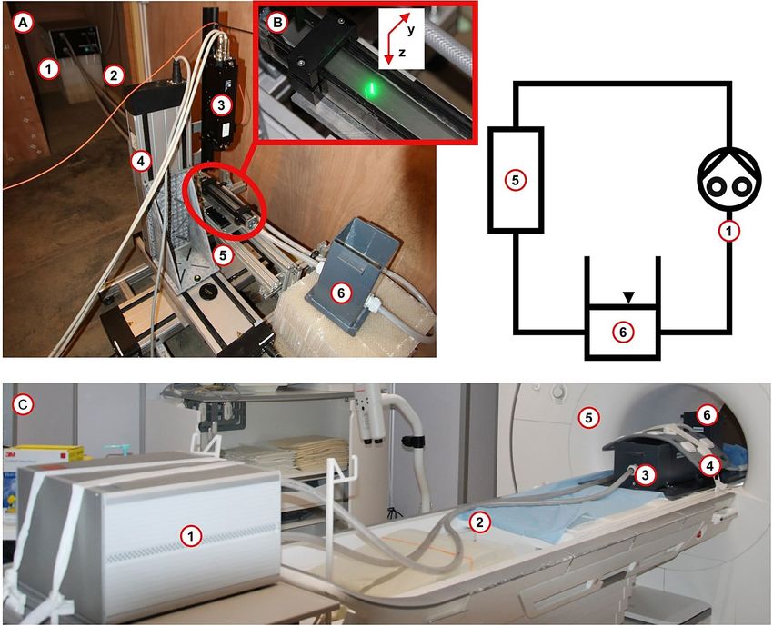
Figure 1. (a) Experimental set-up in LDV facility and its schematic (top, right): (1) Pulsatile Pump, (2)
Connecting pipes, (3) LDV head, (4) Laser displacement system, (5) Test Section, (6) Reservoir. (b) LDV
acquisitions. (c) Experimental Set-up in MRI facility: (1) Pulsatile Pump, (2) Connecting pipes, (3) Agarose gel
plastic box with the test section, (4) MRI array coils, (5) MRI system, (6) Reservoir.
(FEM) starting from a cubic interpolation of the velocity field on the nodes of a 3D mesh based on MRI voxels.
Finally, Piatti et al.13 developed an innovative method to compute WSS based on 2D and 3D Sobel filters.
PC MRI-derived WSS calculation methods are often validated with Computational Fluid Dynamics (CFD)
techniques in realistic vascular geometries. Nevertheless, CFD employment is limited in complex physiological
conditions14. Alternatively, in Laser Doppler Velocimetry (LDV) campaigns, it is possible to reproduce the same
experimental conditions of in vitro PC MRI acquisitions in terms of geometry, flow rate, pressure, fluid viscos-
ity, and density, providing accurate velocity profiles to serve as a reference for PC MRI data. LDV enables an
accurate measurement of absolute velocity components on a single point with the drawback of having to move
the measurement volume to obtain velocity mapping, and it represents an intrinsic, robust velocimetry technique
since velocity data are obtained through robust statistical post-processing tools. In the scientific literature, few
works about LDV validation for PC MRI-derived WSS computation are reported. Bauer et al. 15 successfully
investigated WSS accuracy from PC MRI data with LDV in a simplified model of an aortic aneurysm, employing
in parallel CFD for direct comparison.
The present work aims to develop a robust method based on a hydraulic circuit, in which LDV served as a
standard for velocity measurements, to be employed as a reference to assess the accuracy of 2D PC and 4D Flow
MRI velocity acquisitions. This method is intended to be employed to evaluate any potential developments in
acquisition and flow quantification protocols, particularly for the calculation of WSS. Firstly, a hydraulic test rig
was designed and manufactured to be MRI-compatible and to allow accurate LDV measurements under both
steady and pulsatile flow conditions. Next, velocity data obtained with the test rig were statistically analyzed to
assess the accuracy and reproducibility of results between the two velocimetry techniques. The correspondence
between LDV and PC MRI WSS profiles was statistically assessed. Finally, the efficacy of the method developed
in this work was tested evaluating the influence of 4D Flow MRI spatial resolution on WSS profiles.
Methods
Experimental set‑up. The experimental set-up (Fig. 1) was designed to keep limited dimensions, to be
easy to move between facilities, and to be compatible with LDV and MRI constraints. It was based on an MRI-
compatible gear pump (CardioFlow 5000, Shelley Medical Technology), a test section and a reservoir open to the
Scientific Reports | (2021) 11:4112 | https://doi.org/10.1038/s41598-021-83633-y 2
Vol:.(1234567890)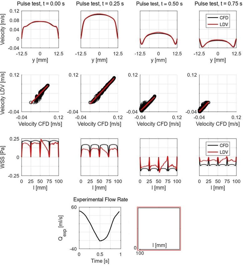
www.nature.com/scientificreports/
Experimental campaign 1 Experimental campaign 2: spatial resolution refinement
2D PC MRI 4D flow MRI 4D flow MRI
Test → Steady2DX0 Pulse2DX0 Steady4DX0 Pulse4DX0 Steady4DX1 Pulse4DX1 Steady4DX2 Pulse4DX2
Resolution
1.17 × 1.17 2.22 × 2.22 1.86 × 1.86 1.5 × 1.5
(mm)
Slice 1 32 32
Thickness
6 2 1.86 1.5
(mm)
Flip angle ( ◦) 20 7 7
Excitations 1 1
Averages 1 1
Gating R/P R/P
Phases 30 30
FOV (mm) 159 × 300 288 × 319 238 × 268 192 × 216
Matrix (px) 136 × 256 32 × 130 × 144 32 × 128 × 144 32 × 128 × 144
VENC (cm/s) 30 16 30 16 30 16 30 16
TE (ms) 3.73 4.72 3.49 4.28 3.53 4.31 3.57 4.36
TR (ms) 48.16 56.08 48.32 54.64 48.72 54.96 49.04 55.36
TA (min:s) 0:44 6:48 6:53 7.11
Temp Res (ms) 200 250 250
Table 1. Left: Standard 2D and 4D PC MRI experimental protocols. Right: Spatial resolution refinement 4D
PC MRI protocol. X0 original data resolution, X1 data resolution refinement 1, X2 data resolution refinement
2. Resolution refers to z–y axes and matrix refers to the number of pixels along z, y, and x axis respectively; see
Fig. 1b for axis reference. R/P retro/pulse, TE echo time, TR repetition time, TA acquisition time, Temp Res,
temporal resolution.
atmospheric pressure (Fig. 1a), completed with several connecting flexible PVC pipes for ease of assembly and
transport between LDV and MRI facilities. The pump provided a TTL signal to synchronize both LDV and MRI
acquisitions, the period of flow rate signals was Tc = 1 s for both steady and pulse acquisitions. Made of a mixture
of 40% by weight of glycerol in water, the working fluid reproduced blood density (ρ = 1098 kg/m3) and viscosity
(µ = 0.00345 Pa·s) closely16. The test section was a compact 25 × 25 × 345 mm squared PMMA pipe (Fig. 1b).
The measurement area was located on a cross-section placed 265 mm downstream of the test section inlet, to
limit the influence of the test section inlet and outlet. Investigations were performed under laminar steady and
pulse flow conditions, deploying an ultrasound flowmeter (Flowmax 44i, MIB Gmbh) to ensure the flow rate
control in the measurement location, Qexp (Qexp = 98.67 ml/s and Qexp = 16.47 + 35.64 sin (2πt + 0.50) ml/s
for steady and pulse flow rate respectively). During MRI measurements, a plastic box filled with agarose gel
(A8963, Applichem) surrounded the test section to reproduce human body tissues and to reduce noises (Fig. 1c).
Phase contrast MRI. Firstly, one standard 2D PC and one standard 4D Flow MRI sequence were used on
a 1.5 T MRI system (Aera 1.5T, Siemens), their parameters were selected as in current clinical practice, defin-
ing then tests called Steady2DX0, Pulse2DX0, Steady4DX0, and Pulse4DX0 (Table 1)17. In view to fit the maxi-
mum expected velocity vmax , the Velocity ENCoding (VENC) was adjusted as in Eq. (1) (vmax = 28 cm/s and
vmax = 12 cm/s for steady and pulse tests respectively).
vmax + 10%vmax for steady tests
VENC ≈
vmax + 30%vmax for pulse tests (1)
Next, a second experimental campaign was performed employing the 4D Flow sequence. The size of the voxels
was progressively reduced from 2.22 × 2.22 × 2 to 1.86 × 1.86 × 1.86, and then to 1.50 × 1.50 × 1.50 mm. The
refinement was carried out with isometric voxels to simplify the analysis; the starting size was considered as
“almost” isometric since the smallest dimension was shorter than the others by about 10%. Consequently, the
Field of View (FOV) was proportionally scaled. Acquisition parameters are resumed in Table 1, defining instead
tests subsequently called Steady4DX1, Steady4DX2, Pulse4DX1, and Pulse4DX2. Markers on the experimental set-
up enabled the placement of the measurement location at the center of the MRI scanner, drastically reducing the
effects of the magnetic field inhomogeneities. The velocity signal from the static homogeneous region composed
by the agarose gel was exploited to define the impact of the velocity offset from magnetic field inhomogeneities
and noise. The distribution of this signal was a Gaussian with a non-zero mean and variance, representing the
phase offset and the velocity noise respectively. As a first approximation, the influence of the offset was con-
sidered negligible; its ratio with the mean of the velocity signal ( v fluid ) in the fluid domain was lower than 3%.
To evaluate the impact of noise on PC MRI acquisitions, Velocity to Noise Ratio (VNR) was defined as in Eq.
(2) (σ v gel is the variance of velocity noise in the agarose gel calculated as the standard deviation of the velocity
signal of pixels in the agarose gel).
Scientific Reports | (2021) 11:4112 | https://doi.org/10.1038/s41598-021-83633-y 3
Vol.:(0123456789)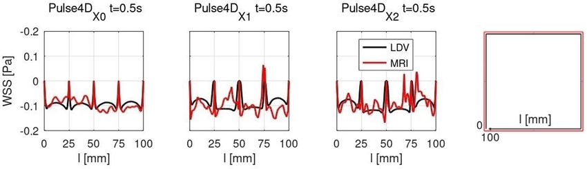
www.nature.com/scientificreports/
v fluid
VNR = (2)
σv gel
Laser doppler velocimetry. For LDV investigations, a low concentration (Cvolume ≈ 0.05 %) of 10 µm
silver-coated hollow glass spheres (S-HGS, Dantec) was added to the mixture. They exhibited a high refractive
index, increasing the LDV SNR with respect to non-coated hollow glass sphere seeding. The relative density
gap with the fluid (ρfluid /ρparticle ≈ 0.70) did not induce undesirable behaviors like a lift or gravitational effects,
particle accumulation, or modifications of the working fluid physical properties. The axial velocity along the
x-axis (see Fig. 1b for axes reference) was measured by an LDV system (fp50 LDV system). The optical path of
the laser beams passing through the upper face of the test section and the fluid was defined according to Snell’s
refraction law (Fig. 1b) (Eq. 3, α represents the incidence, in the air, or refraction, in the fluid, angle, and n the
refractive index).
nair sin αair = nfluid sin αfluid (3)
The location of a measurement point was calculated considering the refractive index mismatch at the opti-
cal interface along the z-direction, discounting the window thickness. To optimize the whole acquisition time,
measurements were obtained on a square grid of 63 × 63 points equally spaced by 0.40 mm; this length was the
LDV data spatial resolution. For each measurement point, the velocity was recorded for 30 s and velocity data
were obtained with a home-made Matlab script (Matlab R2016b, MathWorks). For steady tests, a two-class Gauss-
ian Mixture Model was applied to the velocity sample distribution to separate the signal Gaussian distribution,
determining the mean velocity and measurement uncertainty σs, from velocity outliers, determined during zero
flow rate measurements. For pulse acquisitions, the velocity signal was sampled in periods as long as those of the
pump flow rate; all periods were overlapped and finally fitted with a sinusoid, according to the Womersley theory
of velocity profiles under pulse flow conditions, for which velocity at each point has the same waveform of the
inlet flow rate18. The coefficient of determination R2 (best fit for R2 = 1) was employed to assess the uncertainty
of the measurement. A CFD verification study was performed to preliminary control LDV measured velocity
profiles on a simple test case for which CFD is deemed reliable. Numerical simulations were performed using
the Finite Volume Method (Star CCM+, Siemens). Calculations were based on a Cartesian mesh of 1725000
0.5mm-size cubic elements and results were then linearly interpolated to fit the LDV grid (Matlab R2016b,
MathWorks) for direct comparison. For the Steady test, the mean value of σs was 6.63 × 10⁻⁴ m/s, while for the
Pulse test the mean value of R2 was 0.82. The Locally Weighted Scatterplot Smoothing (LOWESS) method (Matlab
R2016b, MathWorks) was applied to experimental data to find velocity profile boundaries, smooth noises, and
scale results in a uniform grid. Ultimately, a broader LDV grid was generated to approach a similar resolution
of MRI data to allow direct comparison, with the average of all LDV points contained in a window with the
identical size of one MRI pixel.
Wall shear stress calculation. WSS is defined as (4)
∂�v
WSS = µ (4)
∂n wall
where µ is the blood dynamic viscosity, v the blood velocity, and n the normal direction to the arterial wall. The
methods proposed by Stalder et al.10 (2D-WSS) and Potters et al.11 (3D-WSS) were employed to assess WSS from
PC MRI and LDV data-sets in the same location of the test section, in view to demonstrate the efficacy of this
experimental system to validate PC MRI post-processing algorithms for WSS computation. For 2D-WSS, from
2D PC or sliced 4D Flow MRI data, the lumen is contoured through B-splines and within this fluid domain,
the blood velocity profile is interpolated with B-splines from which its derivative is calculated. In the 3D-WSS
method instead, velocity derivatives are calculated on the 3D lumen segmentation from B-splines interpolation
of blood velocity profiles, exploiting only a fixed number of velocity points close to the boundary.
Both methods were tested independently of the lumen segmentation technique. The lumen segmentation
was obtained from the test section CAD (SolidWorks 2016, Dassault Systèmes) as an stl file overlapping the test
section fluid domain in the anatomy images. Markers on the TS permitted to obtain data from different datasets
at the same location. The obtained data were employed as inputs for 2D-WSS. 3D-WSS calculations need to be
performed from 3D data sets. For 4D acquisitions, such 3D data sets are readily available, but it is not the case
for the two dimensional LDV and 2D PC MRI measurements. Thus, for these two latter, 3D data sets were arti-
ficially built by duplicating the 2D measurements in several planes in the x-axis (see Fig. 1b for axes reference),
spaced by 2 mm as in the 4D data sets. For 4D Flow MRI data resolution refinement, WSS was calculated only
with the 3D-WSS method.
For the comparison between LDV and CFD, WSS was calculated with a first-order finite difference scheme
(Eq. 5, µ is the fluid viscosity, s the spatial resolution, vwall and vwall+1 the velocity at the boundary and at the
boundary nearest point, respectively).
vwall+1 − vwall
WSSFD = µ (5)
�s
Scientific Reports | (2021) 11:4112 | https://doi.org/10.1038/s41598-021-83633-y 4
Vol:.(1234567890)www.nature.com/scientificreports/
Correlation Consistency19
PCC ≤ 0.3 None −− ICC ≤ 0.5 Poor −−
0.3 < PCC ≤ 0.5 Weak − 0.5 < ICC ≤ 0.75 Moderate −
0.5 < PCC ≤ 0.7 Moderate + 0.75 < ICC ≤ 0.9 Good +
PCC > 0.7 Strong ++ ICC > 0.9 Excellent ++
Table 2. Statistical analysis: perfect correspondence values for correlation (by PCC) and consistency (by ICC)
scores.
Statistical analysis. Flow Rate (Q) and WSS contour mean ( WSS ) were firstly computed through the inte-
gration of velocity and WSS profiles. For PC MRI data, Q and WSS were calculated for each phase and then for
Steady test they were averaged. Flow rate errors were calculated against values provided by the flowmeter Qexp,
while for WSS they were calculated with LDV as reference (Eq. 6, s and p refer to Steady and Pulse test respec-
tively).
| QMRI/LDV − Qexp |
ǫQs = 100 %
Qexp
s | WSSMRI − WSSLDV |
ǫWSS = 100 %
WSSLDV
MRI/LDV exp (6)
30
p
(Q − Qi )2
ǫQ = 100
i=1
i 30 exp 2 %
i=1 (Qi )
30 MRI LDV
p
(WSS − WSSi )2
ǫWSS = 100
i=1
30 i LDV 2
%
i=1 (WSSi )
Linear regression Y = aX + b was performed for velocity and WSS profiles, X = [xi , . . . , xN ] and
Y = [yi , . . . , yN ] were respectively the N velocity points of LDV and PC MRI datasets. Coefficients a and b were
determined for the analysis. Additionally, Root Mean Square Error (RMSE), Coefficient of Determination R2,
and L2 norm error ǫL2 were included in the analysis (Eq. 7)
N
1
yi − xi 2
RMSE =
N xi
i=1
N
(yi − xi )2
R2 = 1 − i=1 (7)
N 2
i=1 (yi − y)
N 2
i=1 (yi − xi )
ǫL2 = 100 N %
2
i=1 (xi )
Correlation between different velocity or WSS data was assessed with the Pearson Correlation Coefficient
(PCC), while consistency was assessed with Intraclass Correlation Coefficient (ICC). Coefficients a and b, RMSE,
R2, ǫL2, PCC, and ICC were evaluated for each acquired phase and subsequently averaged over the 30 samples.
Their scores for the exact correspondence between diverse groups of data are reported in Table 2.
Results
Preliminary verification of LDV with CFD. Results of the LDV verification with CFD are displayed for
the pulse test in Fig. 2. Velocity profiles show a good agreement between LDV and CFD, as well as correlation
plots with regression lines. WSS profiles display significant discrepancies between CFD and LDV, as CFD did not
reproduce the exact same experimental conditions. Specifically, results for values of the boundary coordinate l
between 25 and 75 mm might suggest that an imperfect alignment of the flow at the experimental test section
inlet occurred.
PC MRI velocity profiles. Results for velocity data centerlines and correlation plots between LDV and PC
MRI are reported in Fig. 3 for Pulse4DX0, Pulse4DX1, and Pulse4DX2 tests (see Table 1 for test labels), while the
quantitative analysis is summarized in Table 3. The effect of the resolution refinement on the magnitude images
is displayed in Fig. 2. Even though the refinement improved the image resolution, for the fine resolution, overall
image quality decreased. There was globally a good agreement between LDV and PC MRI results. Both 2D PC
and 4D Flow MRI reproduced LDV velocity profiles well, and the same feature was found with the refinement
of the spatial resolution in 4D acquisitions. 2D PC MRI results were noisier than those of 4D Flow MRI. Noise
impacted more data close to the boundaries and at low flow rate phases, as evidenced by the velocity oscillations.
Concerning the quantitative analysis, the VNR was higher for 4D Flow than 2D PC MRI, and for steady than
Scientific Reports | (2021) 11:4112 | https://doi.org/10.1038/s41598-021-83633-y 5
Vol.:(0123456789)www.nature.com/scientificreports/
Figure 2. LDV verification with CFD for pulse test at different time frames. First row: Velocity centerlines;
Second row: Correlation plots with regression lines in red; Third row: Finite difference WSS profiles on the
test section boundaries expressed in Pa, results are plotted along the boundary coordinate l, 0 ≤ l ≤ 100 mm;
Fourth row: Flow rate (left) and schematic of the boundary coordinate l to plot WSS profiles (right).
pulse acquisitions. Moreover, it decreased with voxel refinement in both steady and pulse acquisitions. For pulse
acquisitions, flow rate errors were lower for 2D PC than 4D Flow MRI. While refining 4D Flow data resolution,
it decreased to values comparable to those of 2D PC MRI. Pulse4DX1 test recorded the most satisfactory perfor-
mance. For the other statistical parameters, 2D PC and 4D Flow MRI results registered similar scores. Specifi-
cally, the correlation and consistency between LDV and MRI data were strong and excellent for steady tests and
strong and good for pulse tests, for both MRI techniques. Results related to Steady4DX1, Steady4DX2, Pulse4DX1,
and Pulse4DX2 tests displayed similar figures to those of Steady4DX0 and Pulse4DX0 tests. Despite these small
figures, data resolution refinement improved the correspondence between LDV and MRI datasets. For these
results, the correlation and consistency between LDV and MRI data were strong and excellent respectively.
Scientific Reports | (2021) 11:4112 | https://doi.org/10.1038/s41598-021-83633-y 6
Vol:.(1234567890)www.nature.com/scientificreports/
Figure 3. PC MRI Velocity Profiles, columns from left to right: Pulse4DX0, Pulse4DX1, Pulse4DX2 tests. First
row: Velocity centerlines; Second row: Correlation plots with regression lines in red; Third row: Magnitude
images; Fourth row: Flow rate and location of measurement cross-section in the test section, marked with the
red line.
PC MRI wall shear stress. Results of the WSS assessment are reported in Fig. 4 and in Table 4. Profiles of
3D-WSS calculated from 4D Flow MRI data displayed generally a satisfactory agreement with those obtained
from LDV velocity data. The refinement of the voxel size introduced oscillations in 3D-WSS profiles, particularly
Scientific Reports | (2021) 11:4112 | https://doi.org/10.1038/s41598-021-83633-y 7
Vol.:(0123456789)www.nature.com/scientificreports/
2D PC MRI 4D Flow MRI 4D Flow MRI
Test → Steady2DX0 Pulse2DX0 Steady4DX0 Pulse4DX0 Steady4DX1 Steady4DX2 Pulse4DX1 Pulse4DX2
ǫQ [%] 0.93 9.34 8.96 16.33 0.50 0.51 10.61 14.09
VNR 2.27 1.28 16.39 8.88 8.84 5.99 3.86 3.10
a 1.02 1.05 0.95 0.93 0.99 1.01 0.99 1.00
b -0.008 -0.001 -0.008 -0.003 -0.004 -0.008 -0.001 -0.003
RMSE 0.029 0.018 0.028 0.012 0.022 0.027 0.006 0.011
R2 0.87 0.57 0.89 0.69 0.93 0.90 0.88 0.75
ǫL2 17.94 64.03 20.03 56.38 14.31 16.81 28.03 43.51
PCC 0.93 (++) 0.74 (++) 0.94 (++) 0.81 (++) 0.97 (++) 0.95 (++) 0.94 (++) 0.86 (++)
ICC 0.96 (++) 0.8 (+) 0.97 (++) 0.86 (+) 0.98 (++) 0.97 (++) 0.96 (++) 0.91 (++)
Table 3. Statistical analysis for velocity results. Left: Standard PC MRI protocol. Right: 4D Flow MRI data
resolution refinement protocol. X1 resolution refinement 1, X2 resolution refinement 2.
Figure 4. 3D-WSS profiles on the test section boundaries expressed in Pa, results are plotted along the
boundary coordinate l, 0 ≤ l ≤ 100 mm. Right: Schematic of the boundary coordinate l to plot WSS profiles.
2D-WSS 3D-WSS
Steady2DX0 Pulse2DX0 Steady4DX0 Pulse4DX0 Steady2DX0 Pulse2DX0 Steady4DX0 Pulse4DX0
ǫWSS [%] 22.76 19.84 70.67 109.70 2.62 7.33 0.83 15.90
a 0.70 0.84 0.40 0.06 0.99 0.96 0.91 0.79
b 0.022 -0.003 -0.001 0.006 0.010 0 0.027 0.002
RMSE 0.084 0.047 0.012 0.036 0.041 0.037 0.026 0.023
R2 0.39 0.20 0.016 0.030 0.76 0.37 0.88 0.48
ǫL2 34.35 82.72 74.19 201.95 13.85 50.77 9.00 41.58
PCC 0.63 (+) 0.42(-) 0.39(-) 0.035 (–) 0.87 (++) 0.58 (+) 0.94 (++) 0.65 (++)
ICC 0.77 (+) 0.47 (–) 0.55(-) 0.014 (–) 0.93 (++) 0.64(-) 0.97 (++) 0.74(-)
3D-WSS
Steady4DX1 Steady4DX2 Pulse4DX1 Pulse4DX2
ǫWSS [%] 5.80 3.64 13.45 28.10
a 0.82 0.98 0.70 0.52
b 0.061 0.011 0.013 0.007
RMSE 0.049 0.086 0.030 0.042
R2 0.75 0.58 0.44 0.24
ǫL2 20.01 31.16 47.87 70.58
PCC 0.87 (++) 0.76 (++) 0.63 (+) 0.40 (−)
ICC 0.93 (++) 0.84 (+) 0.74 (−) 0.49 (−−)
Table 4. Statistical analysis for 2D-WSS and 3D-WSS results. Top: Standard PC MRI protocol. Bottom: 4D
Flow MRI data resolution refinement protocol. X1 resolution refinement 1, X2 resolution refinement 2.
Scientific Reports | (2021) 11:4112 | https://doi.org/10.1038/s41598-021-83633-y 8
Vol:.(1234567890)www.nature.com/scientificreports/
for t ≥ 0.5Tc . Concerning WSS quantitative analysis, overall results for 2D-WSS were inconsistent, particularly
for 4D Flow acquisitions, for which figures of mean WSS errors increased importantly. Also, for Steady tests, cor-
relation and consistency were weak and moderate respectively, while for Pulse tests, there was no correlation and
consistency was poor. Results of 3D-WSS instead recorded better performances. Figures were in the same order
of magnitude for 2D PC and 4D Flow MRI, but the results of pulse acquisitions were slightly worse. For Steady
tests, correlation was strong and consistency excellent while, for Pulse tests, consistency was moderate and con-
sistency was good for 4D Flow and moderate for 2D PC MRI. For data resolution refinement, results registered
improved performances for steady tests, and scores worsened with the decrease of the voxel size. However, for
steady tests, consistency and correlation remained excellent and strong respectively.
Discussions
In this work, an easy-to-use and accurate LDV-based system to validate potential improvements in PC MRI
acquisitions and post-processing was designed and manufactured. The reliability of the system was preliminarily
assured through the successful assessment of LDV measurement accuracy and errors. The experimental campaign
was carried out proficiently, proving the efficacy of the employment of this sort of tool in research on clinical
applications of PC MRI. Despite it being time-consuming, LDV enabled accurate measurements of fluid veloc-
ity profiles, providing information to test preliminary PC MRI performances and thus flow quantification, as it
did for WSS calculation. Even though LDV and PC MRI campaigns were performed independently at different
times, on the same test rig but in separated facilities, a good level of reproducibility of the results with the two
different techniques was achieved for both velocity and WSS results. Accurate LDV tools represent, therefore, a
robust alternative to CFD to simply assess 4D Flow MRI quality. Although CFD is often employed as a reference
for PC MRI, its role of ground truth is not widely accepted in the scientific community.
For velocity profiles, results generally showed a strong correlation and an excellent consistency between
PC MRI and LDV, representing a strong basement for further investigations on post-processing algorithms, as
evidenced by statistical parameter scores. Firstly, a method was employed to degrade the LDV data resolution
to directly compare LDV and MRI velocity profiles, inducing a small distance shift dshift between LDV and MRI
grids, but without a noticeable effect on the analysis (dshiftmax = 0.2632 mm). No significant differences were
noticed between standard 2D and 4D acquisitions, except for flow rate errors that were greater for 4D Flow
MRI results since data resolution was lower. As largely discussed, validation of WSS calculation techniques with
this experimental set-up represents a crucial clinical aspect. To demonstrate that, the system was proved with
two algorithms to compute WSS from PC MRI data. WSS calculation from PC-MRI-based velocity data in this
specific application was positively accomplished. Even if in clinical practice PC MRI data processing includes
segmentation of anatomical images to obtain the domain in which blood flow quantification is performed, the
analysis was simplified by testing the methods independently of the segmentation technique. The improved accu-
racy of 3D-WSS and its greater performances and versatility compared to 2D-WSS have been properly assessed
thanks to this LDV based tool. For 3D-WSS, there were no significant differences between 2D PC and 4D Flow
MRI results, while 4D Flow 2D-WSS outcomes were more inaccurate than 2D PC 2D-WSS. This high sensitivity
of the 2D-WSS method to the velocity data resolution might be due to the employment of a squared geometry,
representing a sensitive case for B-spline interpolation for the corners of lumen contour.
Finally, a concrete application of this approach to solve a relevant clinical challenge in 4D Flow MRI acquisi-
tions and derived WSS calculation was investigated to additionally prove the benefit of relying on LDV reference
data to optimize 4D Flow MRI. The influence of voxel size on acquired velocity data and computed 3D-WSS was
successfully assessed. For velocity profiles, the agreement between LDV and 4D Flow in terms of flow rate errors,
consistency, and correlation globally improved with the data resolution refinement. For the finest data resolution
compared to the medium one, this agreement worsened though, which might be attributed to a higher velocity
noise consequently to the voxel size reduction. This would also explain why the agreement between LDV and
4D flow MRI worsens when refining the resolution for 3D-WSS profiles, which are more sensitive to noise than
velocity profiles. The impact of noise is stronger for low-velocity data, like those close to the boundaries with
which WSS is calculated. This might have resulted in a reduction of the accuracy of the WSS assessment caused
by a significant increase in noise while refining the spatial resolution.
It can be revealed from this experimental campaign that, as a general rule in clinical practice, for an equiva-
lent acquisition time there is a trade-off to be found between data spatial resolution and VNR, as noise has a
stronger impact on WSS calculation with respect to the velocity measurement. For potential clinical applications
of current WSS computation techniques, an MRI spatial resolution improved with respect to that of standard
protocols might not always imply a more accurate assessment of WSS, if VNR is highly degraded by an increase
of noise in the acquired data. In this study, the effects of the temporal resolution were not investigated, but the
system could additionally be employed to accomplish this task.
Limitations of the present study included the employment of an unphysiological scenario, in terms of test
section shape and flow rate conditions, and the background phase removal. The selection of a squared test sec-
tion did not represent a realistic anatomical geometry. Nevertheless, it represented a simple and optimal set
up for accurate LDV measurements, since the optical interface crossed by LDV laser beams is constituted of
a flat-screen, preventing then optical aberrations, which could instead arise from a curved surface. Therefore
this squared test section was well suited to investigate the WSS biomarker. The flow rate curves were selected
to reproduce the thoracic aorta fluid dynamic conditions in terms of Reynolds ( Remean ≈ 1100) and Womer-
sley ( α ≈ 20) numbers, compatibly with the experimental set-up constraints ( Remean = 1273 for Steady tests;
Remean = 190 and α = 18 for Pulse tests). These unphysiological flow rate conditions led to lower magnitudes
of WSS signals, which were thus harder to assess. Nonetheless, the proposed methodology is valid for the higher
WSS magnitude found in physiological flow rate conditions. Further experimental campaigns with a more
Scientific Reports | (2021) 11:4112 | https://doi.org/10.1038/s41598-021-83633-y 9
Vol.:(0123456789)www.nature.com/scientificreports/
realistic scenario of flow rate and vessel geometry could be performed, however, with this experimental device.
Concerning the unphysiological flow rate conditions, for steady tests, the approximate average fluid dynamic
conditions of the thoracic aorta were achieved. For pulse tests instead, through the Womersley number, only
the pulsatile features of blood flow of this specific cardiovascular location were replicated. In any case, even if
during pulse tests velocity magnitudes were far from physiological values, this represented a challenging scenario
for the assessment of WSS, since velocity gradients were lower than physiological values. Further experimental
campaigns with a more realistic scenario of flow rate and vessel geometry will be performed.
Lastly, preliminary PC MRI processing procedures to remove the effects of magnetic field inhomogeneities
and other artefacts are mandatory in clinical investigations, but in this specific application, they were not imple-
mented. Their effects were evaluated considering velocity data in the agarose gel surrounding the test section,
and they were considered negligible in a first approximation. This might be explained by the fact that in this
straightforward application the region of interest was located in the center of the scanner where magnetic fields
are more homogeneous, and the FOV was properly centered in this region. Notwithstanding no correction was
applied, results showed a good agreement with other experimental references (LDV, flowmeter), and WSS assess-
ment was properly conducted. In this first preliminary phase, this aspect was not considered crucial, but it will
be considered for any other further investigations involving this experimental set-up.
This work represents a strong foundation for future validation of novel developments for blood flow quan-
tification from PC MRI acquisitions. Particularly, the method based on laser Doppler velocimetry presented
here might provide reliable information about the accuracy, reproducibility, and applicability of the techniques
employed to calculate in vivo WSS from 4D Flow MRI data. Based on the findings of this work, future develop-
ments of the present study are represented by the design of a novel hydraulic rig under more realistic conditions
in terms of physiological and pathological anatomies, flow rates, and pressure. It could be employed as an inde-
pendent standard to validate 4D Flow MRI acquisition sequences and post-processing, particularly regarding
quantitative hemodynamic biomarkers for blood flow quantification, such as the wall shear stress, pulse wave
velocity, or pressure mapping.
Data availability
The datasets generated during and/or analysed during the current study are available in the following repository
https://drive.google.com/drive/folders/1mGXXfrQALE-QcAeyT63_z3LJ7KJzkc5n?usp=sharing.
Received: 3 June 2020; Accepted: 2 February 2021
References
1. Global Burden of Disease Study. Global, regional, and national life expectancy, all-cause mortality, and cause specific mortality for
249 causes of death, 1980–2015: A systematic analysis for the global burden of disease study 2015. Lancet 388, 1459–1544. https
://doi.org/10.1016/S0140-6736(16)31012-1 (2016).
2. Malek, A. M., Alper, S. I. & Izumo, S. Hemodynamic shear stress and its role in atherosclerosis. JAMA 282, 2035–2042. https://
doi.org/10.1001/jama.282.21.2035 (1990).
3. Wentzel, J. J. et al. Endothelial shear stress in the evolution of coronary atherosclerotic plaque and vascular remodelling: Current
understanding and remaining questions. Cardiovasc. Res. 96, 234–243. https://doi.org/10.1093/cvr/cvs217 (2012).
4. Sengupta, P. P. et al. Emerging trends in CV flow visualization. J. Am. Coll. Cardiol. 5, 305–316. https://doi.org/10.1016/j.
jcmg.2012.01.003 (2012).
5. Stankovic, Z., Allen, B. D., Garcia, J., Jarvis, K. B. & Markl, M. 4D flow imaging with MRI. Cardiovasc. Diagn. Ther. 4, 173–192.
https://doi.org/10.3978/j.issn.2223-3652.2014.01.02 (2014).
6. Box, F. M. A. et al. Reproducibility of Wall Shear Stress assessment with the paraboloid method in the internal carotid artery with
Velocity Encoded MRI in healthy young individuals. J. Magn. Reson. Imaging 26, 598–605. https://doi.org/10.1002/jmri.21086
(2007).
7. Masaryk, A. M., Frayne, R., Unal, O., Krupinski, E. & Strother, C. M. In vitro and in vivo comparison of three MR measurement
methods for calculating vascular shear stress in the internal carotid artery. Am. J. Neuroradiol. 20, 237–245 (1999).
8. Oshinski, J. N., Ku, D. N. & Pettigrew, R. I. Determination of Wall Shear Stress in the Aorta with the use of MR phase velocity
mapping. J. Magn. Reson. Imaging 26, 640–647. https://doi.org/10.1002/jmri.1880050605 (1995).
9. Oyre, S. et al. Accurate noninvasive quantitation of blood flow, cross-sectional lumen vessel area and wall shear stress by three
dimensional paraboloid modeling of magnetic resonance imaging velocity data. J. Am. Coll. Cardiol. 32, 128–34. https://doi.
org/10.1016/S0735-1097(98)00207-1 (1998).
10. Stalder, A. F. et al. Quantitative 2D and 3D phase contrast MRI: Optimized analysis of blood flow and vessel wall parameters.
Magn. Reson. Med. 60, 1218–1231. https://doi.org/10.1002/mrm.21778 (2008).
11. Potters, W. V., van Ooij, P., Marquering, H. A., vanBavel, E. & Nederveen, A. J. Volumetric arterial wall shear stress calculation
based on cine phase contrast MRI. J. Magn. Reson. Imaging. 41, 505–516. https://doi.org/10.1002/jmri.24560 (2015).
12. Sotelo, J. et al. 3D quantification of wall shear stress and oscillatory shear index using a Finite-Element Method in 3D CINE PC-
MRI data of the thoracic aorta. IEEE T. Med. Imag. 35, 1475–1487. https://doi.org/10.1109/TMI.2016.2517406 (2016).
13. Piatti, F. et al. Towards the improved quantification of in vivo abnormal wall shear stresses in BAV-affected patients from 4D-flow
imaging: Benchmarking and application to real data. J. Biomech. 50, 93–101. https: //doi.org/10.1016/j.jbiome ch.2016.11.044 (2017).
14. Glaßer, S., Lawonn, K., Hoffmann, T., Skalej, M. & Preim, B. Combined visualization of wall thickness and wall shear stress for the
evaluation of aneurysms. IEEE Trans. Vis. Comput. Graph. 20, 2506–2515. https://doi.org/10.1109/TVCG.2014.2346406 (2014).
15. Bauer, A. et al. Comparison of wall shear stress estimates obtained by laser Doppler velocimetry, magnetic resonance imaging and
numerical simulations. Exp. Fluids. https://doi.org/10.1007/s00348-019-2758-6 (2019).
16. Cheng, N. Formula for the viscosity of a Glycerol–Water mixture. Ind. Eng. Chem. Res. https://doi.org/10.1021/ie071349z (2008).
17. Dyverfeldt, P. et al. 4D flow cardiovascular magnetic resonance consensus statement. J. Cardiovasc. Magn. Reson. https://doi.
org/10.1186/s12968-015-0174-5 (2015).
18. Womersley, J. Method for the calculation of velocity, rate of flow and viscous drag in arteries when the pressure gradient is known.
J. Physiol. https://doi.org/10.1113/jphysiol.1955.sp005276 (1955).
19. Koo, T. K. & Li, M. Y. A guideline of selecting and reporting Intraclass Correlation Coefficients for reliability research. J. Chiropr.
Med. 15, 155–163. https://doi.org/10.1016/j.jcm.2016.02.012 (2016).
Scientific Reports | (2021) 11:4112 | https://doi.org/10.1038/s41598-021-83633-y 10
Vol:.(1234567890)www.nature.com/scientificreports/
Acknowledgements
This work has been supported by the Région Pays de la Loire Grant MRI-Quantif. Authors would like to thank
Jérémy Wais, Mathieu Weber, Stéphane Lambert, Jean-Luc Toularastel, Anne Levesque, and Arnaud Merrien
from LHEEA Lab of Centrale Nantes for the provided assistance with LDV and set-up assembling.
Author contributions
M.C.: methodology, software, validation, formal analysis, investigation, visualization, writing—original draft.
S.L.: software, validation, investigation. P.P.G., S.M.: formal analysis, writing—review and editing. J.M.R., F.B.:
methodology, investigation, formal analysis, writing—review and editing. J.I.: formal analysis, supervision,
writing—review and editing. J.M.S.: conceptualization, investigation, supervision, writing—review and editing.
D.L.T.: methodology, formal analysis, investigation, supervision, writing—review and editing.
Competing Interests
The authors declare no competing interests.
Additional information
Correspondence and requests for materials should be addressed to D.T.
Reprints and permissions information is available at www.nature.com/reprints.
Publisher’s note Springer Nature remains neutral with regard to jurisdictional claims in published maps and
institutional affiliations.
Open Access This article is licensed under a Creative Commons Attribution 4.0 International
License, which permits use, sharing, adaptation, distribution and reproduction in any medium or
format, as long as you give appropriate credit to the original author(s) and the source, provide a link to the
Creative Commons licence, and indicate if changes were made. The images or other third party material in this
article are included in the article’s Creative Commons licence, unless indicated otherwise in a credit line to the
material. If material is not included in the article’s Creative Commons licence and your intended use is not
permitted by statutory regulation or exceeds the permitted use, you will need to obtain permission directly from
the copyright holder. To view a copy of this licence, visit http://creativecommons.org/licenses/by/4.0/.
© The Author(s) 2021
Scientific Reports | (2021) 11:4112 | https://doi.org/10.1038/s41598-021-83633-y 11
Vol.:(0123456789)You can also read