Time Series Anomaly Detection Using Convolutional Neural Networks and Transfer Learning
←
→
Page content transcription
If your browser does not render page correctly, please read the page content below
Time Series Anomaly Detection Using Convolutional Neural Networks and
                                                                         Transfer Learning

                                                                                         Tailai Wen1 , Roy Keyes2
                                                                                              Arundo Analytics
                                                                                  {1 tailai.wen, 2 roy.keyes}@arundo.com
arXiv:1905.13628v1 [cs.LG] 31 May 2019

                                                                   Abstract                                 Wang et al., 2017; Yin et al., 2017]). There has been
                                                                                                            some research using CNN’s for time series tasks, primar-
                                              Time series anomaly detection plays a critical role           ily around sequence classification (e.g. [Zheng et al., 2014;
                                              in automated monitoring systems. Most previous                Yang et al., 2015; Cui et al., 2016; Rajpurkar et al., 2017]).
                                              deep learning efforts related to time series anomaly             We recognized that time series anomaly detection shares
                                              detection were based on recurrent neural networks             many common aspects with image segmentation. When a
                                              (RNN). In this paper, we propose a time series seg-           person visualizes a time series and selects the anomalous seg-
                                              mentation approach based on convolutional neural              ment, if present, the perceptual process is very similar to a
                                              networks (CNN) for anomaly detection. Moreover,               person looking at an image and marking a desired object. In
                                              we propose a transfer learning framework that pre-            this research, we created a CNN-based deep network for time
                                              trains a model on a large-scale synthetic univariate          series anomaly detection. In particular, we were inspired by a
                                              time series data set and then fine-tunes its weights          successful image segmentation network, U-Net, and applied
                                              on small-scale, univariate or multivariate data sets          a time series version of U-Net to detect anomalous segments
                                              with previously unseen classes of anomalies. For              in time series. As the limited occurrence of failures is a com-
                                              the multivariate case we introduce a novel network            mon blocker for anomaly detection in industrial IoT systems,
                                              architecture. The approach was tested on multiple             we also propose a transfer learning framework to resolve the
                                              synthetic and real data sets successfully.                    data sparsity issue, including a new architecture, MU-Net, for
                                                                                                            transferring a univariate base model to multivariate tasks.
                                         1   Introduction                                                      The remainder of this paper is organized as follows: Sec-
                                         Time series anomaly detection plays a critical role in auto-       tion 2 includes a review of related work. We provide details
                                         mated monitoring systems. It is an increasingly important          of applying U-Net for time series anomaly detection in Sec-
                                         topic today, because of its wider application in the context of    tion 3. Section 4 introduces the transfer learning framework
                                         the Internet of Things (IoT), especially in industrial environ-    and introduces the MU-Net architecture for multivariate time
                                         ments [Da Xu et al., 2014].                                        series anomaly detection. We provide experimental obser-
                                            Before the boom of deep learning in the early 2010s, most       vations in Section 5, and conclude with some discussion in
                                         time series anomaly detection efforts were based on tradi-         Section 6.
                                         tional time series analysis (e.g. [Abraham and Chuang, 1989;
                                         Bianco et al., 2001]), or on approaches to extract and repre-      2   Related Work
                                         sent time series properties (e.g. [Chan and Mahoney, 2005;         Our approach was influenced by recent successes of deep
                                         Keogh et al., 2005; Ringberg et al., 2007; Ahmed et al.,           learning for image segmentation. [Long et al., 2015] pro-
                                         2007]). Some machine learning techniques for multivariate          posed a fully convolutional network (FCN), where com-
                                         outlier detection were also widely applied to detect anoma-        mon convolutional architectures for image classification (e.g.
                                         lies in multivariate time series (e.g. [Breunig et al., 2000;      AlexNet, the VGG net, and GoogLeNet) are used as en-
                                         Schölkopf et al., 2001; Liu et al., 2008]), although they treat   coders, and counterpart deconvolution layers are used for up-
                                         data points independently and neglect temporal relationships.      sampling as decoders. U-Net [Ronneberger et al., 2015] im-
                                            In recent years, advances in deep learning have revolution-     proved upon the FCN architecture by introducing so-called
                                         alized many areas of data-driven modeling. Recurrent neural        skip channels between encoding layers and decoding layers
                                         networks (RNN) and convolutional neural networks (CNN)             into the architecture, so that high-level features and low-level
                                         are two major types of network architectures that enabled          features are concatenated to prevent information loss along
                                         these breakthroughs. RNN’s are generally applied to tempo-         deep sequential layers. This architecture was proven suc-
                                         ral sequence tasks, while CNN’s are typically the first choice     cessful when applied to segmentation of neuronal structures
                                         for image related tasks. For this reason, most previous deep       in electron microscopic images in the original paper. It was
                                         learning work on time series anomaly detection was based           subsequently applied to several other biomedical image seg-
                                         on RNN’s (e.g. [Malhotra et al., 2015; Kim et al., 2016;           mentation tasks (e.g. [Çiçek et al., 2016; Dalmış et al., 2017;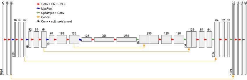
Figure 1: Architecture of U-Net for time series segmentation.

Dong et al., 2017]) as well as image segmentation prob-             This is followed by four decoding sections, where each sec-
lems in earth science (e.g. [Karchevskiy et al., 2018]), re-        tion includes an upsampling layer and two conv+BN+ReLu
mote sensing (e.g. [Yao et al., 2018]), and automated driving       blocks. The upsampling rate is also equal to 4, and the con-
(e.g. [Siam et al., 2017]).                                         volution layers uses the same number of filters as their coun-
   Our transfer learning work follows the success of deep           terpart encoding layers, making the architecture symmetric.
transfer learning in image and natural language processing.         An important feature of U-Net is the skip channels between
The design of synthetic pre-training data was in part inspired      corresponding encoding and decoding sections. This is im-
by [Mahajan et al., 2018]. Our fine-tuning strategies incorpo-      plemented by concatenating the output from every max pool-
rated some techniques presented in the Fast.AI courses1 .           ing layer with the output from the corresponding upsampling
   Data augmentation proved to be an important part of the          layer, and performing convolution over the concatenated fea-
research. Our time series augmentation strategies extended          ture series.
the previous work of [Um et al., 2017].                                The last section includes a convolution layer with a kernel
                                                                    size equal to 1 and an activation layer. Sometimes different
3       CNN-based Time Series Segmentation                          classes of anomalies are not mutually exclusive, and therefore
                                                                    the problem is a multi-class, multi-label problem, i.e. a time
We will introduce the details of how we build and train a time      point can be assigned to multiple classes. For example, a
series version of U-Net, including the detailed architecture,       spike on a periodic series is both an additive anomaly and a
how it is applied to streaming data in a production environ-        seasonal anomaly. In such a case, the number of filters at
ment, and some important issues, including input normaliza-         the final convolution layer is equal to the number of anomaly
tion and augmentation.                                              classes M , and the final activation function is a sigmoid so
                                                                    that probabilities of classes are independent. If all classes of
3.1       U-Net for time series segmentation                        anomaly are mutually exclusive, the output shape has depth
A time series can be regarded as a one-dimensional image            M + 1 and the additional column is for the nominal class
where the only dimension is temporal, whereas a typical im-         (i.e. no anomaly present). In this case, softmax activation is
age has two dimensions: width and height. A multivari-              applied so that the result is multi-class single-label. In both
ate time series may have an arbitrary number of channels,           cases, soft Dice loss is used as the loss function, as is the
which may have different properties and correlations with           case with many image segmentation networks, and the Adam
each other. In contrast, an image typically has only three          optimizer is used.
channels, RGB, and their properties and correlations are not
arbitrary. Following the design of U-Net, we propose the fol-       3.2    Prediction on Streaming Data
lowing architecture for time series segmentation as shown in        When deploying a trained model for production in a stream-
Figure 1. For a time series with length 1024 and C channels,        ing environment, we regularly take snapshots of the latest
it is encoded by five sections of convolution layers. Each sec-     batch of data and run the model on it. The frequency of taking
tion includes two layer blocks, each of which includes a con-       snapshots should be at least as high as the length of snapshot
volution layer, a batch normalization layer, and a ReLu layer.      so that every time point is evaluated by the model at least
For all convolution layers, the kernel size is equal to 3. The      once. We recommend using a frequency several times higher
number of filters in each convolution layer increases over the      than this minimal limit, and thus every time point is evalu-
five sections, from 16 to 256 by a factor of 2. For every con-      ated by the model a few times and we may ensemble multiple
volution layer, we apply zero padding and set the stride equal      results for the same time point to get more robust detection.
to 1. Between encoding sections, max pooling layers with a          Figure 2 shows an example where every data point is evalu-
pool size equal to 4 are used to downsample the feature series.     ated 3 times.
                                                                       Although the model input shape is fixed (e.g. 1024), it
    1
        https://www.fast.ai                                         is not necessary to always use it as the length of the snap-
to normalize the input series. Therefore, when applying the
model in production over snapshots, the detection will always
be based on the same scale. In some cases, the user does need
to detect anomalies only with respect to values inside a snap-
shot. The user may then add a sample-wise input normal-
ization layer at the start of the neural network, so that every
input snapshot is normalized independently and the scale will
be dynamic.
Figure 2: Anomaly detection on a data stream (top) by taking snap-
shots regularly and returning probability of anomaly (bottom). Figure 3: The same segment from a time series (top) in different
scales (middle and bottom).
shot. The length of the snapshot should be determined by
the streaming frequency and the time scale of anomalous be- 3.4 Augmentation
havior. If the streaming frequency is too high with respect
to anomalous behaviors, a long snapshot length (i.e. a large Data augmentation is a common approach to boost the size of
number of time points) should be used and every snapshot training data for robust models. [Um et al., 2017] introduced
needs to be downsampled to the model input size. If the a list of augmentation methods for time series, including time
streaming frequency is too low, a short length should be used warping, cropping, etc. We extended the list by adding a few
and upsampling is needed. methods, for example zooming, adding random trend, revers-
The strategy of sliding window could also work with a ing series, applying a random linear operation, random muta-
CNN-based classification model that classifies sequences by tion between multiple series, etc. These augmentation meth-
whether it includes anomalous subsequence. However, the ods were used during testing over different data sets.
choice of snapshot length would be problematic. If it is too As in image problems, augmentation of training data must
long, the localization of anomaly segments tends weak, since be label-invariant. In the context of anomaly detection, that
a snapshot is only classified by not segmented. On the other means an augmentation method must not change the nomi-
hand, if it is too short, the snapshot may not contain sufficient nality of a time series. Some augmentation operations are
context to distinguish itself from normal subsequence. The not label-invariant to certain types of anomaly. For exam-
proposed segmentation-based method, however, may over- ple, mutation operation may violate a periodic pattern when
come this difficulty by segmenting anomalous period in high applied to a seasonal series, so it should not be used to aug-
granularity. ment training data if the expected anomaly is an aberration of
a periodic pattern. Augmentation methods should always be
3.3 Input Normalization selected appropriately for the case under consideration.
Different from usual image problems, where values in a RGB
channel are always between 0 and 255, a time series may have
4 Transfer Learning
arbitrarily large or small values, and the magnitude scale may Sparsity of failure events in historical data often limits model
vary over channels. Figure 3 shows the same subsequence training in practice. Transfer learning is a strategy to resolve
from a stock price series in two different scales, where one the data sparsity issue. The transfer learning approach uses
looks essentially constant, while the other appears to have a the weights from a base model pretrained on an available
big jump. This is a common misleading issue, even when large-scale data set and then fine-tunes the model weights
a human views a time series. The proposed model requires with a small-scale data set related to the task of interest. The
a user to specify a magnitude scale first, and uses the scale hyper-parameter tuning process takes advantage of the modelpretrained on the large-scale data set, which tends to extract
useful features from the input, and therefore requires dramat-
ically less training data to converge without overfitting.
[Mahajan et al., 2018] explored factors that may impact
performance of transfer learning in CNN-based image pro-
cessing tasks. The similarity between the pretraining data set
and target data set has proven to be an important factor. The
correlation between pretraining task(s) and the target task also
plays a significant role. In our work, we define three pretrain-
ing tasks, i.e. three types of anomalies to detect, including
additive outliers, anomalous temporary changes of volatility,
and violations of cyclic patterns. These are the most common
types of anomalies found in univariate time series. Additive
outliers can be interpreted on a short time scale, violations
of cyclic patterns must be interpreted on a long time scale
that covers at least a few cycles, and changes of volatility
occurs on a medium time scale. We believe low-order fea-
tures representing these anomaly types are necessary compo-
nents to build higher-order features to represent more com-
plex anomalous behaviors. In other words, those features are
transferable to general the anomaly detection problem.
As features are not only extracted from anomalous seg-
ments, but also nominal segments, and thus, the nominal be-
havior of pretraining series should also be diverse. To pre-
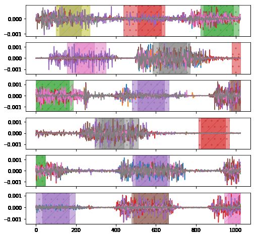
pare the pretraining data set, we generated a large number of Figure 4: Some samples from the pretraining data set with labelled
various synthetic time series, including smooth curves, piece- additive outliers (purple), changes of volatility (green), and viola-
wise linear curves, piece-wise constant curves, pulse-like sig- tions of cyclic patterns (red).
nals, etc. For each type, we generated some cyclic series and
some non-cyclic series. We augmented those time series by
cropping, jittering, adding random trends, and time warping, a different shape, as C is not equal to 1. If those kernels are
with different levels of intensity, such that the training data initialized randomly, then transferring weights of the deeper
covers a variety of nominal behaviors. We then adjusted ran- layers is meaningless, because the lowest-order features are
dom segments in these nominal series with the three previ- extracted differently. If we repeat the 3 × 1 × 16 weight ma-
ously mentioned types of anomalies to generate pretraining trix in the first layer of pretrained model C times and create
data with labelled anomalies. an initialization of the 3 × C × 16 weight matrix for the trans-
Figure 4 shows some examples from the pretraining data fer model, mathematically it is equivalent to extracting trans-
set. ferable features from the sum of all series channels. While
the sum of RGB channels may still maintain important prop-
4.1 Transfer Learning for Univariate Tasks erties from original images, the sum of time series channels
For transfer learning to another univariate task, we keep the is generally meaningless, for example, if the channels repre-
model architecture as in Figure 1, except that the output shape sent different sensors in an IoT system such as pressure and
of the final convolution layer must change according to the temperature.
number of classes in the target task. Weights of all layers We propose a new network architecture to transfer the
except the output section are initialized with weights from weights from a pretrained model as shown in Figure 5. Simi-
the pretrained model. We found two fine-tuning strategies lar to U-Net, this architecture also has an encoding-decoding
with good performance in our tests. The first one is to set up structure. However, the C channels of input series are sep-
different learning rate multipliers in 10 sections (5 encoding arated by a slicing layer first, and then every channel has its
sections, 4 decoding sections, and the output section) as 0.01, own univariate encoding sections, like the first four encod-
0.04, 0.09, ..., 0.81, 1.0. The other one is to freeze the weights ing sections in U-Net. The outputs from the fourth encoding
in the first two sections and only fine-tune the subsequent sec- section over all channels will be concatenated before an inte-
tions, and then to unfreeze the first sections and fine-tune all grated fifth encoding section, followed by four decoding sec-
weights. Both strategies returned similar results in our tests. tions and a final output section, the same as U-Net. We have
nicknamed this architecture MU-Net (multivariate U-Net).
4.2 MU-Net: A U-Net-based Network for Transfer When we transfer a pretrained U-Net model to a multivari-
Learning from Univariate to Multivariate ate task, we initialize weights in the first four encoding sec-
Tasks tions for every channel in MU-Net with the corresponding
When the pretrained base model is transferred to a multivari- weights in the pretrained model. During fine-tuning, we first
ate task, using the same U-Net architecture would be prob- freeze the first four encoding sections and tune the weights of
lematic. The kernel of the first convolution layer would have the remaining layers. We then unfreeze the third and fourthFigure 5: Architecture of MU-Net, a U-Net-based transfer network for multivariate tasks.
encoding sections and continue tuning. Finally we tune all
weights including the first two sections.
5 Experimental Evaluation
We tested the proposed approach in four scenarios: a univari-
ate task with sufficient data, a multivariate task with sufficient
data, a univariate task with insufficient data and transfer learn-
ing, and a multivariate task with insufficient data and transfer
learning.
All tests were conducted on an Nvidia GeForce GTX
1080Ti GPU. All implementation was done using Keras with
the TensorFlow backend.
Figure 6: Some snapshots in the Dodgers test case. Red markers
5.1 Dodgers Loop Sensor Data Set represent known events, green markers represent model detection.
This data set2 was originally introduced by [Ihler et al., 2006].
It includes a single time series of the traffic on a ramp close 5.2 Gasoil Plant Heating Loop Data Set
to Dodger Stadium over 28 weeks with 5-min frequency. The This data set3 was originally introduced by [Filonov et al.,
task is to detect anomalous traffic caused by sporting events. 2016]. It includes 48 simulated control sequences of a gasoil
There are a total of 81 known events. We use the first half of plant heating loop, which suffered cyber-attacks at some
the data (including 42 events) to train the model and the other points. All time series have 19 variables and an average
half (including 39 events) for testing. length of 204,615. We used the tag DANGER as the indi-
The training sequence was randomly cropped into 500 cator of attack events.
snapshots with lengths varying between 1,024 (about 3.5 We used 30 sequences for model training and the remain-
days) and 4,096 (about 2 weeks), and then downsampled to ing 18 for testing. The training data was randomly cropped
1,024. A univariate U-Net was created and trained. Only 3 into 300 snapshots with length 50,000, and then downsam-
known events out of 39 were not detected, and the missing pled to 1,024. A multivariate U-Net (C = 19) was created
detections were because these events were very close to pe- and trained. Among the 18 testing sequences with 22 cyber-
riods with many missing values. A few false positives also attacks in total (14 sequences with 1 attack, 4 with 2 attacks),
occurred, mostly near missing values. Figure 6 shows detec- only 1 attack was missed by detection. There were 3 false
tion results in some snapshots from the testing set. alarms.
2 3
https://archive.ics.uci.edu/ml/datasets/Dodgers+Loop+Sensor https://kas.pr/ics-research/dataset ghl 15.3 Synthetic Curves with Unusual Shapes because negative labels (i.e. segments with no gesture) are
We created a data set of synthetic curves where each series much less frequent than positive labels (i.e. segments with a
may have one or several segments with different curve shape gesture). However, since the approach we propose is funda-
from the rest of that series. For example, a series could be mentally a time series segmentation method, we believe this
mostly smooth except for a segment that is piece-wise linear. is still a good case for testing. This case is the only testing
We augmented the data set with several augmentation meth- case assuming a multi-class, single-label scenario, because
ods mentioned in Section 3.4, so that series behaviors are di- we know there was at most one gesture performed at a time
verse. We generated 1,400 samples with length 1,024: 700 point.
for training and 700 for testing. Figure 7 shows some exam- We trained a U-Net from scratch, and the IoU score eval-
ples. The task is to detect unusual segments, which is a more uated on the test set was 56.61%. We also trained an MU-
challenging task than the pretraining tasks. Although 700 is Net from scratch, and the IoU score was 64.10%. We then
larger than the size of data sets in the previous two testing transferred the pretrained U-Net to a MU-Net and fine-tuned
cases, it is still insufficient considering the diversity of time the weights, the IoU score then reached 70.04%. Figure 8
series behaviors over these samples. shows some testing snapshots with results from the trans-
We used intersection over union (IoU) score to evaluate ferred model.
the performance of this task. When training a U-Net from
scratch, the testing IoU was 50.96%. When we used univari-
ate transfer learning, the testing IoU reached 71.95%. Some
results from the transferred model are shown in Figure 7.
Figure 8: Some snapshots in the EMG test case. Dotted shadows
represent true segments, and striped shadows represent model seg-
ments. Different colors represent different gestures.
6 Conclusion and Discussion
In this work, we proposed a time series version of the con-
volutional U-Net for time series anomaly detection. As far
Figure 7: Some examples of synthetic curves with unusual shapes. as we are aware of, this is the first work to use a CNN-based
Red markers represent true anomalies, green markers represent deep network for time series segmentation in the context of
model detection. anomaly detection. The architecture was tested with both
univariate and multivariate examples and showed satisfactory
performance.
5.4 Electromyography (EMG) Data Set To address the challenge of data sparsity that often occurs
This data set4 was originally introduced by [Lobov et al., in real-world anomaly detection tasks, we proposed a trans-
2018]. It includes 8-channel myographic signals recorded by fer learning framework to transfer a U-Net model pretrained
bracelets worn on 36 subjects’ forearms. Each subject per- on a large-scale univariate time series set to general anomaly
formed the same set of seven gestures twice sequentially. The detection tasks. In particular, to transfer to a multivariate
task is to detect different gestures. Precisely speaking, this task, we proposed a new architecture, MU-Net, that may take
task is not an anomaly detection task but a segmentation one, advantage of the pretrained univariate U-Net. The transfer
learning framework was also tested with both univariate and
4
http://archive.ics.uci.edu/ml/datasets/EMG+data+for+gestures multivariate examples and returned promising results.One of the primary, inherent challenges in time series References
anomaly detection is defining ground truth. For time se- [Abraham and Chuang, 1989] Bovas Abraham and Alice
ries, delineating exactly when anomalous behavior occurs and Chuang. Outlier detection and time series modeling. Tech-
when it stops is a fundamental difficulty, as even human ex- nometrics, 31(2):241–248, 1989.
perts are likely to differ in their assessments. Additionally,
when detecting anomalies in time series, there is the question [Ahmed et al., 2007] Tarem Ahmed, Mark Coates, and
of what counts as a useful detection. For a typical image seg- Anukool Lakhina. Multivariate online anomaly detection
mentation task, the goal is to reproduce segmentation masks using kernel recursive least squares. In IEEE INFOCOM
as created by human labellers. For image tasks the level of 2007-26th IEEE International Conference on Computer
ambiguity is relatively low, i.e. edges are relatively well de- Communications, pages 625–633. IEEE, 2007.
fined. For time series anomaly detection, the predicted mask [Bianco et al., 2001] Ana Maria Bianco, M Garcia Ben,
and the ground truth mask may have less than perfect overlap, EJ Martinez, and Vı́ctor J Yohai. Outlier detection in re-
but, operationally, the predicted mask may still serve its pur- gression models with arima errors using robust estimates.
pose of alerting to the presence of a specific type of anomaly. Journal of Forecasting, 20(8):565–579, 2001.
Ultimately this means that the quantifying the goodness of [Breunig et al., 2000] Markus M Breunig, Hans-Peter
time series anomaly detection via segmentation is difficult. Kriegel, Raymond T Ng, and Jörg Sander. Lof: identify-
A transferable model is particularly well-suited for han- ing density-based local outliers. In ACM sigmod record,
dling the large variety of possible behaviors in time series volume 29, pages 93–104. ACM, 2000.
data. The pretraining dataset was populated with what we [Chan and Mahoney, 2005] Philip K Chan and Matthew V
considered to be the most fundamental anomalous behaviors
Mahoney. Modeling multiple time series for anomaly de-
in time series data. Because the definition of anomalous be-
tection. In Fifth IEEE International Conference on Data
havior is context-dependent, the pretraining dataset was de-
Mining (ICDM’05), pages 8–pp. IEEE, 2005.
signed to train a model capable of extracting informative, un-
derlying features for various types of time series and anoma- [Çiçek et al., 2016] Özgün Çiçek, Ahmed Abdulkadir, So-
lies, such that a new anomaly type may be easily learned from eren S Lienkamp, Thomas Brox, and Olaf Ronneberger.
a small-scale dataset. This methodology is fundamentally dif- 3d u-net: learning dense volumetric segmentation from
ferent from most previous work on anomaly detection, which sparse annotation. In International conference on medi-
were based on identifying outliers with an explicit or implicit cal image computing and computer-assisted intervention,
definition. While this scenario is less suited to handling pre- pages 424–432. Springer, 2016.
viously unseen anomalies than more traditional outlier detec- [Cui et al., 2016] Zhicheng Cui, Wenlin Chen, and Yixin
tion based methods, its strength lies in its robustness and abil- Chen. Multi-scale convolutional neural networks for time
ity to handle complex signals. series classification. arXiv preprint arXiv:1603.06995,
Future work on this topic could include extensive exper- 2016.
iments on factors that may impact transfer learning perfor- [Da Xu et al., 2014] Li Da Xu, Wu He, and Shancang Li. In-
mance, such as [Mahajan et al., 2018] performed for im- ternet of things in industries: A survey. IEEE Transactions
age classification. That paper explored, given specific target on industrial informatics, 10(4):2233–2243, 2014.
tasks, how a pretrained model may perform differently if it
was pretrained on ImageNet, or a certain part of ImageNet, [Dalmış et al., 2017] Mehmet Ufuk Dalmış, Geert Litjens,
or an even larger and more comprehensive data set. The cor- Katharina Holland, Arnaud Setio, Ritse Mann, Nico
relation between different types of time series (on both nom- Karssemeijer, and Albert Gubern-Mérida. Using deep
inal and anomalous behaviors) is even more subtle than that learning to segment breast and fibroglandular tissue in mri
between image classes. We believe that more research in this volumes. Medical physics, 44(2):533–546, 2017.
direction would help us improve the pretraining data set as [Dong et al., 2017] Hao Dong, Guang Yang, Fangde Liu,
well as the transfer learning framework, such that the pre- Yuanhan Mo, and Yike Guo. Automatic brain tumor de-
trained model would be even more transferable. tection and segmentation using u-net based fully convo-
Another area of possible future work is to create perfor- lutional networks. In annual conference on medical im-
mance comparisons with benchmark algorithms, such as sta- age understanding and analysis, pages 506–517. Springer,
tistical time series analysis, RNN-based anomaly detection 2017.
methods, and CNN-based classification methods with sliding [Filonov et al., 2016] Pavel Filonov, Andrey Lavrentyev,
windows. and Artem Vorontsov. Multivariate industrial time se-
ries with cyber-attack simulation: Fault detection us-
ing an lstm-based predictive data model. arXiv preprint
Acknowledgments arXiv:1612.06676, 2016.
[Ihler et al., 2006] Alexander Ihler, Jon Hutchins, and
We would like to thank Jason Hu and Gunny Liu for their Padhraic Smyth. Adaptive event detection with time-
help with synthetic data generation. We also thank Fausto varying poisson processes. In Proceedings of the 12th
Morales, Pushkar Kumar Jain, and Henry Lin for helpful dis- ACM SIGKDD international conference on Knowledge
cussions. discovery and data mining, pages 207–216. ACM, 2006.[Karchevskiy et al., 2018] Mikhail Karchevskiy, Insaf [Siam et al., 2017] Mennatullah Siam, Sara Elkerdawy, Mar-
Ashrapov, and Leonid Kozinkin. Automatic salt deposits tin Jagersand, and Senthil Yogamani. Deep semantic seg-
segmentation: A deep learning approach. arXiv preprint mentation for automated driving: Taxonomy, roadmap and
arXiv:1812.01429, 2018. challenges. In 2017 IEEE 20th International Conference
[Keogh et al., 2005] Eamonn Keogh, Jessica Lin, and Ada on Intelligent Transportation Systems (ITSC), pages 1–8.
IEEE, 2017.
Fu. Hot sax: Efficiently finding the most unusual time se-
ries subsequence. In Fifth IEEE International Conference [Um et al., 2017] Terry Taewoong Um, Franz Michael Josef
on Data Mining (ICDM’05), pages 8–pp. Ieee, 2005. Pfister, Daniel Pichler, Satoshi Endo, Muriel Lang, Sandra
Hirche, Urban Fietzek, and Dana Kulić. Data augmenta-
[Kim et al., 2016] Jihyun Kim, Jaehyun Kim, Huong Le Thi
tion of wearable sensor data for parkinson’s disease moni-
Thu, and Howon Kim. Long short term memory recur- toring using convolutional neural networks. arXiv preprint
rent neural network classifier for intrusion detection. In arXiv:1706.00527, 2017.
2016 International Conference on Platform Technology
and Service (PlatCon), pages 1–5. IEEE, 2016. [Wang et al., 2017] Zhiguang Wang, Weizhong Yan, and
Tim Oates. Time series classification from scratch with
[Liu et al., 2008] Fei Tony Liu, Kai Ming Ting, and Zhi-Hua deep neural networks: A strong baseline. In 2017 Interna-
Zhou. Isolation forest. In 2008 Eighth IEEE International tional joint conference on neural networks (IJCNN), pages
Conference on Data Mining, pages 413–422. IEEE, 2008. 1578–1585. IEEE, 2017.
[Lobov et al., 2018] Sergey Lobov, Nadia Krilova, Innoken- [Yang et al., 2015] Jianbo Yang, Minh Nhut Nguyen,
tiy Kastalskiy, Victor Kazantsev, and Valeri Makarov. La- Phyo Phyo San, Xiao Li Li, and Shonali Krishnaswamy.
tent factors limiting the performance of semg-interfaces. Deep convolutional neural networks on multichannel time
Sensors, 18(4):1122, 2018. series for human activity recognition. In Twenty-Fourth
[Long et al., 2015] Jonathan Long, Evan Shelhamer, and International Joint Conference on Artificial Intelligence,
Trevor Darrell. Fully convolutional networks for seman- 2015.
tic segmentation. In Proceedings of the IEEE conference [Yao et al., 2018] Wei Yao, Zhigang Zeng, Cheng Lian, and
on computer vision and pattern recognition, pages 3431– Huiming Tang. Pixel-wise regression using u-net and its
3440, 2015. application on pansharpening. Neurocomputing, 312:364–
[Mahajan et al., 2018] Dhruv Mahajan, Ross Girshick, Vig- 371, October 2018.
nesh Ramanathan, Kaiming He, Manohar Paluri, Yixuan [Yin et al., 2017] Chuanlong Yin, Yuefei Zhu, Jinlong Fei,
Li, Ashwin Bharambe, and Laurens van der Maaten. Ex- and Xinzheng He. A deep learning approach for intrusion
ploring the limits of weakly supervised pretraining. In Pro- detection using recurrent neural networks. Ieee Access,
ceedings of the European Conference on Computer Vision 5:21954–21961, 2017.
(ECCV), pages 181–196, 2018. [Zheng et al., 2014] Yi Zheng, Qi Liu, Enhong Chen, Yong
[Malhotra et al., 2015] Pankaj Malhotra, Lovekesh Vig, Ge, and J Leon Zhao. Time series classification using
Gautam Shroff, and Puneet Agarwal. Long short term multi-channels deep convolutional neural networks. In In-
memory networks for anomaly detection in time series. In ternational Conference on Web-Age Information Manage-
Proceedings, page 89. Presses universitaires de Louvain, ment, pages 298–310. Springer, 2014.
2015.
[Rajpurkar et al., 2017] Pranav Rajpurkar, Awni Y Hannun,
Masoumeh Haghpanahi, Codie Bourn, and Andrew Y Ng.
Cardiologist-level arrhythmia detection with convolutional
neural networks. arXiv preprint arXiv:1707.01836, 2017.
[Ringberg et al., 2007] Haakon Ringberg, Augustin Soule,
Jennifer Rexford, and Christophe Diot. Sensitivity of pca
for traffic anomaly detection. In ACM SIGMETRICS Per-
formance Evaluation Review, volume 35, pages 109–120.
ACM, 2007.
[Ronneberger et al., 2015] Olaf Ronneberger, Philipp Fis-
cher, and Thomas Brox. U-net: Convolutional networks
for biomedical image segmentation. In International
Conference on Medical image computing and computer-
assisted intervention, pages 234–241. Springer, 2015.
[Schölkopf et al., 2001] Bernhard Schölkopf, John C Platt,
John Shawe-Taylor, Alex J Smola, and Robert C
Williamson. Estimating the support of a high-dimensional
distribution. Neural computation, 13(7):1443–1471, 2001.You can also read