Feasibility of Load Shedding to Improve Efficiency and Reduce Energy Consumption on Passenger Locomotives, Phase I
←
→
Page content transcription
If your browser does not render page correctly, please read the page content below
0
 U.S. Department of
                        Feasibility of Load Shedding to Improve
                        Efficiency and Reduce Energy
 Transportation         Consumption on Passenger Locomotives,
 Federal Railroad       Phase I
 Administration

 Office of Research,
 Technology
 and Development
 Washington, DC 20590

DOT/FRA/ORD-20/29                                            Final Report
                                                             July 2020
NOTICE
This document is disseminated under the sponsorship of the
Department of Transportation in the interest of information
exchange. The United States Government assumes no liability for
its contents or use thereof. Any opinions, findings and conclusions,
or recommendations expressed in this material do not necessarily
reflect the views or policies of the United States Government, nor
does mention of trade names, commercial products, or organizations
imply endorsement by the United States Government. The United
States Government assumes no liability for the content or use of the
material contained in this document.
NOTICE
The United States Government does not endorse products or
manufacturers. Trade or manufacturers’ names appear herein solely
because they are considered essential to the objective of this report.REPORT DOCUMENTATION PAGE Form Approved
OMB No. 0704-0188
Public reporting burden for this collection of information is estimated to average 1 hour per response, including the time for reviewing instructions, searching existing data sources,
gathering and maintaining the data needed, and completing and reviewing the collection of information. Send comments regarding this burden estimate or any other aspect of this
collection of information, including suggestions for reducing this burden, to Washington Headquarters Services, Directorate for Information Operations and Reports, 1215 Jefferson
Davis Highway, Suite 1204, Arlington, VA 22202-4302, and to the Office of Management and Budget, Paperwork Reduction Project (0704-0188), Washington, DC 20503.
1. AGENCY USE ONLY (Leave blank) 2. REPORT DATE 3. REPORT TYPE AND DATES COVERED
Published July 2020 Technical Report
July 1, 2013–June 30, 2014
4. TITLE AND SUBTITLE 5. FUNDING NUMBERS
Feasibility of Load Shedding to Improve Efficiency and Reduce Energy Consumption on
Passenger Locomotives, Phase I DTFR53-12-D-00004 TO09
6. AUTHOR(S)
Anuradha Guntaka (0000-0003-1253-1127); Ken L. Martin (0000-0002-0346-3954); Som P.
Singh (0000-0002-6076-6839)
7. PERFORMING ORGANIZATION NAME(S) AND ADDRESS(ES) 8. PERFORMING ORGANIZATION
Sharma & Associates, Inc. REPORT NUMBER
100 W. Plainfield Rd
Countryside, IL 60525
9. SPONSORING/MONITORING AGENCY NAME(S) AND ADDRESS(ES) 10. SPONSORING/MONITORING
U.S. Department of Transportation AGENCY REPORT NUMBER
Federal Railroad Administration
Office of Research, Development and Technology DOT/FRA/ORD-20/29
Washington, DC 20590
11. SUPPLEMENTARY NOTES
COR: Melissa Shurland
12a. DISTRIBUTION/AVAILABILITY STATEMENT 12b. DISTRIBUTION CODE
This document is available to the public through the FRA website.
13. ABSTRACT (Maximum 200 words)
This report discusses the feasibility of temporarily shedding electrical demand associated with heating and ventilation air
conditioning (HVAC) systems of passenger cars during periods of peak traction, with the goal of right-sizing the main engine on a
passenger locomotive. Industrial approaches to load shedding were reviewed to evaluate whether they were suitable for
locomotive applications. Train simulations were conducted to determine the maximum time at peak traction when load shedding
would be required. Thermal simulations of a passenger coach were used to calculate the amount of time the coach interior would
stay within the temperature comfort zone if the HVAC was deactivated, which indicated that under most nominal conditions
deactivating HVAC systems during periods of peak traction would still lead to acceptable passenger comfort levels. Finally, an
economic analysis was conducted to estimate the benefit of load shedding, and it showed that an appropriate load shedding
strategy can be implemented without adversely impacting passenger comfort and the costs associated with a head end power
(HEP) system.
14. SUBJECT TERMS 15. NUMBER OF PAGES
Head end power, HEP, heating and ventilation air conditioning, HVAC, passenger car, load 36
shedding, locomotive, efficiency, heating and cooling, rolling stock 16. PRICE CODE
17. SECURITY CLASSIFICATION 18. SECURITY CLASSIFICATION 19. SECURITY CLASSIFICATION 20. LIMITATION OF ABSTRACT
OF REPORT OF THIS PAGE OF ABSTRACT
Unclassified Unclassified Unclassified
NSN 7540-01-280-5500 Standard Form 298 (Rev. 2-89)
Prescribed by
ANSI Std. 239-18
298-102
iMETRIC/ENGLISH CONVERSION FACTORS
ENGLISH TO METRIC METRIC TO ENGLISH
LENGTH (APPROXIMATE) LENGTH (APPROXIMATE)
1 inch (in) = 2.5 centimeters (cm) 1 millimeter (mm) = 0.04 inch (in)
1 foot (ft) = 30 centimeters (cm) 1 centimeter (cm) = 0.4 inch (in)
1 yard (yd) = 0.9 meter (m) 1 meter (m) = 3.3 feet (ft)
1 mile (mi) = 1.6 kilometers (km) 1 meter (m) = 1.1 yards (yd)
1 kilometer (km) = 0.6 mile (mi)
AREA (APPROXIMATE) AREA (APPROXIMATE)
1 square inch (sq in, in2) = 6.5 square centimeters (cm2) 1 square centimeter = 0.16 square inch (sq in, in2)
(cm2)
1 square foot (sq ft, ft2) = 0.09 square meter (m2) 1 square meter (m2) = 1.2 square yards (sq yd, yd2)
1 square yard (sq yd, yd ) 2
= 0.8 square meter (m ) 2
1 square kilometer (km2) = 0.4 square mile (sq mi, mi2)
1 square mile (sq mi, mi2) = 2.6 square kilometers (km2) 10,000 square meters = 1 hectare (ha) = 2.5 acres
(m2)
1 acre = 0.4 hectare (he) = 4,000 square meters (m2)
MASS - WEIGHT (APPROXIMATE) MASS - WEIGHT (APPROXIMATE)
1 ounce (oz) = 28 grams (gm) 1 gram (gm) = 0.036 ounce (oz)
1 pound (lb) = 0.45 kilogram (kg) 1 kilogram (kg) = 2.2 pounds (lb)
1 short ton = 2,000 pounds = 0.9 tonne (t) 1 tonne (t) = 1,000 kilograms (kg)
(lb) = 1.1 short tons
VOLUME (APPROXIMATE) VOLUME (APPROXIMATE)
1 teaspoon (tsp) = 5 milliliters (ml) 1 milliliter (ml) = 0.03 fluid ounce (fl oz)
1 tablespoon (tbsp) = 15 milliliters (ml) 1 liter (l) = 2.1 pints (pt)
1 fluid ounce (fl oz) = 30 milliliters (ml) 1 liter (l) = 1.06 quarts (qt)
1 cup (c) = 0.24 liter (l) 1 liter (l) = 0.26 gallon (gal)
1 pint (pt) = 0.47 liter (l)
1 quart (qt) = 0.96 liter (l)
1 gallon (gal) = 3.8 liters (l)
1 cubic foot (cu ft, ft3) = 0.03 cubic meter (m3) 1 cubic meter (m3) = 36 cubic feet (cu ft, ft3)
1 cubic yard (cu yd, yd ) 3
= 0.76 cubic meter (m ) 3
1 cubic meter (m3) = 1.3 cubic yards (cu yd, yd3)
TEMPERATURE (EXACT) TEMPERATURE (EXACT)
[(x-32)(5/9)] °F = y °C [(9/5) y + 32] °C = x °F
QUICK INCH - CENTIMETER LENGTH CONVERSION
0 1 2 3 4 5
Inches
Centimeters 0 1 2 3 4 5 6 7 8 9 10 11 12 13
QUICK FAHRENHEIT - CELSIUS TEMPERATURE CONVERSIO
°F -40° -22° -4° 14° 32° 50° 68° 86° 104° 122° 140° 158° 176° 194° 212°
°C -40° -30° -20° -10° 0° 10° 20° 30° 40° 50° 60° 70° 80° 90° 100°
For more exact and or other conversion factors, see NIST Miscellaneous Publication 286, Units of Weights and
Measures. Price $2.50 SD Catalog No. C13 10286 Updated 6/17/98
iiContents
Executive Summary .........................................................................................................................1
1. Introduction ..............................................................................................................................3
1.1 Background ....................................................................................................................... 3
1.2 Objectives .......................................................................................................................... 4
1.3 Overall Approach .............................................................................................................. 4
1.4 Scope ................................................................................................................................. 4
1.5 Organization of the Report ................................................................................................ 4
2. Research Methodology .............................................................................................................5
2.1 Load Shedding Approaches............................................................................................... 5
2.2 Determination of Peak Traction Requirements ................................................................. 6
2.3 Review of HVAC Compatibility with Load Shedding ................................................... 13
2.4 Passenger Coach Thermal Analysis ................................................................................ 14
2.5 Load Shedding Economic Analysis ................................................................................ 22
2.6 Barriers to Implementation .............................................................................................. 24
3. Conclusion ..............................................................................................................................26
3.1 Recommendations for Future Study ................................................................................ 26
4. References ..............................................................................................................................28
Abbreviations and Acronyms ........................................................................................................29
iiiIllustrations
Figure 2.1. Commuter route elevation profile, including the stops along the route ....................... 7
Figure 2.2. Commuter route speed limit locations .......................................................................... 7
Figure 2.3. Long-haul route elevation profile, including the stops along the route ........................ 8
Figure 2.4. Long-haul route speed limit profile .............................................................................. 9
Figure 2.5. Commuter route speed limit and simulated speed ...................................................... 10
Figure 2.6. Long-haul route speed limit and simulated speed ...................................................... 11
Figure 2.7. Isometric view of the bi-level passenger car .............................................................. 15
Figure 2.8. Isometric view of the car interior ............................................................................... 16
Figure 2.9. Representation of the interior air fluid nodes of the passenger car model in RadTherm
............................................................................................................................................... 16
Figure 2.10. Temperature mapping of car exterior obtained after 10 minutes of HVAC
deactivation simulation during winter at midnight (initial inside and outside temperature 72
°F and 20 °F, respectively) ................................................................................................... 17
Figure 2.11. Time to increase interior temperature out of comfort zone in cooling season with 74
°F initial interior temperature ............................................................................................... 19
Figure 2.12. Time to increase interior temperature out of comfort zone in cooling season with 72
°F initial interior temperature ............................................................................................... 20
Figure 2.13. Time to decrease interior temperature out of comfort zone in heating season with 74
°F initial interior temperature ............................................................................................... 20
Figure 2.14. Time to decrease interior temperature out of comfort zone in heating season with 74
°F initial interior temperature ............................................................................................... 21
ivTables
Table 2.1. Commuter train summary .............................................................................................. 8
Table 2.2. Long-haul train summary............................................................................................... 9
Table 2.3. Commuter maximum power time, outbound legs ....................................................... 12
Table 2.4. Commuter maximum power time, inbound legs ......................................................... 12
Table 2.5. Long-haul maximum power time, Midwest to California ........................................... 13
Table 2.6. Long-haul maximum power time, California to the Midwest ..................................... 13
Table 2.7. Overall dimensions of the passenger car ..................................................................... 17
Table 2.8. Time required to increase interior temperature outside comfort zone in cooling season
............................................................................................................................................... 21
Table 2.9. Time required to drop interior temperature outside comfort zone in heating season .. 22
Table 2.10. Economic Analysis Input Data .................................................................................. 23
Table 2.11. Comparison of NPV of cost-benefits for one HEP and one non-HEP train for 10-year
period .................................................................................................................................... 24
vExecutive Summary
Right-sizing a locomotive diesel engine for load demands on it (including traction and passenger
comfort) is beneficial from multiple perspectives. The Federal Railroad Administration (FRA)
sponsored Sharma & Associates, Inc. to conduct a study of whether a locomotive engine could
temporarily shed electrical demand associated with passenger car heating and ventilation air
conditioning (HVAC) systems during periods of peak traction, which would allow the main
engine to be right-sized, improving efficiency. The study was conducted from July 1, 2013, to
June 30, 2014, in Countryside, IL.
The project team determined that load shedding strategies are well-defined for industrial
applications but there are no methodologies for the rail environment, where the loads are not as
steady as industrial plants. No explicit strategy that directly applied to locomotives was found.
All load shedding approaches from other industry either automatically shut down systems to
reduce electrical demand quickly or requires personnel to shut down systems manually if a rapid
response is not needed. However, all the approaches discussed can be adapted for use in a
passenger rail environment.
As part of the project, passenger train operation simulations were conducted to determine the
length of time the locomotive operated at peak horsepower throttle over selected routes. For
low-powered equipment, it was determined that a locomotive could operate continuously in
notch 8 for as long as 10 consecutive minutes.
A finite element model of a typical bi-level passenger coach was analyzed under worst-case
cooling and heating conditions to determine the maximum length of time the HVAC system
could be deactivated and maintain the interior air temperature within the comfort bounds
(72–76 °F summer; 68–72 °F winter) of the Passenger Rail Investment and Improvement Act
(PRIIA) of 2008 passenger rail car specifications. The PRIIA established the Next Generation
Equipment Committee and tasked it with developing procurement specifications for standardized
next-generation intercity corridor equipment. The specifications for passenger comfort were used
as the benchmark for this effort. It was found that under worst-case conditions of extreme
exterior temperature the comfort bounds were exceeded after only 3 minutes with the HVAC
deactivated. However, this case is extreme and under typical weather conditions, the HVAC may
be shut-off for longer duration.
Next, an evaluation of the results of the train operation simulation, combined with thermal
analyses of a sample passenger car with the HVAC system occurred to surmise whether the
interior air temperature could be held within PRIIA comfort bounds during peak traction periods.
A brief economic analysis showed that there can be significant capital savings accrued by
avoiding installation of a separate HEP engine in a passenger locomotive. However, some of
these savings are offset by the additional control equipment required on the locomotive to
implement load shedding and maintain communication with the passenger coaches. In addition,
there are associated capital cost requirements on each passenger coach.
Finally, the team reviewed barriers to implementing passenger locomotive load shedding.
Equipment on both the locomotive and on the passenger coaches must be modified to implement
load shedding, while engineers must be trained appropriately and communication with
passengers must be established to make load shedding a successful strategy.
1Load shedding for passenger trains can be used to minimize capital and maintenance costs for
locomotives. Fuel savings that can be attributed to the elimination of HEP equipment weight are
too small to be reliably and accurately measured. Additional research is recommended to study
conceptual design for specific locomotive applications, as well as the validation of some of the
assumptions and results from this effort.
21. Introduction
From July 1, 2013, to June 30, 2014, Sharma & Associates, Inc. (SA), under sponsorship by the
Federal Railroad Administration (FRA), conducted research to study the feasibility of the
load-shedding concept to reduce electrical load on passenger locomotive prime mover engine
during moments of peak tractive effort. The project team research how load shedding is
implemented in other industry for possible adaptation to the rail industry.
1.1 Background
Traditionally, locomotives used in passenger service employ a separate engine to supply
electricity to power comfort features (e.g., heating and ventilation air conditioning [HVAC],
lighting, etc.) on the attached passenger coach consist. Commonly referred to as head end power
(HEP) or hotel power systems, these units generally consist of a diesel engine and associated
alternator that supplies 480 volts of alternating current (VAC), 3-phase (50-60 Hz) power. Some
variants have included systems where the HEP alternator is driven mechanically by the main
engine (i.e., prime mover), as well as some newer systems in which hotel power is taken from
the main alternator and conditioned using the appropriate power electronics to supply the
coaches.
In most conventional passenger locomotives, HEP output and demand is 600 to 700 hp and
newer locomotive specifications require even more HEP capacity. For example, the locomotive
specifications from the Passenger Rail Investment and Improvement Act (PRIIA) of 2008
requires 800 hp HEP. Even among modern higher speed/high horsepower locomotives, that is a
notable portion of the overall locomotive power output.
Some newer locomotives do not employ the traditional separate HEP model and instead use a
larger prime mover that supplies both traction and HEP needs. Combining the generation
capacity can address fuel efficiency concerns and the need to meet higher top speed requirements
with increased traction power. Additionally, the HEP engine will eventually need to meet U.S.
Environmental Protection Agency tier 4 emissions requirements, which will add to the overall
complexity of locomotive system design and packaging.
The horsepower needs of modern locomotives are driven by:
1. Traction requirements based on top speed, acceleration, trailing load, grades, etc.
2. HEP requirements based on the number of passenger coaches, heating/cooling
requirements, and passenger conveniences such as power ports, displays, WiFi, etc.
3. Auxiliary power for blower motors, radiator fans, control electronics, cab comfort, etc.
These demands are usually supplied by an auxiliary generator that is driven by the prime
mover. Auxiliary power requirements are generally lower than the much higher traction
and HEP power requirements (i.e., peaking at about 200 hp).
To accommodate the possibility of simultaneously satisfying the peak requirements of all three
sources, the locomotive might require a high capacity prime mover. In such a scenario, it is also
possible that under typical operations, the locomotive would rarely operate at full capacity under
typical operations, which means that this design will probably be sub-optimal. “Right-sizing” the
locomotive capacity of the prime-mover would be a better approach if one of the following
criteria applies:
3a. Peak traction, auxiliary, and HEP needs can be separated in time (i.e., temporal
separation of power peaks), such that peak requirements are unlikely to be simultaneous
b. HEP needs can be temporarily minimized, at times of peak traction demand, through an
automatic, controlled, load shedding process
1.2 Objectives
Whether either of the two criteria (i.e., temporal separation of peak power needs or load
shedding) is achievable depends on the type of passenger service under consideration (e.g.,
commuter, corridor, or long distance).
The project is divided into six major tasks:
1. Review existing load shedding strategies from other industries to determine if they would
be feasible in railroad passenger service
2. Determine peak traction requirements for commuter and long-distance trains with
appropriate simulations
3. Review HVAC technologies and determine if they are compatible with load shedding
4. Perform a thermal analysis of passenger coaches to determine the heat-up, or cool-down,
period after the HVAC is deactivated
5. Economic analysis of load shedding to evaluate the cost-benefit ratio
6. Review the barriers to implementing load shedding
1.3 Overall Approach
The intent of this project is to study the feasibility of load shedding with consideration of the
type of service, and to examine the technical, practical, reliability, and economic realities
surrounding specific techniques. This study only looks at load-shedding concepts as
implemented in other industries for possible implementation in the rail industry and does not
validate any particular concept for rail applications.
1.4 Scope
In performing tasks for this project, the research team investigated the feasibility of shedding
HVAC electrical demand loads during periods of peak traction requirements. An economic
analysis was conducted and showed that significant capital savings can be accrued by avoiding
installation of separate HEP.
1.5 Organization of the Report
This study is documented in the following sections:
Section 1 introduces the work and tasks that were performed to gain results from several
analyses.
Section 2 discusses the six major tasks conducted for this project.
Section 3 provides a summary of the purpose of the work and offers results that aid the
research team in presenting recommendations for future work.
42. Research Methodology
This section provides a detailed description for each of the six major tasks in this project.
2.1 Load Shedding Approaches
Industrial facilities use load shedding to manage situations when the demand for electrical power
is greater than the supply, whether self-generated or provided by an external source. When load
shedding is needed, some demand for electricity is temporarily removed in a controlled fashion
to avoid exceeding the current supply. Shedding electrical demand can occur when a facility
encounters capacity limitations, supply disturbances, or faces the need to save energy due to the
high costs of peak energy.
When a disturbance causes load shedding, the facility usually detects a drop in the supply
frequency—typically 100 Hz in an industrial plant—while load shedding to minimize usage
during peak power is usually done manually after the provider informs the facility that peak
power has begun.
Disturbances in electrical supply can be due to one or more of the following factors:
• Load generation capacity is strained
• Electrical and/or mechanical faults
• Complete or partial loss of power grid connection
• Complete or partial loss of on-site generation
• Length of disturbance and its termination (e.g., self-clearance, fault isolation, protection
device tripping, etc.)
• Subsequent system disturbances
• System frequency response (e.g., decay, rate-of change, final frequency)
• System voltage response (i.e., detected by frequency change that is caused by slow-down
of the generators)
• Operation of protective devices
• Power factor disturbance
During normal operation, the system load is equal to or less than the generated load. The system
is in a stable state and operates at a normal supply frequency. Slow load increases and minor
overloads are monitored by governors and will respond to the speed change, and unused capacity
will be used to equalize the system. Large rapid fluctuations in generation capacity impacts the
system resulting in a load imbalance and fast frequency decline.
There are a few different approaches to shedding the electrical load as outlined below.
Programmable Logic Controller
Most operations use a Programmable Logic Controller (PLC) installed on each electrical load
unit to control the load shedding process. The system is programmed based on system load vs.
generated load using maximum and minimum frequency conditions. The PLC’s are programmed
5to initiate a signal to trip the breaker. Breaker trips are done in a specific preset sequence to shed
the required load. This sequence continues until the frequency becomes normal and stable. Time
response between system detection and load shedding in larger systems is critical. In this system,
the load shedding is done in the same order every time unless the PLC's are reprogrammed for a
different sequence. The PLC reprogramming must be done locally, at each PLC.
Intelligent Logic Control
Intelligent logic control incorporates servers to continuously monitor and control the electrical
load. The server passes the trigger signal to the PLC to initiate the load shedding sequence. A
database of sequences of loads to be shed is compiled from all possible combinations, based on
various levels of power loss. Substantial time saving over only PLC control is achieved using
this technique since the server processing is faster than the PLC. Another benefit offered by
executing the required calculations at the server level is the ability to update load priority lists
and logic from one console. This reduces the downtime required for updating the logic and
eliminates removing and reprogramming the PLCs whenever a logic change has to be made.
There is usually a fail-safe or default priority table written to the PLCs which is used in the event
of server failure.
Interruptible Load Shedding
This approach is utilized mostly to avoid the high cost of electricity during peak demand times.
The utility will negotiate a contract with the high-demand industrial consumers to curtail usage
during peak demand times, typically in the summer months. The peak demand times may be
defined in the contract, or the utility may contact the consumer shortly before a peak demand
may occur. The consumer will then begin shedding loads using a scheme such as intelligent logic
control to meet the curtailed supply.
The passenger locomotive load application is most closely aligned with the interruptible load
shedding approach, since the goal is to shed loads only during times of peak demand, which
occur when maximum tractive effort is required.
2.2 Determination of Peak Traction Requirements
Determination of the peak traction requirements was conducted using FRA's Train Energy and
Dynamics Simulator (TEDS). This model simulates train operation given the track, train, and
train handling as inputs. A commuter route on the West Coast and a long-haul route between the
West Coast and major Midwest hubs were selected for simulation, with the goal of simulating
worst-case routes requiring the most tractive effort.
Once the train handling was determined, the TEDS simulator was run using this train handling to
accumulate both the total time spent operating in notch 8, as well as the single longest time
operated in notch 8.
2.2.1 Commuter Route
The commuter route includes 54 miles of track with a maximum grade of 3.0 percent. The route
included 11 stops. The simulation was conducted in both directions along the track to capture the
full extent of the grade variations. The elevation profile of the track in the outbound direction is
shown in Figure 2.1, along with the 11 stops with locations indicated by vertical red dashed
6lines. The speed limit profile in the outbound direction that provided the target speeds for the
train handling generator is shown in Figure 2.2.
Figure 2.1. Commuter route elevation profile, including the stops along the route
Figure 2.2. Commuter route speed limit locations
The train for this series of simulations includes one locomotive and six coaches. The train details
are summarized in Table 2.1. The locomotive power was determined by reviewing existing
passenger locomotive power capacity, and several locomotive models.
7Table 2.1. Commuter train summary
Locomotive power 2,400 hp
Locomotive weight 270,000 lb.
Number of coaches 6
Weight per coach (empty) 128,000 lb.
Weight per coach (loaded) 166,500 lb.
Total train weight 634.5 tons
Trailing weight 499.5 tons
Train length 569 feet
Horsepower per trailing ton 4.80
2.2.2 Long-Haul Route
The long-haul passenger route includes 54 miles of track with a maximum grade of 3.5 percent.
The route included 10 stops. The simulation was conducted in both directions along the track to
capture the full extent of the grade variations. The elevation profile of the track starting at the
Midwest hub is shown in Figure 2.3, along with the stops shown as vertical red dashed lines. The
speed limit profile starting at the Midwest that provided the target speeds for the train handling
generator is shown in Figure 2.4.
Figure 2.3. Long-haul route elevation profile, including the stops along the route
8Figure 2.4. Long-haul route speed limit profile
The train for the long-haul series of simulations includes two locomotives and eight coaches. The
train details are summarized in Table 2.2. The locomotive power was determined by reviewing
existing passenger locomotive power capacity, using several models.
Table 2.2. Long-haul train summary
Locomotive power 2,400 hp each
4,800 hp total
Locomotive weight 270,000 lb.
Number of coaches 8
Weight per coach (empty) 128,000 lb.
Weight per coach (loaded) 166,500 lb.
Total train weight 936 tons
Trailing weight 666 tons
Train length 798 feet
Horsepower per trailing ton 7.21
2.2.3 Train Simulation Summary
The makeup of both trains, which is typical of passenger train makeup, shows that the power to
weight ratio (hp per ton) is much greater than is typically present on the freight train, which is of
9the order of 2 hp per ton, or even less. Therefore, it is expected that the locomotives would not
require significant operation at full throttle to reach the track speed limit.
A comparison of the track chart speed limit and the speed achieved using the train handling
generator is shown in Figure 2.5 for the commuter rail operations simulation, and in Figure 2.6
for long-haul operations simulation.
Figure 2.5. Commuter route speed limit and simulated speed
10Figure 2.6. Long-haul route speed limit and simulated speed
The amount of time the locomotives were operating at maximum power was accumulated for
each of the legs. This is summarized in Table 2.3 through Table 2.6. Only a few of the legs
required operation at notch 8. The maximum continuous time spent in notch 8 was 10.2 minutes
in Leg 4 of the outbound commuter simulations. This leg includes a long ascending grade
averaging around 1 percent, which is a section of track on which the extended notch 8 operation
occurred. It is also important to note that the outbound and inbound legs are numbered from their
respective starting location. Therefore, outbound commuter Leg 1 is operated over the same
section of track as inbound commuter Leg 11. The time required to run over each segment is
different when the train is operated in the opposite direction since all the grades are reversed.
The results shown in Table 2.3 through Table 2.6 are for current, lower-powered locomotives. If
newer higher-powered locomotives are used to move the train, the maximum time spent in notch
8 reduces significantly. For example, the 10.2 minutes notch 8 time drops to half a minute for a
3,700 hp locomotive pulling the commuter train determined from a simulation of only Leg 4 (the
worst-case leg). The next-longest notch 8 duration is for the fifth leg of the long-haul route, and
this time would also drop significantly.
11Table 2.3. Commuter maximum power time, outbound legs
Commuter Longest notch 8 Total notch 8 Total
Leg time, minutes time, minutes simulation
time, minutes
1 0.0 0.0 8.7
2 0.0 0.0 22.8
3 0.0 0.0 13.9
4 10.2 12.8 19.4
5 0.0 0.0 6.7
6 1.2 1.2 11.4
7 0.0 0.0 11.4
8 0.0 0.0 5.5
9 0.0 0.0 6.4
10 0.0 0.0 16.1
11 0.1 0.3 17.1
Table 2.4. Commuter maximum power time, inbound legs
Commuter Longest notch 8 Total notch 8 Total simulation
Leg time, minutes time, minutes time, minutes
1 0.0 0.0 8.0
2 0.0 0.0 7.0
3 0.0 0.0 5.3
4 0.0 0.0 5.2
5 1.5 1.5 7.2
6 0.0 0.0 13.5
7 0.0 0.0 13.5
8 0.0 0.0 19.5
9 0.0 0.0 21.1
10 1.8 1.8 16.9
11 0.0 0.0 8.8
12Table 2.5. Long-haul maximum power time, Midwest to California
Leg Longest notch 8 time, Total notch 8 Total simulation
minutes time, minutes time, minutes
1 0.0 0.0 154.9
2 0.0 0.0 238.7
3 1.5 1.5 297.6
4 0.0 0.0 274.3
5 0.0 0.0 229.8
6 0.0 0.0 620.7
7 0.0 0.0 686.9
8 0.0 0.0 653.4
9 0.0 0.0 767.4
10 0.0 0.0 1,226.9
Table 2.6. Long-haul maximum power time, California to the Midwest
Leg Longest notch 8 Total notch 8 Total simulation
time, minutes time, minutes time, minutes
1 0.0 0.0 765.7
2 0.0 0.0 874.5
3 1.5 1.5 825.4
4 0.0 0.0 502.8
5 3.6 4.8 653.3
6 0.0 0.0 543.3
7 0.0 0.0 452.8
8 0.0 0.0 294.4
9 0.0 0.0 233.6
10 0.0 0.0 167.0
2.3 Review of HVAC Compatibility with Load Shedding
Implementation of load shedding in a passenger train requires that the HVAC equipment be
suitable for remote shutdown. This approach is comparable to electric utilities offering
residential customers the option of electricity rate reduction by having the air conditioner
remotely turned off for brief periods during high-demand times. The utility manages the remote
shut off device.
13Air conditioners typically require a few minutes of down time after shutdown before the system
can be restarted. Modern thermostats have the timer built into the logic of the programming.
Technically there is no difference between the thermostat deactivating the HVAC and a remote
unit deactivating the HVAC. The only requirement is that the system restart timer be activated
when the remote shut off is in effect.
Some additional communications between the passenger coaches and the locomotive are
required to facilitate load shedding. First, the locomotive must be able to initiate the HVAC shut
off, and communicate when HVAC systems can be restarted when the engineer has moved out of
notch 8. Second, the passenger coaches must be able to communicate to the locomotive when the
interior temperature has exceeded the comfort bounds, therefore, the HVAC system must be
reactivated. In this case the locomotive may need to be moved out of notch 8 before the engineer
would have normally done so.
2.4 Passenger Coach Thermal Analysis
Temporarily deactivating the HVAC inside passenger coaches to obtain maximum traction on
the locomotives may result in the interior temperature of the passenger coaches to move into a
range of discomfort.
It is the objective of this task to evaluate the effect of HVAC system deactivation on the
passenger comfort.
The PRIIA specifications for passenger coaches include provisions for passenger comfort. These
specifications include allowable temperature variations of [1]:
1. Vertical (same floor) [5 °F maximum]
2. Horizontal [±3 °F from the average temperature at that level]
3. Top level to bottom level [4 °F maximum]
4. Seasonal conditions [72–76 °F summer; 68–72 °F winter]
The seasonal conditions listed above are specified for ensuring that the design of the HVAC
system can maintain the interior temperature for both extremes of exterior conditions. Thus, they
account for the exterior conditions in the summer by adding heat to the coach, and during the
winter the exterior conditions remove heat from the coach. Therefore, in summer the coach
interior is typically warmer than in winter. Thus, an acceptable range of interior temperature is
the extremes from both seasons at 68–76 °F.
The comfort zone temperature variation given in the PRIIA document does not specify a location
at which the temperature is to be measured. Since the actual temperature variation allowed by
stacking up the ranges listed above can be greater than the 4 °F temperature design range of each
of the seasonal conditions, the researchers interpreted the specification to mean the average air
temperature within the passenger car should remain within the 68–76 °F range.
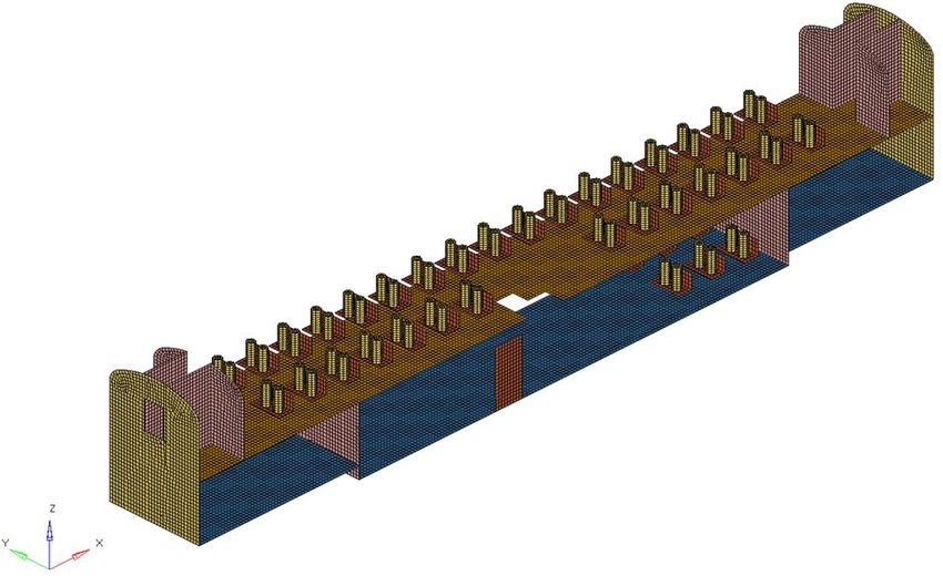
A bi-level passenger car was selected for this thermal analysis. The model included elements to
represent the car structure and seats as well as nodes for the interior air temperature. Passenger
heat loading for a full complement of 90 passengers was included in the analysis.
The geometric model of a long distance bi-level passenger car was created in HyperMesh and is
shown in Figure 2.7. The representation of passengers and seats inside the car is shown in
14Figure 2.8. This model was then imported into RadTherm, which is a thermal analysis program.
Air fluid nodes were added to the model to represent the interior air (shown in Figure 2.9). Only
the air temperature in the seating area compartments was considered in the evaluation.
The passenger car was simulated in both the heating and cooling conditions to determine the
time required for the average interior temperature to move out of the comfort specification.
Several exterior and interior condition combinations were analyzed.
Figure 2.7. Isometric view of the bi-level passenger car
15Figure 2.8. Isometric view of the car interior
Figure 2.9. Representation of the interior air fluid nodes of the passenger car model in
RadTherm
The overall dimensions of the passenger car are listed in Table 2.7.
16Table 2.7. Overall dimensions of the passenger car
Length (ft.) Width (ft.) Floor Height (each floor) (ft.)
82.5 10.0 7.1
The car exterior, the bottom floor, and the roof were modeled to include multiple layers of
materials incorporating a layer of insulation in the center.
Several cases were simulated for summer conditions, with both 72 °F and 74 °F initial inside
temperature and a range of outside ambient temperatures. The maximum ambient outside air
temperature for the summer was chosen as 110 °F since that condition is the HVAC system
design criteria defined in the PRIIA specification. The passenger car was simulated at noon on a
cloudless day for the worst-case incident solar radiation, which includes reflection into the coach
through the windows. A heating load of 74 seated passengers, with every seat occupied, was
included in the thermal model as a worst-case scenario. A period of 10-minutes was chosen for
simulation since that is the maximum time that the HVAC system would need to be shut off, as
determined from the train simulations discussed in Section 2.2, for the current locomotive power
output. Newer, more high-powered locomotives would only be required to operate in notch 8 for
only a few minutes.
The level of detail included in the carbody model is demonstrated in Figure 2.10, which shows
temperature mapping of the car exterior obtained after 10 minutes of HVAC deactivation with an
initial inside temperature of 72 °F and outside air temperature of 20 °F. The interior walls and
floor clearly show as hotter areas than the bare walls. The windows are also able to better
transfer heat, and are hotter on the outside than the exterior walls.
Figure 2.10. Temperature mapping of car exterior obtained after 10 minutes of HVAC
deactivation simulation during winter at midnight (initial inside and outside temperature
72 °F and 20 °F, respectively)
17The average interior air temperature variation within a 10-minute time period at noon is shown in
Figure 2.11 and Figure 2.12. The time it takes to cause the average interior temperature of the
passenger car to move outside the comfort range for all the summer cases was calculated and is
shown in Table 2.8. The minimum time for the passenger car interior to move outside the
comfort zone is 3.1 minutes as shown in Table 2.8 for the cooling season. This minimum time is
for the worst-case exterior condition of 110 °F air temperature. The time for the temperature to
exceed the upper comfort bound becomes longer both when the initial interior temperature is
lower and when the exterior temperature is lower.
Several cases were simulated for winter conditions, with both 72 °F and 74 °F initial inside
temperature and a range of outside ambient temperatures. The minimum outside air temperature
for winter was chosen as -30 °F since that condition is the HVAC system design criteria defined
in the PRIIA specification. The passenger car was simulated at midnight for the worst-case of no
incident solar radiation. A period of 10-minutes was chosen for simulation since that is the
maximum time that the HVAC system would need to be shut off, as determined from the train
simulations discussed in Section 2.2.
The average interior air temperature variation in a 10-minute time period at midnight is
illustrated in Figure 2.13 and Figure 2.14. Table 2.9 shows the time it takes to decrease the
average interior temperature of the passenger car outside the comfort range for all the winter
cases. The minimum time to drop the interior temperature is 3.6 minutes as shown in Table 2.9.
This minimum time is for the worst-case exterior condition of -30 °F air temperature. The time
for the temperature to exceed the upper comfort bound becomes longer both when the initial
interior temperature is lower and when the exterior temperature is lower.
The researchers investigated the relative contribution of each of the variables in the thermal
model to the time the average interior temperature remains in the comfort zone. The ranking of
the variables in descending order of impact is:
1. Heat load from passengers (2-minute increase in cooling season with no passengers)
2. Initial interior temperature when the HVAC system is deactivated (1 minute per 1 degree
drop)
3. Decreased speed leading to smaller heat transfer coefficient (less than 1 minute additional
time at zero speed)
4. Increased insulation layers (less than 1 minute additional time)
5. Effect of radiation from sun (less than 0.5-minute comparing noon to midnight)
For example, the time required for the interior temperature to exceed the comfort zone increases
by a factor of about 1.7 when the initial interior temperature is dropped by 2 °F in the cooling
season. This ratio drops to about 1.3 in the heating season when the initial interior temperature is
increased by 2 °F. The reason the change ratio is greater in the cooling season is because the
interior to exterior temperature difference is less than in the heating season. The temperature
difference across the carbody walls drives the heat transfer through the walls. A larger
temperature difference results in a larger heat transfer rate, so that the small change in initial
interior temperature does not as significantly change the time of the temperature drop.
Figure 2.11 and Figure 2.12 also show that if the interior temperature could be allowed to rise to
78 °F the time the HVAC system could be shut off increases by more than 2 minutes.
18The researchers conclude that a communication system must be integrated into the HVAC shut
off to inform the engineer when the throttle should be reduced from the maximum setting to
maintain passenger comfort. This communication system is required even if the comfort levels
can be maintained for the 10-minute maximum window since there could be other situations in
which the throttle might be maintained for longer than 10 minutes. The time the HVAC system
can be deactivated will be extended if one or more of the following can be done:
1. Expand the allowable interior temperature range
2. Increase the interior temperature set point during the heating season and decrease the
interior temperature set point during the cooling season
It is also possible to allow the interior temperature to slightly exceed these comfort boundaries.
For example, the 76 °F upper bound could be extended to 78 °F, which would increase the time
with the HVAC shut off by approximately 2.5 minutes.
The period of deactivation of the HVAC system is much less with new high-powered
locomotives. The length of time that the temperature stays within the comfort range is greater
than the period of notch 8 operation. Therefore, the newer equipment can likely sustain load
shedding much more easily.
Figure 2.11. Time to increase interior temperature out of comfort zone in cooling season
with 74 °F initial interior temperature
19Figure 2.12. Time to increase interior temperature out of comfort zone in cooling season
with 72 °F initial interior temperature
Figure 2.13. Time to decrease interior temperature out of comfort zone in heating season
with 74 °F initial interior temperature
20Figure 2.14. Time to decrease interior temperature out of comfort zone in heating season
with 74 °F initial interior temperature
Table 2.8. Time required to increase interior temperature outside comfort zone in cooling
season
Exterior
Time to move outside comfort range (minutes)
Temperature (°F)
72 °F Initial Interior Temp 74 °F Initial Interior Temp
90 7.5 4.3
100 6.0 3.5
110 5.2 3.1
21Table 2.9. Time required to drop interior temperature outside comfort zone in heating
season
Exterior
Time to move outside comfort range (minutes)
Temperature (°F)
72 °F Initial Interior Temp 74 °F Initial Interior Temp
-30 3.6 4.7
-20 3.9 5.1
-10 4.2 5.5
0 4.6 6.1
10 5.1 6.8
20 5.8 7.7
2.5 Load Shedding Economic Analysis
The economic analysis is based on one train (i.e., one locomotive, and six or eight cars). The
factors included in the analysis are:
1. Capital cost to install the HEP system (is this assuming that a new HEP is required that
can be regulated electronically for activation and deactivation? Does this include the net
costs associated with making the HEP ‘intelligent’ as in a retrofit scenario? Net cost
between convention and ‘intelligent’ HEP)
2. Maintenance cost of the HEP system
3. Estimated cost of electronics required to implement load shedding
4. Estimated maintenance cost of electronics for load shedding
5. Fuel savings due to reduced locomotive weight when the HEP system is not installed
6. Fuel savings due to load shedding
The data used as input to the economic model are shown in Table 2.10.
22Table 2.10. Economic Analysis Input Data
Parameter Cost
Estimated purchase cost of one high-speed PRIIA $7,000,000
compliant locomotive
Installation cost of the HEP system in one locomotive $700,000
Annual maintenance cost of one HEP system per year $800
Estimated installation cost of additional electronics in $10,000
locomotive to implement load shedding
Estimated annual maintenance cost of locomotive $700
load shedding electronics
Estimated installation cost of additional electronics in $60,000
six passenger coaches
Estimated annual maintenance cost of coach load $4,200
shedding electronics
Fuel cost savings due to drop in train resistance from $740
the weight decrease with no separate HEP system, per
year (assuming average speed of 25 mph)
Fuel cost savings due to load shedding per year $5,400
Net present value (NPV) discount rate 7%
The analysis was conducted for a 10-year period. It was assumed that the locomotive was
purchased at the start of the first year, and that all passenger coaches were modified at the start of
the first year.
The HEP maintenance cost includes labor and consumable items (e.g., filters and fluid sampling)
for the annual inspection, semiannual inspection, and two quarterly inspections.
The average price of diesel fuel was assumed to be $4.00/gallon.
The fuel savings due to weight decrease was calculated based on the resistance change at an
assumed 25 mph average speed. The procedure was to:
1. Calculate the locomotive resistance force with the HEP system (657.4 lb.)
2. Calculate the locomotive resistance force without the HEP system (650.1 lb.)
3. Calculate the savings in work done per mile by taking the product of 5,280 feet times the
difference of 1) and 2) above (38,610 ft-lb)
4. Calculate the horsepower per mile from the work done (0.0195 hp/mile)
5. Calculate the horsepower savings in horsepower for 1 year by multiplying 189,589
average miles traveled per year per locomotive with 4) above (3,697 hp)
6. Calculate the gallons used to obtain the horsepower calculated in 5) above (185 gallons)
237. Calculate the cost of the fuel ($740/year)
The fuel savings due to load shedding was based on the fraction of time the locomotives are
expected to operate in notch 8 which was calculated at 0.24 percent. The fuel consumed by one
HEP at 800 kW output is 65 gallons per hour. It was assumed that the fuel savings would only
accrue during the periods in which the load shedding occurs. A typical HEP engine consumes
65 gallons per hour at full output. This fraction was 1,344 gallons savings per year.
Table 2.11 shows a summary of the analysis. There is a benefit of about $600,000 NPV for one
locomotive for a period of 10 years. This comparison only includes the differences in costs and
benefits between the two trains.
Table 2.11. Comparison of NPV of cost-benefits for one HEP and one non-HEP train for
10-year period
NPV HEP train $6,547,675
NPV non-HEP train $5,946,457
Difference in favor of load shedding $601,218
2.6 Barriers to Implementation
There are several issues to be resolved before load shedding can be implemented on a broad
scale. These issues are described below.
2.6.1 Configuring Passenger Cars with Load Shedding-Compatible Equipment
Load shedding can only be effective if all passenger cars in a train are equipped with HVAC
equipment which can be cycled off when the locomotive is placed into maximum throttle. This
likely should only entail modifying the thermostat to accept a message from the head end asking
for HVAC system shut-off. The passenger cars must also be able to send a message to the
locomotives when the interior temperature has passed outside of the comfort range defined for
the current season. Implementing the equipment will incur an additional cost for each passenger
car. The load shedding strategy can only be implemented if all the passenger coaches are
compatible with load shedding in any particular train.
2.6.2 Configuring Locomotives with Load Shedding Equipment
The locomotives must be able to send a message to the passenger cars to cycle the HVAC system
off when maximum power is required. This could be either an automatic signal sent when the
engineer places the throttle in notch 8, or a separate messaging system that the engineer actuates
just prior to placing the throttle in notch 8. The locomotive must also be able to process signals
sent from one or more passenger cars requesting that the HVAC system be reactivated, which
requires either an automatic drop of power or manual intervention of the engineer to move the
throttle out of notch 8. Each locomotive that will utilize load shedding must have this equipment
installed.
2.6.3 Configuring Communications Cabling
The cabling and interior wiring for both the locomotives and passenger cars must have the
two-way communications available, which requires at least two wires in the cable running the
24length of the train. Presently the communications trainline has no spares in the 27-pin cable as
shown in the PRIIA document 305-005 [2]. However, pins 3–4, 9–10, and 24–25 are each
reserved for digital trainline/passenger information. It should be possible to design a
communication system that can utilize one of these wire pairs to send the load shedding data
without disturbing other signals being passed through. All passenger coaches and passenger
locomotives must be configured to utilize this communications cabling to implement load
shedding.
2.6.4 Interior Temperature Set-points and Passenger Comfort
It may be necessary in some circumstances and some routes to adjust the temperature set-point to
maintain the interior within the comfort range. This would entail increasing the temperature set-
point during the winter months to have additional time to keep the temperature above the lower
comfort bound for longer, and decreasing the temperature set-point during the summer months to
keep the temperature below the upper comfort bound for a longer period. It may also be
necessary to increase the comfort bounds during the brief period of load shedding. Some
passenger education may be required if implementation of load shedding in a particular
environment may cause some temperature exceedances of the comfort bounds.
2.6.5 Additional Engineer Training
Passenger locomotive engineers will require additional training to interface with load shedding
equipment. Specifically, engineers will need to be made aware of the fact that the HVAC
systems on the passenger coaches can be turned off while the locomotives are placed in notch 8.
Sensitivity to passenger comfort may need to be addressed, as well as the proper response to the
new communications between the passenger coaches and the head end locomotive.
253. Conclusion
From July 1, 2013, to June 30, 2014, SA investigated the feasibility of shedding HVAC electrical
demand loads during periods of peak traction from the prime mover engine. Train operation
simulations were conducted to determine expected longest duration for maintaining desired
speed under peak traction conditions.
This project developed a thermal finite element model of a typical bi-level passenger coach and
used it to analyze the worst-case cooling and heating season temperature changes with the
HVAC system deactivated, and maintained the interior air temperature within the PRIIA comfort
bounds (72–76 °F summer; 68–72 °F winter). It was found that under worst-case conditions of
extreme exterior temperature the comfort bounds were exceeded after only 3 minutes with the
HVAC deactivated. However, this case is extreme and under typical weather conditions. The
HVAC may be shut-off for a longer duration.
The researchers determined that while load shedding strategies are well-defined for industrial
applications, no methodology is in place for the rail environment, in which the loads are not as
steady as industrial plants. All these load shedding approaches include a preprogrammed
automatic controlled shutdown of equipment to reduce electrical demand, and manual shutdown
when the rapid response of automatic systems is not critical. No explicit strategy directly
applicable for locomotives was found. However, all the approaches discussed can be adapted for
use in a passenger rail environment.
This work employed simulations that used typical passenger trains over selected routes to
determine the length of time the locomotives operated at peak horsepower throttle. For
low-powered equipment, the researchers determined that a locomotive could operate
continuously in notch 8 as much as 10 consecutive minutes.
A brief economic analysis showed that there can be significant capital savings accrued by
avoiding installation of a separate HEP engine in a passenger locomotive. However, some of
these savings are offset by the additional control equipment required on the locomotive to
implement the load shedding and maintain communication with the passenger coaches. There is
a capital cost required for each passenger coach for implementation of the load shedding
strategy.
Finally, a review of barriers to implementation of passenger locomotive load shedding occurred.
Equipment on both the locomotive and on the passenger coaches must be modified to implement
load shedding. Engineer training and communication with passengers must also be developed
and deployed to make load shedding a successful strategy.
The authors concluded that load shedding for passenger trains is a viable approach to minimizing
both capital and maintenance costs for locomotives. Fuel savings that can be attributed to the
elimination of HEP equipment weight, which are too small to be reliably and accurately
measured.
3.1 Recommendations for Future Study
This study evaluated the overall feasibility of load shedding at a high level considering a generic
application and conditions. It would be worthwhile to extend this feasibility study into a concept
study, considering specific applications and/or designs.
26You can also read