Time domain diffuse correlation spectroscopy (TD DCS) for noninvasive, depth dependent blood flow quantification in human tissue in vivo - Nature
←
→
Page content transcription
If your browser does not render page correctly, please read the page content below
www.nature.com/scientificreports
OPEN Time‑domain diffuse correlation
spectroscopy (TD‑DCS)
for noninvasive, depth‑dependent
blood flow quantification in human
tissue in vivo
Saeed Samaei1,2, Piotr Sawosz1, Michał Kacprzak1, Żanna Pastuszak3, Dawid Borycki2,4* &
Adam Liebert1,4
Monitoring of human tissue hemodynamics is invaluable in clinics as the proper blood flow regulates
cellular-level metabolism. Time-domain diffuse correlation spectroscopy (TD-DCS) enables
noninvasive blood flow measurements by analyzing temporal intensity fluctuations of the scattered
light. With time-of-flight (TOF) resolution, TD-DCS should decompose the blood flow at different
sample depths. For example, in the human head, it allows us to distinguish blood flows in the scalp,
skull, or cortex. However, the tissues are typically polydisperse. So photons with a similar TOF can be
scattered from structures that move at different speeds. Here, we introduce a novel approach that
takes this problem into account and allows us to quantify the TOF-resolved blood flow of human tissue
accurately. We apply this approach to monitor the blood flow index in the human forearm in vivo
during the cuff occlusion challenge. We detect depth-dependent reactive hyperemia. Finally, we
applied a controllable pressure to the human forehead in vivo to demonstrate that our approach can
separate superficial from the deep blood flow. Our results can be beneficial for neuroimaging sensing
applications that require short interoptode separation.
The blood flow is responsible for distributing nutrients and removing metabolic waste products. Any disorders
in blood flow can lead to severe diseases or injuries. Thus, noninvasive modalities for perfusion measurements
play a critical role at the clinical sites, especially in monitoring patients with cerebral blood flow (CBF) impair-
ments. A variety of technologies for noninvasive blood flow measurement were developed. On the one hand,
methods like ultrasound are sensitive to large blood vessels1. On the other hand, the approaches such as laser
Doppler2, color Doppler optical coherence tomography3, laser speckle imaging4, and thermal methods5 can be
used to monitor the blood flow below the tissue surface. However noninvasive CBF monitoring requires sensi-
tivity to microvascular blood flow in deep tissue layers. One promising way to estimate CBF is through diffuse
correlation spectroscopy (DCS)6. In DCS, coherent near-infrared light illuminates the tissue, and moving scat-
tering particles (red blood cells) generate fluctuations of intensity (or more generally optical field), recorded at a
distance ρ from the emitter. DCS was successfully employed to quantify blood flow in many in vivo studies and
has several promising applications in neuroimaging.
However, in DCS the blood flow is integrated over all photon paths. Consequently, the desired, cortical signal
is confounded by photons traversing the skull and scalp without reaching the cortex. Usually, this problem is
compensated for by increasing source-detector distance (SDS) to 2–3 cm. This improves sensitivity to deep tissue
layers7 but reduces the detected signal intensity. According to diffusion theory, the number of diffusively reflected
photons decreases exponentially with the square of the S DS8. Ideally, we want to keep SDS short (≤ 1 cm) to
improve spatial resolution9, but decreasing SDS increases blood flow estimation e rrors10.
1
Nałęcz Institute of Biocybernetics and Biomedical Engineering, Polish Academy of Sciences, Ks. Trojdena
4, 02‑109 Warsaw, Poland. 2Institute of Physical Chemistry, Polish Academy of Sciences, Kasprzaka 44/52,
01‑224 Warsaw, Poland. 3Department of Neurosurgery, Mossakowski Medical Research Center Polish Academy of
Sciences, Warsaw, Poland. 4These authors jointly supervised this work: Dawid Borycki and Adam Liebert. *email:
dborycki@ichf.edu.pl
Scientific Reports | (2021) 11:1817 | https://doi.org/10.1038/s41598-021-81448-5 1
Vol.:(0123456789)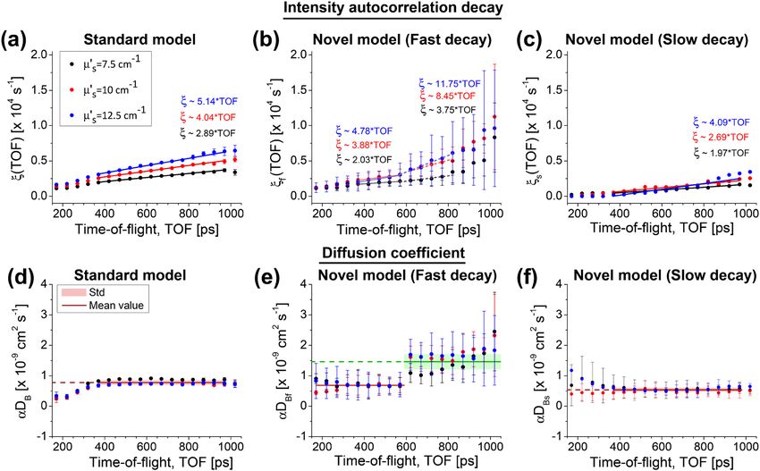
www.nature.com/scientificreports/
Figure 1. Time-domain diffuse correlation spectroscopy in samples composed of particles moving at different
speeds. (a) The light emerging from the source is multiply scattered from slowly (orange), and rapidly (red)
moving particles inside the sample, and then reaches the detector. As the scattering particles move, the photon
light paths change over time (solid and dashed lines), leading to intensity fluctuations at the detector (b). (c)
The larger the particle speed, the more rapid intensity fluctuations. Thus, the intensity autocorrelation function
(ACF) of the rapidly moving particles decays faster (red line) than that of slow particles (orange line). However,
the total ACF (black line) contains contributions from all photons. We disentangle these contributions using a
multi exponential fitting. As the time-of-flight increases (late time gate), we register lower number of correlated
photons. Hence, the intensity autocorrelation contrast decreases.
Potentially, the above issues could be solved by supplementing DCS with a mechanism for probing optical
field fluctuations with a time-of-flight (TOF) resolution. Changes in blood flow in deep tissue (long TOFs) would
then be quantified independently on the changes appearing in superficial regions (short TOFs). The pioneering
contribution in this area comes from Yodh et al., who introduced pulsed diffusing wave spectroscopy (PDWS)11.
In PDWS, the TOF-resolved field fluctuations are sensed with the nonlinear optical mixing through the second-
harmonic generation. Interferometric near-infrared spectroscopy (iNIRS) also quantifies TOF-resolved dynam-
ics in the turbid media12, rodent brain in vivo13, and humans in vivo14 through Fourier-domain interferometric
detection.
Another promising approach is the time-domain (TD-) D CS9,15–18. Sutin et al. introduced this technique and
utilized it to probe cerebral blood flow in rodent brains at short SDS < 1 cm15. Pagliazzi and others implemented
TD-DCS using high coherence l aser16, and measured the relative blood flow index (rBFI) in the human forearm
during the cuff occlusion challenge at SDS = 1 cm16 and quasi-null SDS17. Tamborini et al. demonstrated the port-
able version of the TD-DCS system9, while Colombo et al. developed TD-DCS above the water absorption peak18.
In TD-DCS, the light from a pulsed laser is injected into the sample through the multi-mode fiber (MMF),
and the diffusively reflected light is collected with the single-mode fiber (SMF), and detected with a single-photon
avalanche detector (SPAD) (Fig. 1). Similarly as in the time-domain near-infrared spectroscopy (TD-NIRS)19,20,
the detected photons are time-tagged with time-correlated single-photon counting (TCSPC). However, unlike
TD-NIRS, TD-DCS uses two tags. The first tag corresponds to the time needed for the photon to travel from the
source to the detector, and is used to estimate the photon time-of-flight (TOF). The second tag corresponds to
the absolute arrival time since the measurement was started, and is employed to determine intensity autocorrela-
tion function (intensity ACF). Such a two-dimensional gating allows quantifying BFI with the TOF resolution
through the TOF-resolved intensity ACF, commonly defined a s15:
g2 (ts , τ ) = �I(ts , t)I(ts , t + τ )�t / �I(ts , t)�2t , (1)
where ts denotes the time-of-flight, τ is the autocorrelation lag time, and . . .
t denotes temporal averaging with
respect to t distinct from ts.
In most of the TD-DCS studies the measured time-of-flight-resolved intensity autocorrelation function,
ĝ2 (ts , τ ) is fit to the following model (Siegert relationship)15:
g2(1) (ts , τ ) = 1 + β|g1(1) (ts , τ )|2 , (2)
(1)
where g1 (ts , τ ) = exp [−ξ(ts )τ ] is the single exponential optical field autocorrelation function. The symbol
ξ(ts ) stands for the TOF-dependent ACF decay, whose particular form depends on the underlying model for the
scatterers movement, and β is the intensity ACF c ontrast21.
The above approach presumes that all scatterers move, on average, at the same speed. However, this assump-
tion holds well only for homogeneous samples. On the contrary, biological organs comprise tissues of different
kinds, including epithelial (skin), adipose, and muscle tissues. Due to the difference between the metabolism of
each layer22, cells in those tissues can move at different s peeds7. This effect impacts the DCS and TD-DCS because
the light injected to the organ through the skin is scattered by different particles before reaching the detector
Scientific Reports | (2021) 11:1817 | https://doi.org/10.1038/s41598-021-81448-5 2
Vol:.(1234567890)
www.nature.com/scientificreports/
(Fig. 1a). The detected intensity of such multiply-scattered light contains contributions from all scattering events.
To accurately quantify the blood flow, we need to resolve those contributions. It is thus reasonable to postulate
that the field ACF is a convex sum:
M M
(M)
g1 (ts , τ ) = am exp [−ξm (ts )τ ], am = 1. (3)
m=1 m=1
We now have M exponential terms with distinct, TOF-resolved decays ξm (ts ). Each term corresponds to
optical fields associated with photons scattered from particles moving at different speeds over the experimental
time scale, τ . The summation in Eq. (3) reflects the fact that different scatterers move independently. Hence,
the corresponding scattered fields Um (ts , τ ) are uncorrelated with each other, which formally is expressed as
�Um (ts , t)Un (ts , t + τ )�t = 0 for m = n.
Our approach extends previous studies, in which turbid samples are envisioned as a composition of static and
dynamic particles23,24. Based on this, a phenomenological model, that uses a sum of two negative exponentials (for
slow and fast scatterers) and a constant offset (for static particles) was used to estimate cerebral blood flow with
iNIRS14. Here, by following the concept from the laser Doppler flowmetry to resolve particle speed distribution
in the s ample25, we use the general form of g1(M) (ts , τ ) comprised of M components. We then, substitute Eq. (3)
into Eq. (2) to obtain the novel model for TD-DCS:
(M) (M)
g2 (ts , τ ) = 1 + β|g1 (ts , τ )|2
2
(4)
M
= 1 + β am exp [−ξm (ts )τ ] .
m=1
(M)
Finally, we fit g2 (ts , τ ) to the experimentally estimated ĝ2 (ts , τ ) from the TD-DCS setup sketched in Fig. 1a.
This fitting yields TOF-resolved decays ξm (ts ), from which we obtain either diffusion coefficients, αDB,m in
phantoms or blood flow index in human tissue. In general, we have M decays. We usually interpret the largest
decay as the one related to scatterers located deep into the sample. Photons scattered from the deeply located
scatterers experience many scattering events, and thus decorrelate faster, which is associated with larger ξm (ts ).
Our approach differs from previous theoretical works. Recently, Li et al. introduced an analytical model for
TD-DCS applied to multi-layer heterogeneous turbid s amples26. In their approach g1(M) (ts , τ ) is represented as
a product of several negative exponential functions:
M
M
(M)
g1 (ts , τ ) = exp [−ξm (ts )τ ] = exp − ξm (ts )τ . (5)
m=1 m=1
However, with the above equation we cannot explain experimental observations. In fact, the experimentally
estimated ĝ1 from measured ĝ2 [Eq. (2)] obtained independently by different researchers using various optical sys-
tems can have an offset from static scatterrers13 or exhibit a bi-exponential decay10,14,16,27. Thus, deviating from the
single-exponential decay, predicted by Eq. (5). On the contrary, we validated our approach against measurements
in tissue-mimicking phantoms and humans in vivo, and found that our model fits experimental data very well.
We also note that measured intensity autocorrelation functions, ĝ2 (ts , τ ) depends on the instrument response
function or the IRF28,29. Then, to improve the signal-to-noise ratio, the experimental estimates are integrated over
the photon TOF range, called the time gate. Consequently, the theoretical model can be extended to include both
IRF and the normalized photon distribution of time-of-flight (DTOF) as we demonstrate under methods. Here,
we employ Eq. (4) since we only consider narrow time gates, neglecting the IRF and TOF integration effects.
Results
Tissue‑mimicking phantoms. To validate the feasibility of separating different flows in turbid media,
we performed TD-DCS measurements in liquid phantoms. Each measurement was repeated N = 5 times.
First, we carried out the measurements on three homogeneous phantoms with the same absorption coefficient
(µa = 0.06 cm−1) and the variable reduced scattering (µ′s = 7.5, 10.0, and 12.5 cm−1).
The TOF-resolved intensity ACFs were estimated using a 100 ps width time gate. Then by fitting the stand-
ard model to each ACF curve, we obtain the TOF-resolved autocorrelation decays ξ(ts ) (Fig. 2a), from which
we calculate the diffusion coefficients, αDB (TOF) [see Eq. (9) in Methods]. Figure 2b shows that resulting
values of αDB (TOF) are consistent across phantoms. Lastly, we averaged diffusion coefficients for TOF > 370 ps
( αDB = 1.51 × 10⁻⁹ cm2 s−1), and then use it as the control value for the two-layer liquid phantoms.
The two-layer liquid phantoms were prepared such that the optical properties were kept constant in both
layers, and we reduced the dynamical properties of the top layer. To do so, we mixed the liquid with glycerol
(30% concentration) and controlled optical properties using recipe from Supplementary Fig. S2. The instrument
response function (IRF) and the photon distribution of time-of-flight (DTOF) of the two-layer liquid phantoms
are shown in Supplementary Video S1.
Subsequently, we estimated TOF-resolved intensity ACF using a time gate of 100 ps width. Experimental
estimates were then fit with standard TD-DCS model [Eq. (2)] and novel model [Eq. (4)] with M = 2 exponential
ACFs. The representative fits are depicted in Supplementary Video S1 online. The fitting yielded TOF-resolved
ACF decays, shown in Fig. 3a–c. Now, the novel model provides two ACF decays: fast ξf (ts ) (Fig. 3b) and slow
ξs (ts ) (Fig. 3c). These components are used to determine the corresponding diffusion coefficients for each model
(Fig. 3d–f).
Scientific Reports | (2021) 11:1817 | https://doi.org/10.1038/s41598-021-81448-5 3
Vol.:(0123456789)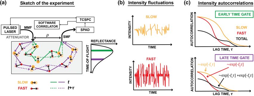
www.nature.com/scientificreports/

                                            Figure 2.  Estimating the diffusion coefficient of homogeneous phantoms with the time-domain diffuse
                                            correlation spectroscopy. (a) The autocorrelation decays were obtained using the standard model for the variable
                                            time-of-flight (TOF). The resulting decays were fitted to a line, from which we estimate the diffusion coefficient
                                            (b).

                                            Figure 3.  Time-domain diffuse correlation spectroscopy measurement in two-layer liquid phantoms with
                                            absorption coefficient (µa = 0.06 cm−1) and variable reduced scattering (µ′s = 7.5, 10.0, and 12.5 cm−1).
                                            (a–c) Estimated TOF-resolved autocorrelation decays and the diffusion coefficients (d–f). The standard model
                                            provides a constant slope of the ACF decays, and thus is incapable to distinguish flows in different layers (d).
                                            On contrary, the fast component of the novel model changes at 600 ps (b), which allows to clearly separate the
                                            depth-dependent diffusion coefficients (e). The slow component of the novel model senses the top layer along
                                            different TOFs by providing a uniform slope of ACF decay (c), and a constant diffusion coefficient (f) close to
                                            the value estimated by the fast component at early TOFs (e).

                                                Figure 3b shows that fast component, ξf (ts ) increases more rapidly for time-of-flights larger than 600 ps.
                                            Consequently, at this transition point, we observe larger values of αDB,f since late photons probe deep phantom
                                            layer with faster particles. Last, the mean diffusion coefficient ( αDB,f = 1.46 × 10⁻⁹ cm2s−1) estimated for the
                                            late time gates (570 − 820 ps) using the fast component [ξf (ts )] of the novel model is almost the same as that of
                                            the homogeneous phantom ( αDB = 1.51 × 10⁻⁹ cm2s−1), indicated in Fig. 2b. Furthermore, the diffusion coef-
                                            ficient obtained from the slow component [ξs (ts )] of the novel model (αDB,s = 5.40 × 10⁻¹⁰ cm2s−1) (Fig. 3f) is
                                            close to the values estimated for the time-of-flight earlier than 600 ps ( αDB,f = 6.88 × 10⁻¹⁰ cm2 s−1) (Fig. 3e).

          Scientific Reports |   (2021) 11:1817 |                https://doi.org/10.1038/s41598-021-81448-5                                                    4

Vol:.(1234567890)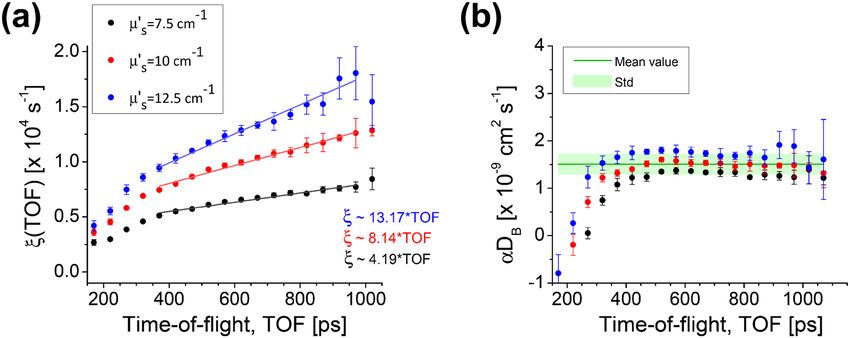
www.nature.com/scientificreports/
Figure 4. In vivo cuff occlusion challenge in human forearm. (a) Experimental sketch. (b) Representative
DTOF, showing the time gates, used for estimating the relative BFI trends (f,g). (c–e) Representative intensity
ACFs of different stages of the measurement. At the baseline, intensity ACF decorrelates much faster (c) than at
the cuff occlusion stage (d). Right after the cuff is released, the intensity ACF is composed of the two ACFs that
decorrelate at different rates (e). The novel model depicts the depth-dependent reactive hyperemia (g), while
conventional TD-DCS model does not (f).
On the contrary, the standard model underestimates diffusion coefficient (αDB = 7.76 × 10⁻¹⁰ cm2 s−1) due to
the influence of the superficial layer.
Human forearm in vivo. Next, we applied TD-DCS to measure blood flow in the cuff occlusion challenge
on the left arm of three healthy volunteers in vivo (Fig. 4a). The representative DTOF is depicted in Fig. 4b. We
estimated intensity ACFs at three different gates, and then fit them using standard and novel models (Fig. 4c–e).
Figure 4c,d shows that the intensity autocorrelation function decorrelates faster at the baseline stage than
during the cuff was occluded. Furthermore, Fig. 4e clearly illustrates the influence of the mixture of slow and
fast blood flows on the ACF just after the cuff deflation. In this case, the ACF decorrelates at different rates, and
the novel model fits very well to, while the standard model deviates from the experimental data.
To quantify blood flow in muscle tissue, we only use the fast decay (because it provides the information
about the rapidly moving scatterers, i.e. blood cells). However, now we interpret the diffusion coefficient as the
blood flow index (BFI). Then, we calculated the relative blood flow index (rBFI) by normalizing the BFIs to the
baseline. To obtain the baseline we averaged datapoints within the 60 s just before the cuff occlusion was applied.
The resulting rBFI trends for the standard and novel models are averaged over all three subjects and depicted
in Fig. 4f,g, respectively. The results obtained for each subject are provided in Supplementary Fig. S1 online. For
the standard model, the rBFI is independent of the time gate. From previous e xperiments7, we expect that rBFI
for late photons, after the cuff is released, provide larger values than that of the early photons (reactive hyperemia
is stronger for deep tissue layers, i.e., muscles). However, when the standard model is used, the rBFI trends do not
exhibit such a behavior. Even though the light paths are distinguished by their TOF, the standard model does not
provide depth selectivity. This means that TOF is insufficient to quantify the blood flow at various tissue layers,
and the use of our approach is warranted.
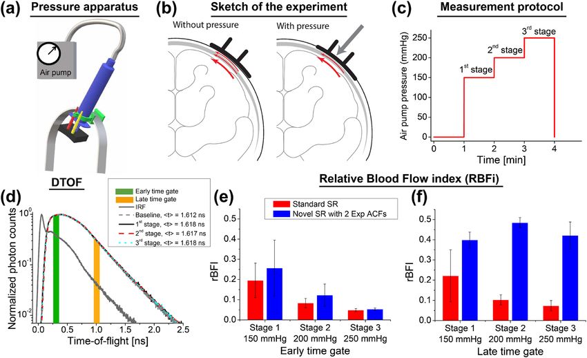
Human forehead in vivo. Finally, we applied TD-DCS in the adult human forehead under controllable
pressure on the forehead skin (Fig. 5). This experiment provides an illustrative example of how the static and
slow scatterers located in extra-cerebral tissue (scalp or skull) contribute to the signal at short source-detector
separation. By pressing the tissue, we change the superficial flow, while cerebral flow remains constant (Fig. 5b).
By analyzing DTOFs we confirmed that optical properties did not significantly change when the pressure
value increased (Fig. 5d). Then, we estimated intensity ACFs, from which we calculated relative BFIs for early and
late time gates (Fig. 5e,f). The BFIs were normalized to the baseline, measured before the pressure was applied.
For the early gate (centered at 0.3 ns), the rBFI decreases with increasing pressure (Fig. 5e). However, we do
not expect a similar behavior for the late time gates (centered at 1 ns). This is because applying pressure on the
scalp blocks blood flow on superficial layers, but the skull prevents this pressure from being applied to the brain
cortex. The rBFI derived from the novel model confirms this hypothesis (Fig. 5f), while the rBFI estimated from
the standard decreases with increasing pressure. Though the novel model works as an additional gating mecha-
nism, supplementing time gating, the two gates might not completely reject photons propagating extracerebral
layers. This issue can also reduce the rBFI compared to the baseline value. Hence even for the novel model, the
Scientific Reports | (2021) 11:1817 | https://doi.org/10.1038/s41598-021-81448-5 5
Vol.:(0123456789)www.nature.com/scientificreports/
Figure 5. Measuring the relative blood flow index in the human forehead under variable pressure in vivo.
(a) The sketch of the pressure apparatus (a), experiment (b), and tissue pressure protocol (c). (d) IRF and
representative DTOFs for various stages of the experiment. Relative blood flow for early (e) and late time gate (f)
are compared between the standard (red bars) and novel (blue bars) models.
estimated rBFI is still below the baseline value. We expect that this problem can be solved by a more general
fitting approach that includes the effect of IRF.
Discussion and conclusions
In summary, we introduced and applied the novel model for time-domain diffuse correlation spectroscopy
(TD-DCS), enabling independent quantification of various blood flows in human tissue. We demonstrated that
sorting detected photons based on their penetration time in tissue by TD-DCS is insufficient to distinguish blood
flows at different layers. To solve this problem, we applied our novel model, and quantified depth-resolved blood
flows in heterogeneous media, particularly in human tissue. We validated our approach via measurements in
tissue-mimicking phantoms, and the cuff occlusion challenge on the human forearm in vivo.
The diffusion coefficient of the homogeneous liquid phantoms were estimated by using the standard model,
and the averaged value ( αDB = 1.51 × 10⁻⁹ cm2 s−1) was considered as a reference. Next, in the two-layer liq-
uid phantom measurements, we utilized the reference media in the deep layer covered with a liquid phantom
comprising slower scatterers and matched optical properties. Then by employing the novel we quantified the
diffusion coefficient of both layers. The fast component of the novel model recovered the reference value from
the deep layer (αDBf = 1.46 × 10⁻⁹ cm2 s−1), while the slow component estimated the diffusion coefficient of the
top layer, mixed with 30 % glycerol, around 36 % lower than the reference value (αDBs = 5.40 × 10⁻¹⁰ cm2 s−1),
as expected30. Importantly, the standard model was incapable to distinguish variable dynamics in both layers and
provided a constant value of αDB = 7.76 × 10⁻¹⁰ cm2 s−1.
We performed forearm cuff occlusion measurements on healthy adults in vivo. We detected the depth-
resolved blood flow changes by using the fast component of the novel model. We showed a higher magnitude of
hyperemic peak after the cuff pressure deflation corresponding to late time gate, which is due to higher hemo-
dynamic changes in muscle than in adipose tissue7. Importantly, this was not possible with the standard model,
which estimated a similar rBFI trend for early and late time gates. In fact, the magnitude of the hyperemia peak
estimated by the standard model is close to the values measured from the novel model for the early time gate,
which can be due to the long-tailed IRF. The relative rBFI changes for slow components and each subject is
available in Supplementary Fig. S1 online.
Finally, we performed measurements on the forehead of an adult human volunteer under the variable pres-
sure. By employing the novel model we reduced the effects of the superficial layer and obtained a constant level
of deep layer blood flow, during various pressure stages. In order to distinguish the contribution of blood flowing
in the skull from the cortex blood flow, further studies on multi-layers phantoms with a more general approach
are required.
The optical setup suffers from the limited laser coherence length and detected photon count rates. We tack-
led these issues by utilizing short source-detector separation (1 cm) and increasing the recording time. On the
one hand, by increasing collection time we reduce the time-resolution. Thus, we cannot detect fast fluctuations
like pulsatile heart beat. On the other hand, by using short source-detector separations, the detected signals
Scientific Reports | (2021) 11:1817 | https://doi.org/10.1038/s41598-021-81448-5 6
Vol:.(1234567890)www.nature.com/scientificreports/
are significantly affected by superficial layers. By employing our novel processing method we minimize the
contamination from those layers.
Virtually, we can use any number of exponentials [M parameter in Eq. (4)]. However, by increasing M we also
increase the overall number of fitting parameters. Accordingly, the fitting becomes more complex and sensitive
to numerical errors.
In summary, we expect our method to be applicable in scenarios that require short source-detector separa-
tions. For example, brain-computer or body-computer interfacing. Our processing can be applied to any method
that is oriented at quantification of particles movement in scattering medium with scattered light correlations,
including DCS, interferometric NIRS, interferometric diffusing wave spectroscopy (iDWS), and fluorescence
correlation spectroscopy (FCS).
Methods
Optical system. In our TD-DCS system, we use an 80 MHz pulsed laser (LDH-P-C-N-760, PicoQuant),
emitting pulses shorter than 90 ps at a wavelength, of 760 nm. Using the commercial spectrometer we esti-
mated the coherence length of this laser to 6.1 mm. Light from the laser is delivered to the sample surface
through a 1 mm core diameter multi-mode fiber with a numerical aperture (NA) of 0.39. A variable neutral
density attenuator was used to set the average optical power delivered to the surface of the medium to 12 mW.
The diffusively reflected light is collected by a single-mode fiber, located at a distance ρ from the source, and
detected with a single-photon avalanche diode (SPAD) detector (PDM, Micro Photon Devices). The SPAD out-
put is time-correlated with a reference signal from the laser controller using the time-correlated single-photon
counting (TCSPC) module (SPC-130, Becker&Hickl). The TCSPC provides the time-of-flight and the absolute
photon arrival time of each detected photon with the temporal resolutions of 3.5 ps (for the photon distribution
of time-of-flight or DTOF) and 12.5 ns (for intensity autocorrelations), respectively.
The instrument response function (IRF), affecting the true DTOF, is measured by facing the source and detec-
tion fibers in front of each other. The tip of the detection fiber is covered with a sheet of white paper to fill up the
full numerical aperture of the fiber31. By doing so, we estimated the IRF full width at half maximum (FWHM)
to 100 ps. All measurements were performed in reflection geometry at source-detector separation, ρ = 1 cm. To
ensure the conditions for all the experiments and minimize the environmental noise, the measurements were
performed in a dark room at a temperature of about 25 ◦ C.
Raw data processing. The output of the optical system (from TCSPC module) can be represented as a two-
dimensional dataset, N(ts , t). That is the number of photons, traveling from source to detector at a particular
TOF with the absolute arrival time, t. We process TCSPC data to achieve the photon distribution of time-of-
flight (DTOF) by integrating photon counts with the same TOFs:
T
DTOF(ts ) = N(ts , t)dt, (6)
0
where T is the total measurement time. Photon counts N(ts , t) are binned together within the time gate Tgw of
fixed width 100 ps, and converted to intensities:
Tgw /2
Î(ts , t) = Ep N(ts + tgw , t)dtgw , (7)
−Tgw /2
where Ep = hc/ is the single-photon energy (h is the Planck constant, and c stands for the speed of light in
vacuum).
Then, we estimate intensity ACF as:
Î(ts , t)Î(ts , t + τ )
t
ĝ2 (ts , τ ) =
2 . (8)
Î(ts , t)
t
For all reported experiments, ĝ2 (ts , τ ) was obtained from a rectangular time gate with 100 ps width, which
offers the best trade-off between the signal-to-noise ratio and the intercept of the normalized intensity autocor-
relation function. Furthermore, the ACFs were estimated from the data recorded during 60 s, except the pressure-
dependent measurements. Due to the employed protocol in the forehead pressure experiment, the integration
time was reduced to 30 s to extract more than one data point without overlapping the neighbor stages at each
part of the measurement.
Estimating diffusion coefficient and blood flow index. To determine diffusion coefficient and
blood flow index we proceed as follows. We fit g2(M) (ts , τ ) with variable M [Eqs. (3), (4)] to the experimen-
tally estimated ĝ2 (ts , τ ) from the TD-DCS setup sketched in Fig. 1a. Using the Brownian motion m odel6, in
which ξm (ts ) ∝ µ′s αDB,m ts (α is the parameter, that traditionally represents the fraction of dynamic to scattering
events6, and µ′s is the reduced scattering), we estimate the diffusion coefficient (αDBm) of the mth component.
In practice, the decay rates for short TOFs deviate from the Brownian motion model predictions. Therefore,
we exclude those TOFs from further analysis, in which we fit the linear model ξm (ts ) = p1 × ts + p0 [ s−1] to the
experimentally estimated TOF-resolved ACF decays. The fitting procedure yields the slope, p1 = 2k2 µ′s cαDB,m /n
Scientific Reports | (2021) 11:1817 | https://doi.org/10.1038/s41598-021-81448-5 7
Vol.:(0123456789)www.nature.com/scientificreports/
(k = 2πn/ , n is the refractive index, c denotes the speed of light in vacuum), and an offset, p0. To obtain an
accurate estimate of the αDB,m we subtract an offset and calculate αDB,m as:
ξm − p0 n
αDB,m (ts ) = . (9)
2k2 µ′s cts
When applying the above approach in tissue we call αDB,m (ts ) as the blood flow index (BFI).
Phantom experiments. The measurements on fluid phantoms were performed in a custom-made cubic
compartment with a side length of 6 cm. This chamber has black walls and simulates the semi-infinite geometry
to satisfy light diffusion assumptions. The front plate of the compartment includes two tiny holes, with diam-
eters of 2.5 mm, covered by a 23 µm thick transparent Mylar film to fix the fibers with 10 mm separation on the
phantom surface.
First, we carried out the measurements on homogeneous liquid phantoms. The liquid tissue-mimicking phan-
toms were made by mixing homogenized milk (3.2 % fat), distilled water, and black ink (Rotring, Germany). The
phantoms had the same absorption coefficient (µa = 0.06 cm−1), but differed in reduced scattering coefficients
(µ′s = 7.5 − 12.5 cm−1 in steps of 2.5 cm−1). During the measurements on homogeneous phantoms, the com-
partment was uniformly filled by the phantoms. While, in order to perform measurements on two-layer liquid
phantoms, a 23 µm thick Mylar sheet was fixed inside the compartment, parallel to the front plate, and with
0.5 cm separation from this plate, to separate the phantom layers. In each measurement, the optical properties
of the liquids used in upper and deeper compartments were matched. The homogeneous phantoms were used
in the deeper compartment, while the liquid in the upper part was mixed with glycerol (30% concentration) to
slow down the scatterers30.
To tune the optical properties between the media, we first quantified the µ′s based on the concentrations of
scattering component (milk) and glycerol [Supplementary Fig. S2]. Then we added black ink (Rotring) to increase
the absorption coefficient of the phantom to µa = 0.06 cm−1 by using the recipe f rom32. The optical properties
of each sample were controlled using a TD-NIRS setup and moment a pproach19,33, separately. This system was
constructed using the same laser diode as in our TD-DCS instrument (operating at a wavelength of 760 nm) and
a photomultiplier detector (PMC-100, Becker & Hickl) coupled with a multi-mode fiber (core diameter 600 µm).
To obtain a similar signal-to-noise ratio across all the phantom measurements, the optical power of the
source was controlled with the neutral density attenuator, located in front of the laser head (Fig. 1a). We tuned
the count rate to 1362 Kcps for each measurement. The raw signals of each experiment were recorded in five
repetitions with 1 min collection time.
In vivo measurement protocols. We applied the TD-DCS method to quantify blood flow index (BFI)
time courses during the cuff occlusion challenge in the human forearm and forehead pressure measurement
on adult healthy volunteers in vivo. These measurements were performed at 1 cm source-detector separations
and the optical power of the source delivered to the tissue surface was 12 mW. All experimental procedures and
protocols were reviewed and approved by the Commission of Bioethics at the Military Institute of Medicine,
Poland (permission no. 90/WIM/2018). The experiments were conducted following the tenets of the Declaration
of Helsinki. Written informed consent was obtained from all subjects before TD-DCS sensing and explaining
all possible risks related to the examination. The physiological parameters of the participants are given in the
Supplementary Table S1 online.
To monitor blood flow changes during the cuff occlusion challenge, the source and detector fibers were fixed
in a black 3D printed square fiber holder, with a side length of 6 cm. The fiber holder was secured over the flexor
carpi radialis with an elastic bandage. The organ went through three different physiological stages. First, the rest
state was measured for 2 min to determine the baseline blood flow index (BFI). Second, the blood pressure cuff
was inflated quickly to 180 mmHg and was held for 2 min. Third, the cuff was released, and we measured the
recovery state for 3 min. This measurement was carried out on three volunteers.
To apply a uniform and controllable pressure on the participant forehead, we developed a pressing mecha-
nism, comprising a cylinder pumped by air at tunable pressure levels, and its connecting rod was attached to the
probe mounting the optodes (Fig. 5a). The probe was a black 3D-printed panel which held source and detector
fibers by 1 cm separation, and covered the tissue curvature. The measurement was carried out on one of the
volunteers and repeated three times in the same day. The participant was asked to lay supine on a bed, and the
probe placed on the subject’s scalp directly over the right prefrontal cortex. One minute rest started the experi-
ment, and then the tissue was pressed in three stages with variable pressure: 150, 200, and 250 mmHg. Each
pressure was applied for 1 min (Fig. 5c).
Statistical analysis of the fitting. To quantify fitting with standard and novel models, we performed a
statistical analysis of the sample fits we achieved for in vivo experiments (cuff occlusion challenge on participant
C). We used the intensity autocorrelations estimated at the middle time gate (centered at the 0.57 ns). Then,
we performed fitting for the standard and novel model and calculated the following statistical tests: the sum of
squares (SSE), R-square, adjusted R-square, degree of freedom in error (DFE), and the root mean squared error
of standard error (RMSE). The results are summarized in Table 1.
General expression for the intensity autocorrelation function. The measured TOF-resolved inten-
sity autocorrelation function ĝ2 (ts , τ ) depends on the instrument response function or the IRF, and the photon
Scientific Reports | (2021) 11:1817 | https://doi.org/10.1038/s41598-021-81448-5 8
Vol:.(1234567890)www.nature.com/scientificreports/
Model Number of parameters R2 Adjusted R2 DFE SSE RMSE
Novel 4 0.95 0.94 56 7.81E−3 1.18E−2
Standard 2 0.80 0.80 58 3.00E−2 2.28E−2
Table 1. Statistical analysis of the fitting with standard and novel model.
time-of-flight distribution, when experimental estimates are integrated over the TOF. Thus, under the validity of
Eq. (2), we can include those effects as follows28:
M
2
Tgw /2
(M)
(10)
′ ′ ′ ′
g2 (ts , τ , Tgw ) = 1 + β dt P (ts + ts ) am exp −ξm (ts + ts )τ ,
−Tgw /2 s
m=1
where Tgw is the gate width, and P ′ (ts ) is the normalized measured photon distribution of time-of-flight (DTOF),
which is related to the true photon TOF distribution P(ts ) via a convolution ( ⋆ ) with the IRF, I0 (ts ):
1
P ′ (ts ) = P(ts ) ⋆ I0 (ts ), (11)
NP
∞
where NP = −∞ dts P(ts ) ⋆ I0 (ts ) is the normalization factor.
Received: 14 September 2020; Accepted: 28 December 2020
References
1. Hoskins, P. Measurement of arterial blood flow by doppler ultrasound. Clin. Phys. Physiol. Meas. 11, 1 (1990).
2. Liebert, A., Leahy, M. & Maniewski, R. Multichannel laser-doppler probe for blood perfusion measurements with depth discrimi-
nation. Med. Biol. Eng. Comput. 36, 740–747 (1998).
3. Izatt, J. A., Kulkarni, M. D., Yazdanfar, S., Barton, J. K. & Welch, A. J. In vivo bidirectional color doppler flow imaging of picoliter
blood volumes using optical coherence tomography. Opt. Lett. 22, 1439–1441 (1997).
4. Durduran, T. et al. Spatiotemporal quantification of cerebral blood flow during functional activation in rat somatosensory cortex
using laser-speckle flowmetry. J. Cereb. Blood Flow Metab. 24, 518–525 (2004).
5. Pavlidis, I. et al. Interacting with human physiology. Comput. Vis. Image Underst. 108, 150–170 (2007).
6. Durduran, T. & Yodh, A. G. Diffuse correlation spectroscopy for non-invasive, micro-vascular cerebral blood flow measurement.
Neuroimage 85, 51–63. https://doi.org/10.1016/j.neuroimage.2013.06.017 (2014).
7. Yu, G. et al. Time-dependent blood flow and oxygenation in human skeletal muscles measured with noninvasive near-infrared
diffuse optical spectroscopies. J. Biomed. Opt. 10, 024027. https://doi.org/10.1117/1.1884603 (2005).
8. Patterson, M. S., Chance, B. & Wilson, B. C. Time resolved reflectance and transmittance for the non-invasive measurement of
tissue optical properties. Appl. Opt. 28, 2331–6. https://doi.org/10.1364/AO.28.002331 (1989).
9. Tamborini, D. et al. Portable system for time-domain diffuse correlation spectroscopy. IEEE Trans. Biomed. Eng. 66, 3014–3025.
https://doi.org/10.1109/TBME.2019.2899762 (2019).
10. Sathialingam, E. et al. Small separation diffuse correlation spectroscopy for measurement of cerebral blood flow in rodents. Biomed.
Opt. Express 9, 5719–5734. https://doi.org/10.1364/BOE.9.005719 (2018).
11. Yodh, A. G., Kaplan, P. D. & Pine, D. J. Pulsed diffusing-wave spectroscopy: high resolution through nonlinear optical gating. Phys.
Rev. B Condens. Matter 42, 4744–4747 (1990).
12. Borycki, D., Kholiqov, O., Chong, S. P. & Srinivasan, V. J. Interferometric near-infrared spectroscopy (INIRS) for determination
of optical and dynamical properties of turbid media. Opt. Express 24, 329–54. https://doi.org/10.1364/OE.24.000329 (2016).
13. Borycki, D., Kholiqov, O. & Srinivasan, V. J. Reflectance-mode interferometric near-infrared spectroscopy quantifies brain absorp-
tion, scattering, and blood flow index in vivo. Opt. Lett. 42, 591–594. https://doi.org/10.1364/OL.42.000591 (2017).
14. Kholiqov, O., Zhou, W., Zhang, T., Du Le, V. . N. . & Srinivasan, V. . J. . Time-of-flight resolved light field fluctuations reveal deep
human tissue physiology. Nat. Commun. 11, 391. https://doi.org/10.1038/s41467-019-14228-5 (2020).
15. Sutin, J. et al. Time-domain diffuse correlation spectroscopy. Optica 3, 1006–1013. https: //doi.org/10.1364/Optica .3.001006 (2016).
16. Pagliazzi, M. et al. Time domain diffuse correlation spectroscopy with a high coherence pulsed source: in vivo and phantom results.
Biomed. Opt. Express 8, 5311–5325. https://doi.org/10.1364/Boe.8.005311 (2017).
17. Pagliazzi, M. et al. In vivo time-gated diffuse correlation spectroscopy at quasi-null source-detector separation. Opt. Lett. 43,
2450–2453. https://doi.org/10.1016/j.neuroimage.2013.06.0171 (2018).
18. Colombo, L. et al. In vivo time-domain diffuse correlation spectroscopy above the water absorption peak. Opt. Lett. 45, 3377–3380.
https://doi.org/10.1016/j.neuroimage.2013.06.0172 (2020).
19. Liebert, A. et al. Time-resolved multidistance near-infrared spectroscopy of the adult head: intracerebral and extracerebral absorp-
tion changes from moments of distribution of times of flight of photons. Appl. Opt. 43, 3037–3047. https: //doi.org/10.1016/j.neuro
image.2013.06.0173 (2004).
20. Torricelli, A. et al. Time domain functional NIRS imaging for human brain mapping. Neuroimage 85(Pt 1), 28–50. https://doi.
org/10.1016/j.neuroimage.2013.05.106 (2014).
21. Lemieux, P. A. & Durian, D. J. Investigating non-Gaussian scattering processes by using nth-order intensity correlation functions.
J. Opt. Soc. Am. Opt. Image Sci. Vis. 16, 1651–1664. https://doi.org/10.1364/Josaa.16.001651 (1999).
22. Binzoni, T. et al. Energy metabolism and interstitial fluid displacement in human gastrocnemius during short ischemic cycles. J.
Appl. Physiol. 85, 1244–1251 (1998).
23. Boas, D. A. & Yodh, A. G. Spatially varying dynamical properties of turbid media probed with diffusing temporal light correlation.
J. Opt. Soc. Am. Opt. Image Sci. Vis. 14, 192–215. https://doi.org/10.1364/Josaa.14.000192 (1997).
24. Borycki, D., Kholiqov, O. & Srinivasan, V. J. Interferometric near-infrared spectroscopy directly quantifies optical field dynamics
in turbid media. Optica 3, 1471–1476. https://doi.org/10.1016/j.neuroimage.2013.06.0177 (2016).
Scientific Reports | (2021) 11:1817 | https://doi.org/10.1038/s41598-021-81448-5 9
Vol.:(0123456789)www.nature.com/scientificreports/
25. Liebert, A., Zolek, N. & Maniewski, R. Decomposition of a laser-doppler spectrum for estimation of speed distribution of particles
moving in an optically turbid medium: Monte carlo validation study. Phys. Med. Biol. 51, 5737–51. https://doi.org/10.1016/j.neuro
image.2013.06.0178 (2006).
26. Li, J., Qiu, L., Poon, C.-S. & Sunar, U. Analytical models for time-domain diffuse correlation spectroscopy for multi-layer and
heterogeneous turbid media. Biomed. Opt. Express 8, 5518–5532. https://doi.org/10.1016/j.neuroimage.2013.06.0179 (2017).
27. Sathialingam, E. et al. Hematocrit significantly confounds diffuse correlation spectroscopy measurements of blood flow. Biomed.
Opt. Express 11, 4786–4799. https://doi.org/10.1117/1.18846030 (2020).
28. Cheng, X. J. et al. Time domain diffuse correlation spectroscopy: modeling the effects of laser coherence length and instrument
response function. Opt. Lett. 43, 2756–2759. https://doi.org/10.1117/1.18846031 (2018).
29. Colombo, L. et al. Effects of the instrument response function and the gate width in time-domain diffuse correlation spectroscopy:
model and validations. Neurophotonics 6, 1–9. https://doi.org/10.1117/1.18846032 (2019).
30. Cortese, L. et al. Liquid phantoms for near-infrared and diffuse correlation spectroscopies with tunable optical and dynamic
properties. Biomed. Opt. Express 9, 2068–2080 (2018).
31. Liebert, A., Wabnitz, H., Grosenick, D. & Macdonald, R. Fiber dispersion in time domain measurements compromising the accu-
racy of determination of optical properties of strongly scattering media. J. Biomed. Opt. 8, 512–516. https: //doi.org/10.1117/1.15780
88 (2003).
32. Choe, R. Diffuse optical tomography and spectroscopy of breast cancer and fetal brain. Ph.D. dissertation (2005).
33. Liebert, A. et al. Evaluation of optical properties of highly scattering media by moments of distributions of times of flight of photons.
Appl. Opt. 42, 5785–5792. https://doi.org/10.1117/1.18846034 (2003).
Acknowledgements
We acknowledge support from the following grants: Horizon 2020: Marie Sklodowska-Curie Innovative Training
Networks (675332, Bitmap); Horizon 2020: research and innovation program (666295, CREATE); Narodowe
Centrum Nauki (NCN) (Maestro 2016/22/A/ST2/00313, Preludium 2019/33/N/ST7/03024).
Author contributions
S.S. assembled the setup with the support of P.S and M.K. S.S. conceived the experiments and processed raw data.
Ż.P. provided biomedical ethical approval. D.B. and S.S. designed experiments. D.B. analyzed data and wrote
the manuscript with the input from all authors. A.L. provided funding, project’s idea, and general support. All
authors reviewed the manuscript.
Competing interests
The authors declare no competing interests.
Additional information
Supplementary Information The online version contains supplementary material available at https://doi.
org/10.1038/s41598-021-81448-5.
Correspondence and requests for materials should be addressed to D.B.
Reprints and permissions information is available at www.nature.com/reprints.
Publisher’s note Springer Nature remains neutral with regard to jurisdictional claims in published maps and
institutional affiliations.
Open Access This article is licensed under a Creative Commons Attribution 4.0 International
License, which permits use, sharing, adaptation, distribution and reproduction in any medium or
format, as long as you give appropriate credit to the original author(s) and the source, provide a link to the
Creative Commons licence, and indicate if changes were made. The images or other third party material in this
article are included in the article’s Creative Commons licence, unless indicated otherwise in a credit line to the
material. If material is not included in the article’s Creative Commons licence and your intended use is not
permitted by statutory regulation or exceeds the permitted use, you will need to obtain permission directly from
the copyright holder. To view a copy of this licence, visit http://creativecommons.org/licenses/by/4.0/.
© The Author(s) 2021
Scientific Reports | (2021) 11:1817 | https://doi.org/10.1038/s41598-021-81448-5 10
Vol:.(1234567890)You can also read