Formal Constraint-based Compilation for Noisy Intermediate-Scale Quantum Systems
←
→
Page content transcription
If your browser does not render page correctly, please read the page content below
Formal Constraint-based Compilation
                                                       for Noisy Intermediate-Scale Quantum Systems
                                              Prakash Muralia,∗, Ali Javadi-Abharib , Frederic T. Chongc , Margaret Martonosia
                                                                                   a
                                                                                    Princeton University
                                                                       b
                                                                           IBM Thomas J. Watson Research Center
                                                                                  c
                                                                                    University of Chicago
arXiv:1903.03276v1 [cs.PL] 8 Mar 2019

                                        Abstract
                                        Noisy, intermediate-scale quantum (NISQ) systems are expected to have a few hundred
                                        qubits, minimal or no error correction, limited connectivity and limits on the number of
                                        gates that can be performed within the short coherence window of the machine. The past
                                        decade’s research on quantum programming languages and compilers is directed towards
                                        large systems with thousands of qubits. For near term quantum systems, it is crucial to
                                        design tool flows which make efficient use of the hardware resources without sacrificing the
                                        ease and portability of a high-level programming environment. In this paper, we present
                                        a compiler for the Scaffold quantum programming language in which aggressive optimiza-
                                        tion specifically targets NISQ machines with hundreds of qubits. Our compiler extracts
                                        gates from a Scaffold program, and formulates a constrained optimization problem which
                                        considers both program characteristics and machine constraints. Using the Z3 SMT solver,
                                        the compiler maps program qubits to hardware qubits, schedules gates, and inserts CNOT
                                        routing operations while optimizing the overall execution time. The output of the optimiza-
                                        tion is used to produce target code in the OpenQASM language, which can be executed on
                                        existing quantum hardware such as the 16-qubit IBM machine. Using real and synthetic
                                        benchmarks, we show that it is feasible to synthesize near-optimal compiled code for current
                                        and small NISQ systems. For large programs and machine sizes, the SMT optimization
                                        approach can be used to synthesize compiled code that is guaranteed to finish within the
                                        coherence window of the machine.
                                        Keywords: Quantum compilation, SMT optimization, Quantum computing

                                        1. Introduction
                                           The promise of quantum computing (QC) is to provide the hardware and software envi-
                                        ronment for tackling classically-intractable problems. The fundamental building block of a
                                          ∗
                                            Corresponding author. Full address: Department of Computer Science, Princeton University, 35, Olden
                                        Street, Princeton NJ 08540
                                            Email addresses: pmurali@princeton.edu (Prakash Murali), ali.javadi.abhari@gmail.com (Ali
                                        Javadi-Abhari), chong@cs.uchicago.edu (Frederic T. Chong), mrm@princeton.edu (Margaret
                                        Martonosi)
                                        Accepted for publication in Microprocessors and Microsystems                           March 11, 2019
quantum computer is a qubit or quantum bit. In the circuit model of quantum computation,
quantum programs can be viewed as a series of operations (gates) applied on a set of qubits.
These gates may act on a single qubit or on states constructed using multiple qubits.
Building operational quantum computers requires overcoming significant implementation
challenges. For useful quantum computation, the state of a qubit should be coherent for
a long duration of time, the error rates of gates should be low and unwanted quantum
interactions should be minimized.
QC’s hardware challenges have been partially overcome on small scales (5-20 qubits)
using Nuclear Magnetic Resonance [1, 2], trapped ions [3, 4], and superconducting qubits
[5, 6] among others. Current systems using these technologies have limited coherence time
(few hundred microseconds for superconducting qubits), noisy operations (error rates close
to 0.01), and limited qubit connectivity. As implementation techniques improve, these Noisy
Intermediate Scale Quantum (NISQ) systems are expected to scale to a few hundred qubits,
still with minimal or no error correction and limited connectivity. NISQ systems will also
have limited coherence time, allowing at most a few thousand gates to be executed [7].
The last decade’s research on quantum computing and compilers has focused on methods
for reliable fault tolerant computation using large machines with thousands of qubits [8, 9,
10]. Under tight NISQ constraints, however, it is crucial to design tool flows which make
efficient use of the limited hardware resources without sacrificing the ease and portability
of a high-level programming environment. In this vein, this paper describes and evaluates
a compiler for programs written in a high-level language targeted for NISQ machines with
hundreds of qubits.
Our compiler takes as input a QC program written in the Scaffold language. The Scaf-
fold language is a QC extension of C. Scaffold features automated gate decomposition and
quantum logic synthesis from classical operations. Scaffold programs are independent of the
size, qubit technology, connectivity, and error characteristics of the machine. These features
provide portability and allow users to express their algorithms at a high level—in terms
of logic operations and quantum functions, rather than a more circuit-oriented gate-level
description of the intended computation.
To compile Scaffold programs for NISQ systems, we use an optimization based approach.
We express the compilation problem as a constrained optimization problem which incorpo-
rates both program and machine characteristics. Using the Z3 Satisfiability Modulo Theory
(SMT) solver [11], the compiler maps program qubits to hardware qubits, schedules gates,
and inserts CNOT routing operations while optimizing the overall execution time. The out-
put of the solver is a near-optimal spatiotemporal mapping that is used to produce target
code in the OpenQASM language. The target code can be directly executed on existing
quantum hardware such as the 16-qubit machine from IBM. To scale our method to large
qubit and gate count, we have developed a heuristic approach which also uses the SMT
solver.
Our experiments demonstrate the optimal compilation of programs for the Bernstein-
Vazirani algorithm and execution results from real hardware. Using a collection of real and
synthetic benchmarks, we show that near-optimal compilation is feasible for systems with
small qubit count and limited coherence time. Our results also show that the heuristic
2method scales to large qubit and gate count, and can efficiently fit programs to execute
within the coherence window of the machine.
The main contributions of this paper are as follows:
• We develop an end-to-end framework based on constrained optimization to compile
high level quantum programs for near term NISQ systems.
• Using real and synthetic benchmarks, we demonstrate that the constraint-based com-
piler can be used for near-optimal compilation on current and near term systems.
• We propose a heuristic method for compiling programs for machines with large qubit
and gate counts. The heuristic method uses optimization to fit the execution schedule
of a program within the coherence window of the machine.
• We demonstrate that our heuristic method scales to large programs. For large pro-
grams on 128 and 256 qubits, we exhibit cases where the SMT solver can fit all the
gates within the allowed coherence window, while a greedy scheduling method cannot.
The rest of the paper is organized as follows: Section 2 discusses related work and Section
3 provides an overview of NISQ systems and the Scaffold language. Section 4 presents the
key ideas for NISQ compilation. Sections 5-7 develop the near-optimal compilation method
using the SMT solver. In Section 8, we describe a fast heuristic method. Sections 9-12
present experimental setup and results.
2. Related Work
Many quantum programming languages and compilers have been developed with the
goal of simplifying and abstracting quantum programming from the low level details of the
hardware. These includes works such as Quipper [12, 13], which is a domain specific language
embedded in Haskell, and LIQUi|i [14] which uses the F# language. These languages offer
functionality for quantum circuit description, classical control and compilation and circuit
generation. ProjectQ [15, 16], based on Python, is a framework which allows simple quantum
circuit description and compilation for different backends. OpenQASM [17] is a low level
language to specify a quantum execution at a gate level. It is used as an interface for near
term quantum machines [18]. In this paper, we use the Scaffold language which allows
us to describe the quantum circuit at a high level and leverage the rich LLVM compiler
infrastructure for automated program analysis and optimization [19, 20].
In contrast to compilers and frameworks for prior languages, we describe a compilation
approach which considers the machine coherence time as a primary constraint. This formally
guarantees that the compiled code can finish execution before the hardware qubits decohere.
For programs on small NISQ systems, we can also find near optimal compilations, which can
help in mitigating errors due to state decay. Our work provides a toolflow which compiles
high-level Scaffold programs down to a device-independent intermediate representation using
ScaffCC and then efficiently maps and optimizes the intermediate representation for a target
device.
3Quantum circuit compilation has been studied for different hardware technologies and
topologies. Bhattacharjee et al. [21] use an integer linear programming solver to compile
small quantum programs for nearest neighbor architectures. However, their approach is
applicable only for tiny programs with less than 7 qubits and 90 gates. Using the SMT
solver based approach, we demonstrate that near optimal compiled code can be synthesized
for significantly larger configurations. Guerreschi et al. [22] develop a heuristic to schedule
quantum circuits on a linear topology and assume that all gates (including swaps) require
unit time. Venturelli et al. [23] use temporal AI planners for scheduling a certain class of
quantum circuits. Heckey et al. [24] develop heuristic compilation techniques for a SIMD
gate execution model and assume quantum teleportation based communication. [25, 26, 27,
28] are other works on compiling quantum circuits. In contrast to these approaches, we
provide a general end-to-end compilation framework for transforming Scaffold programs to
execution ready OpenQASM code.
Recently, Fu et al. [29], developed QuMA, a microarchitecture for QC systems based
on superconducting qubits. QuMA takes compiler generated quantum instructions as input
and uses micro-instructions to achieve precise timing control of the physical qubits.
3. Preliminaries
3.1. NISQ Systems
NISQ systems encompass near-term quantum computers that are expected to scale up
to a few hundred qubits. They are expected to support a universal gate set, which allows
any computation to be expressed in terms of a small number of basis operations or gates.
Qubits in these systems have to be isolated from each other, and from the environment,
to prevent noise and errors due to unwanted interactions. On the other hand, to perform
two qubit (CNOT) gates, certain pairs of qubits should be able to interact strongly without
influencing neighboring qubits. Hence, NISQ systems are expected to support limited qubit
connectivity where only neighboring qubits can participate in CNOT gates.
Qubits in these systems are expected to have a coherence time of hundreds of microsec-
onds to few milliseconds. The expected gate error rates are in the range 0.001-0.01. These
factors imply that only a few thousand operations can be performed before the quantum
state decoheres. NISQ systems of this scale can potentially have important applications
in quantum chemistry, quantum semidefinite programming, combinatorial optimization and
machine learning [7].
This paper focuses on NISQ systems where the qubits are arranged in the form of a grid.
We assume nearest neighbor connectivity, where two qubits can participate in a CNOT gate
if they are adjacent on the grid. If a CNOT gate is to be performed between two qubits
which are not adjacent, the qubits have to be moved to adjacent locations using a series of
swap operations.
3.2. Scaffold: Quantum Programming Language
Scaffold is a programming language for expressing quantum algorithms. It is an extension
of C with quantum types. The user can specify quantum algorithms using a gate set and
4Figure 1: Overview of the compilation process. The compiler extracts gates from the Scaffold program and
uses it in conjunction with the machine configuration to solve an SMT optimization problem.
use familiar C style functions and loops to modularize the code. A useful feature of Scaffold
is the ability to specify certain quantum algorithms in classical logic, using rkqc modules.
These modules allows users to express quantum computation using well known classical logic
operations. A variety of applications have been expressed in Scaffold, we refer the reader to
[10, 30] for more details.
3.3. ScaffCC Compiler
The ScaffCC compiler for Scaffold uses the LLVM compiler infrastructure to compile
quantum programs, perform resource estimation and apply error correction. ScaffCC uses
the LLVM intermediate representation to transform the program using a set of compilation
passes. These passes include transformations such as loop unrolling, procedure cloning,
automatic Toffoli and rotation decomposition, and conversion of rkqc modules into their
quantum equivalents using RevKit [31]. Since quantum programs are usually compiled
for fixed inputs, ScaffCC includes techniques to resolve classical control dependencies and
produce an intermediate output consisting of only quantum gates. In this paper, we use
the ScaffCC compiler as a frontend to extract a gate-level description of the computation,
which is then used to synthesize code for NISQ machines.
4. Optimization Techniques for NISQ Compilation
Figure 1 shows our overall compilation approach, accepting a Scaffold program as input
and producing OpenQASM target code. To accomplish this, we first extract gates from the
Scaffold program using ScaffCC. The gates extracted from ScaffCC are in terms of program
qubits and are independent of the target device. We develop compilation techniques which
map this gate representation onto a target device using SMT optimization. In the SMT
optimization step, we solve a constrained optimization problem to determine a program
mapping, execution schedule and routing decisions which provide an executable with with
the minimum makespan (execution time). The makespan is the difference between the finish
time of the last gate and the start time of the first gate. Finally, we postprocess the output
of the solver, insert routing operations as computed by the SMT optimization and emit
OpenQASM code.
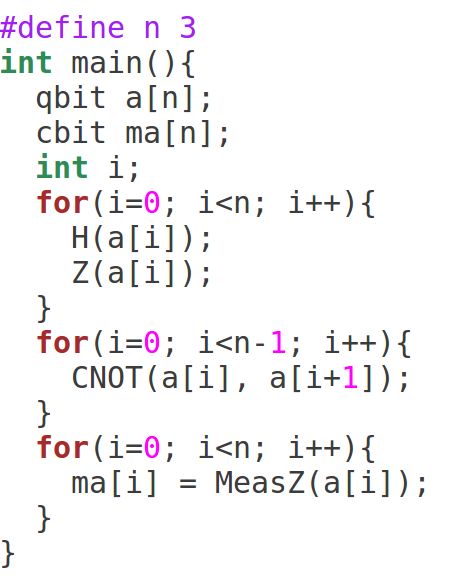
5(a) Scaffold program (b) Gate Dependency Graph
Figure 2: A Scaffold program and the corresponding dependency graph extracted by ScaffCC.
4.1. Gate Extraction
The first module inputs a Scaffold program, and uses the ScaffCC compiler [19] to ex-
tract the LLVM intermediate representation (IR) of the program. Since NISQ systems are
expected to have low coherence time, realistic programs for these systems will only have a
small number of gates (hundreds to thousands). This allows us to consider the whole pro-
gram as a single block for the purpose of optimization. Hence, we unroll all loops and inline
all functions in the program to create a single program module. In addition, ScaffCC also
performs the rotation and gate decomposition, and classical to quantum module conversion
steps, to create a flattened IR for the program.
We use the flattened IR to extract gate level information. The gate level information
specifies each gate in the program, the qubits it acts on, and its input and output dependen-
cies. The output of this module is summarized as a dependency graph for the program. The
vertices of the graph are the gates extracted from the program, and the edges denote the
data dependencies between the gates. Each vertex is annotated with the qubits that a gate
operates on. For example, Figure 2 shows a Scaffold program and its dependency graph.
4.2. Constraint Generation and Optimization
The compiler creates an SMT optimization problem which consists of a set of variables
to track qubit mappings, and gate start times and durations. The optimization constraints
cater to three main factors:
1. Qubit Mapping: The compiler maps program qubits to hardware qubits. The map-
ping constraint specifies that no two program qubits can be mapped to the same
hardware qubit.
2. Gate Scheduling: For each gate extracted from the Scaffold program, the compiler
determines a start time and a duration. For single qubit gates, the duration is the
6execution time of the operation on the target hardware. For CNOT gates, the control
and target qubits may have to be moved using SWAP operations to place the qubits
into adjacent locations on the hardware. The execution time for CNOTs includes the
duration of the SWAP sequence. Gate scheduling addresses data dependencies through
constraints that a gate should start execution only after the gates it depends on finish.
3. CNOT Routing: To prevent routing conflicts, the compiler uses two routing policies
to reason about the SWAP paths of CNOTs. In the first policy, the compiler blocks
the rectangle bounded by the control and target qubit, and routes the SWAPs using
hardware qubits in the rectangle. In the second policy, the compiler selects one of the
two paths along the edge of the bounding rectangle (paths which bend only once) and
performs SWAPs along the selected path. In either case, the SMT constraint is that
if two CNOT gates overlap in time, their SWAP paths through the hardware qubits
should not overlap.
The SMT optimization simultaneously accounts for all three categories of constraints:
qubit mapping decisions affect and are influenced by the gate scheduling and routing de-
cisions. We describe the mapping and scheduling constraints in Section 5 and the routing
constraints in Section 6.
5. SMT Optimization: Qubit Mapping and Gate Scheduling
In this section, we first describe the setup for the optimization problem, followed by the
qubit mapping and gate scheduling constraints.
We process the dependency graph of the program, along with the configuration of the
target machine to create a constrained optimization problem. The program is represented
as a dependency graph P = (V, E) on Q qubits, where V is the set of gates and E is the
set of dependencies. The total number of gates is G = |V |. Each dependency in E is a pair
of gates (i, j) such that gate j can start only after gate i finishes. We assume that for any
qubit, the dependency graph specifies a total ordering of the gates which act on the qubit.
Since ScaffCC decomposes multi-qubit gates, each gate in the dependency graph is either a
single or two qubit gate.
The machine is represented as an MxN grid of hardware qubits. Each qubit is referred
to using its location on the 2-D grid. Qubit (i, j) has hardware CNOT connections to qubits
(i + 1, j) and (i, j + 1). This representation closely models the nearest neighbhor connections
in real systems such as the IBM 16-qubit system [18] and the system in development at
Google [32, 33]. In this paper, we apply swap operations for communication in a restoring
manner i.e., if we apply a set of swaps to change the qubit ordering before a CNOT, we
apply the same swaps after the CNOT to restore the qubit order.
75.1. Qubit Mapping
A program qubit i is mapped to a hardware qubit (qx [i], qy [i]). We add the following
constraints to ensure that mappings respect the distinctness constraint:
qx [i] ∈ [1, M], ∀i ∈ [1, Q] (1)
qy [i] ∈ [1, N], ∀i ∈ [1, Q] (2)
qx [i] 6= qx [j] ∨ qy [i] 6= qy [j], ∀i, j ∈ [1, Q]s.t.i < j (3)
5.2. Gate Scheduling
For every gate j, the solver should determine a start time t[j] and duration d[j]. The
finish time of a gate is t[j] + d[j]. First, we constrain the start and finish times to lie within
the machine’s coherence threshold (T ):
t[j] ∈ [1, T ], ∀j ∈ [1, G] (4)
t[j] + d[j] ≤ T, ∀j ∈ [1, G] (5)
For any single qubit gate j, we can set the duration variable using the duration of the
corresponding hardware gate i.e., d[j] == τ (type(j)). Here, τ is a mapping which specifies
the duration for each gate type. For example, for any Hadamard gate j, we can set the
duration as 1 time slot by hard wiring d[j] == 1.
For CNOT gates, the optimizer has to account for the duration of the hardware CNOT,
and the time required to move the qubits in place before and after the hardware CNOT.
If the L1 distance between the control and target qubit is l, the time taken for the CNOT
is the sum of the durations of l − 1 SWAP gates, the hardware CNOT, and the restoring
sequence of l − 1 SWAP gates. We express this duration as:
define|x| = If-Then-Else(x ≥ 0, x, −x) (6)
dist(c, t) = |qx [c] − qx [t]| + |qy [c] − qy [t]| (7)
d[j] = 2(dist(ctrl(j), targ(j)) − 1) ∗ τ (SW AP ) + τ (CNOT ) (8)
We add constraint 8 for every gate j which is of type CNOT. We note that the time required
for a SWAP can be halved by implementing a meet in the middle policy where both control
and target qubits move in parallel. However, it increases the number of parallel operations
among nearby qubits and can potentially cause more crosstalk errors. In this paper, we
assume that only the control qubit moves to the target qubit using a series of swaps.
Finally, we can represent gate dependencies, by enforcing that a gate j can start only
after its dependent gate i has finished:
t[j] ≥ t[i] + d[i], ∀(i, j) ∈ E (9)
86. SMT Optimization: CNOT Routing
CNOTs which occur between program qubits which are at non-adjacent locations require
communication using SWAP gates. In this section, we describe two communication routing
policies and a pruning strategy to reduce the number of routing constraints.
We observe that the swap paths taken by concurrent CNOTs should not intersect. In
Figure 3a, we illustrate the necessity of having spatially non-overlapping swap paths. If
the control qubits corresponding to the red and blue CNOT pairs are moving towards their
respective targets, it is possible that the control qubits can swap with each other and get
deviated from their routing path. In such cases, the length of the path from the control to
the target is no longer the L1 distance, and it is difficult to quantify the CNOT duration
exactly in constraints 8 and 9. If we consider the case where swap paths overlap spatially,
but qubits use distinct hardware edges at any given time, then the overall qubit mapping
can depend on the relative order in which the swap sequences are executed (not illustrated).
(a) Intersecting swap paths (b) Rectangle Reservation (c) One bend paths
Figure 3: CNOT Routing. Figure 3a illustrates the need for non-overlapping swap paths. Figures 3b and
3c illustrate the two routing policies used in our compiler.
These scenarios motivate us to spatially restrict the swap paths of CNOTs which overlap
in time. We use two routing policies: rectangle reservation and 1-bend paths. These policies
are inspired from similar policies in VLSI routing [34]. We first explain the two routing
policies and then discuss a pruning strategy which reduces the number of routing constraints
required for compilation.
6.1. Rectangle reservation
In rectangle reservation, we reserve the 2-D region bounded by the control and target
qubit locations for the duration of the CNOT. For example, in Figure 3b, the highlighted
rectangle is reserved for the duration of the CNOT. For this policy, we define solver variables
and constraints to check if two CNOT rectangles overlap. The SMT constraint is that if two
CNOTs overlap in time, their bounding rectangles should not overlap in space. The solver
reserves the rectangle for the duration of the CNOT, and the exact swap path within the
rectangle is computed during post-processing.
To implement rectangle reservation, we add variables which track the top-left and bottom-
right locations of each CNOT in the program. Consider a CNOT gate i. We can define
the top-left corner using variables (lx [i], ly [i]) and the bottom-right corner using variables
(rx [i], ry [i]). These variables can be defined using min and max relationships on the control
9and target qubit locations. Denote the control-target rectangle of a CNOT i as Ri . Using
these variables the following constraint detects whether the rectangles of two CNOTs i and
j overlap in space and time:
OverlapInSpace(Ri , Rj ) = ¬(lx [i] > rx [j] ∨ rx [i] < lx [j] ∨ ly [i] > ry [j] ∨ ry [i] < ly [j]) (10)
OverlapInT ime(i, j) = ¬(t[i] > t[j] + d[j] ∨ t[j] > t[i] + d[i]) (11)
The routing constraint for any pair of CNOTs i and j is
OverlapInT ime(i, j) =⇒ ¬OverlapInSpace(i, j) (12)
6.2. 1-Bend Paths
For the second routing policy, we restrict CNOTs to routing paths which bend at most
once on the 2-D grid. There are two such paths along the edges of the bounding rectangle
of the control and target qubit. This policy is very similar to dimension ordered routing.
For example, in Figure 3c, the swaps can be routed using the highlighted red path along
the top edge of the bounding rectangle. In this case, we require the solver to pick one of
the two paths using a variable which determines the bend point or routing junction. 1-bend
paths are advantageous because they block less resources than rectangle reservation at run
time. However, the solver requires additional compile time to determine the exact path
during optimization.
For 1-bend paths, we can write constraints similar to rectangle reservation to check
overlap in space. For a CNOT i, the solver uses two junction variables bx [i] and by [i] to
determine the location of the bend point. The two segments of the path are the control to
junction segment, and the junction to target segment. We can consider these segments as
rectangles and apply the overlap check as in rectangle reservation. For a CNOT i, denote
the control to junction segment as Ricb and the junction to target segment as Ribt . The spatial
overlap condition for two CNOTs i and j is:
Overlap(i, j) =OverlapInSpace(Ricb , Rjcb) ∨ OverlapInSpace(Ricb, Rjbt )∨ (13)
OverlapInSpace(Ribt , Rjcb ) ∨ OverlapInSpace(Ribt , Rjbt )
As in rectangle reservation, we impose a condition that the paths should not overlap in space
if the gates overlap in time.
6.3. Transitive Closure based Pruning
Evaluating routing constraints during SMT optimization is computationally expensive
because these constraints have more literals than the mapping and scheduling constraints.
We observe that we do not require routing constraints for every pair of program CNOTs. For
any CNOT gate, any gate which depends directly or indirectly on the gate cannot overlap
with it. Similarly, any gate on which the CNOT depends cannot overlap with it. These over-
laps are avoided by the gate dependency constraint (constraint 9). For example, in Figure 4,
only the two CNOTs in the highlighted box can overlap in time. We can determine whether
10• • •
• •
•
Figure 4: A circuit to illustrate transitive closure based pruning of routing constraints. In this circuit, only
the two CNOTs in the dashed box need a routing constraint. None of the other pairs of CNOTs can overlap
in time.
two CNOTs can overlap by computing the transitive closure of the dependency graph. For
any node in the graph, the transitive closure gives us the set of ancestors and descendants
in the dependency order. Any CNOT gate which is not an ancestor or descendant can po-
tentially overlap with the CNOT. For every pair of overlapping gates determined using the
transitive closure algorithm, we add a routing constraint. We can compute the transitive
clousure efficiently using the Floyd-Warshall algorithm [35]. In a perfectly sequential pro-
gram, the transitive closure pruning allows us to avoid routing constraints entirely. On our
benchmarks, we found that transitive closure based pruning can provide up to 20x reduction
in the number of routing constraints.
7. OPT Algorithm: Near Optimal Search
The objective of the solver is to minimize the total execution time or makespan of the
schedule. We introduce a dummy gate G + 1, which depends on every gate in the program:
t[G + 1] ≥ t[i] + d[i], ∀i ∈ [1, G] (14)
The optimization objective is to minimize the start time of the dummy gate:
minimize t[G + 1] (15)
We can minimize this objective function using the Optimization Modulo Theory (OMT)
solver in Z3 [36]. To compute a qubit mapping and gate schedule which minimizes the
execution time, we set up an optimization problem using the mapping, scheduling and
routing constraints discussed earlier. The qubit mapping and gate start time variables
interlink the three sets of constraints and the objective. We specify this optimization problem
using the Z3 APIs and the solver finds the optimal solution.
In our experiments we found that the Z3 OMT solver is quite slow in practice because
it searches for the exact optimal solution. To use the satisfiability checker in Z3, we rewrite
the objective function as a constraint, t[G + 1] ≤ Tmax . We can search for a good value of
Tmax using a binary search procedure. We start with an estimate of the upper bound U = T
(the coherence window of the machine) and a lower bound L = 0. In every step of the
binary search, we maintain the invariant that the optimization is satisfiable for Tmax = U
and unsatisfiable for Tmax = L. Since the optimal value is guarenteed to lie within (L, U],
we compute the approximation quality as η = U/(L + 1). We terminate the binary search
11when the η < 1 + ǫ, where ǫ is a small constant. In our experiments we denote this search
procedure as the OPT algorithm. We set ǫ = 0.1 to obtain a solution where the execution
duration is at most 1.1x factor more than the optimum.
8. Heuristic Method
In our experiments, we found that the near optimal solution can be computed for circuits
with small qubit and gate count, which is characteristic of programs on current and short
term quantum systems. For future systems with larger qubit counts and coherence time, we
design a fast heuristic compilation method.
The primary scalability bottleneck for the solver is that it performs qubit mapping, gate
scheduling and routing simultaneously in an exponentially large search space. We design
an optimization based heuristic which obtains a fast qubit mapping and uses the solver
to schedule and route operations. This approach preserves the flexibility offered by the
optimization problem and obtains solutions which are reasonably close to the optimum.
We separate the compilation problem into two phases: in the first phase, we map qubits
to hardware and in the second phase, we schedule and route gates. To find a good mapping,
we employ a greedy strategy which minimizes the total number of SWAP operations. The
intuition behind the greedy mapping is as follows: for every pair of qubits in the program, we
compute a weight w, as the number of CNOTs between the pair. If a pair has a large number
of CNOTs (higher weight), the qubits should be mapped close together in the hardware to
reduce the amount of communication. Consider a mapping π : Q 7→ H, where Q is the
set of program qubits and H is the set of hardware qubits. For two program qubits qi and
qj , we denote the weight as wij . The total number of swaps required to perform CNOTs
between qi and qj is d(π(qi ), π(qj )), where d is a distance function which accurately models
the hardware topology. Therefore, the objective is to:
X
minimize wij d(π(qi ), π(qj )) (16)
π
i,j∈Q
Since it is NP-hard to optimize this function, we use a greedy strategy to obtain a
mapping. We denote the weight of a qubit as the total number of CNOTs it participates in.
We consider qubits in non-increasing order of weight. To map a new qubit to the hardware,
we find the location which minimizes its sum of weighted distances to already mapped qubits.
After computing the greedy mapping, we can perform gate scheduling and routing. We
perform this in two stages: greedy scheduling and routing, followed by refinement using the
SMT solver if necessary.
To find a greedy execution schedule, we iteratively schedule the earliest gate which is
ready i.e., a gate whose dependent gates have finished execution. For rectangle reservation,
we can incorporate routing into this algorithm, by computing the earliest time at which the
ready gate can be scheduled without conflicting with previously scheduled gates. Similarly,
for one bend paths, we greedily select the bend point which gives the ready gate the earliest
start time. If the execution duration of the greedy schedule fits within the coherence window
of the machine, we use the computed mapping and execution schedule. If the length of the
12Figure 5: Qubit layout in the 16-qubit IBM machine IBMQ16 Rueschlikon. The CNOTs in this machine,
shown by arrows, are uni-directional.
Duration
Gate (timeslots)
CNOT 8
Measure 5
X 2 Qubits M N
Y 2 8 2 4
H 1 16 2 8
Z 0 32 4 8
S, S† 0 64 8 8
T, T† 0 128 8 16
SWAP 24 256 16 16
Table 1: Gate durations. Table 2: Machine configurations.
greedy schedule exceeds the coherence window of the machine, we use the SMT solver to
search for a refined execution schedule. The greedy mapping is used as input to an optimiza-
tion formulation where we have only scheduling and routing constraints. In other words, we
omit constraints 1-3 and hard wire the mapping variables to the greedy mapping. Then, we
add a constraint that the execution duration is less than the coherence window of the ma-
chine and search for a satisfiable solution. This approach ensures that the solution produced
by the solver respects the coherence time of the machine and the routing constraints.
9. Experimental Setup
Quantum Machine. We assume a 2-D grid of qubits with nearest neighbor connectivity. The
gate durations used in our experiments are listed in Table 1. The grid sizes used for our
experiments are listed in Table 2. For real experiments, we use the IBM 16-qubit machine
using the IBM Quantum Experience APIs [18].
Implementation for Real Hardware. The layout of the IBM 16-qubit IBMQ16 Rueschlikon
system is shown in Figure 5 [18]. All hardware CNOTs in this system are uni-directional.
The coherence time of the machine is 100 microseconds. We normalize all times using the
time for a single control pulse (80ns). We use the gate durations listed in Table 1. We use
well known transformations to implement SWAP gates using CNOTs, and reversed CNOT
gates using Hadamard gates [37]. We generate output code in the OpenQASM language
[17].
13Benchmark. We present results using real and synthetic programs. Our real benchmark
consists of a set of circuits for the Bernstein-Vazirani (BV) algorithm [37, 38], Ising model
[39], and Square Root using Grover’s search [10, 40]. These benchmarks are implemented in
Scaffold1 . The synthetic benchmark consists of programs where we apply uniformly chosen
random gates from the set {CNOT, H, X, Y, Z, T, S, T† , S† } on randomly chosen qubits.
These programs are generated without information about the machine topology. The gate
set used in our experiments is: .
Algorithms. We study two methods: the near optimal search method where the solver simul-
taneously performs mapping, scheduling and routing (Section 7) and the heuristic method
where we use greedy qubit mapping (Section 8). We refer to the first method as OPT. The
approximation threshold ǫ for OPT is set to be 0.1.
Metrics. We compare the algorithms on compilation time and execution time. The execution
time or makespan of the generated schedule is the difference of the finish time of the last gate
and the start time of the first gate. For the BV algorithm, we also report the correctness of
the algorithm as measured on the IBM 16-qubit system.
Implementation. Our framework implements pre and post-processing steps in Python3.5
and the core solver routines in C++. We use the C++ interface to the Z3 SMT solver 4.6.0
to construct and solve the optimization problem. Our compilation runs are performed on
an Intel Xeon machine (3.20GHz, 128GB main memory).
10. Bernstein-Vazirani Algorithm on Real Hardware
We present real results from compiling and executing programs for the BV algorithm on
the 16-qubit IBM hardware. These experiments use the OPT compiler.
Given a function f (x) : {0, 1}n → {0, 1} of the form a · x (mod 2) where a ∈ {0, 1}n is
an unknown bitstring, the BV algorithm computes the n bits of a using a single query to a
quantum implementation of the function. In contrast, a classical algorithm will require at
least n queries to extract all the bits of a. To achieve this, the algorithm first puts all the
qubits in a superposition state and passes them through an oracle implementation of the
function. Using a quantum effect called phase kickback, it can efficiently recover the hidden
bits. In Figure 6, we show a quantum circuit for 6 bits P 0 − P 5. This circuit implements
the oracle corresponding to the hidden bit string “00111”. When this circuit is executed on
a machine, and the qubits are measured, the hidden string is expected as output.
If we map the program qubits to the hardware qubits based on their id, we will obtain
the mapping shown in Figure 7a. We can see that qubits P 2 and P 5 will have to use SWAP
gates to perform the required CNOT. In Figure 7b, we illustrate the mapping obtained by
the OPT algorithm. We can see that the compiler places qubit P 5 on a degree 3 node in the
system to minimize the distances to the control qubits P 2, P 3 and P 4, which are placed in
1
Ising model and Square Root are available at https://github.com/epiqc/ScaffCC
14P0 H H
P1 H H
P2 H • H
P3 H • H
P4 H • H
P5 X H H
Figure 6: Bernstein-Vazirani Algorithm with 6 qubits for a hidden bitstring “00111”. We denote this
configuration as (6,3). All qubits are initialized to the zero state.
Success Success
Hidden Compile rate rate
Qubits String Time (s) IBMQ16 Rueschlikon sim
4 001 1 0.42 1
4 111 1 0.32 1
6 00001 1 0.70 1
6 00111 1 0.26 1
6 11111 1(a) Naive mapping of program qubits based on their id
(b) Mapping computed by the OPT algorithm
Figure 7: An illustration of qubit mapping for the Bernstein-Vazirani (6, 3) program. The mapping pro-
duced by our compiler accounts for CNOT communication and places the communicating qubits in adjacent
locations. P0 and P1 have no communication, and therefore can be distant. A naive program order mapping
of the qubits can be suboptimal for communication and overall execution time.
cases. For the (6,3) program we show the measured output distribution in Figure 8. We see
that the required bitstring dominates the output distribution. We also observe the effect of
single and two qubit errors which corrupt the output and produce strings with one or more
bits flipped.
11. Evaluation of the OPT Algorithm
11.1. Compilation Time
In this experiment we use the synthetic benchmark to study the compilation time of
the OPT algorithm. The random benchmarks used in our experiments are shown in Table
4. For each program, we run the OPT algorithm with rectangle reservation and 1-bend
path policies to obtain a 1.1x approximation of the makespan. We report the compilation
time and makespan of the schedule. In three cases we see that the solver times out (24
hours) while trying to refine the schedule using binary search. For these cases, we report
the makespan of the best solution obtained.
From Table 4, we can see that, for circuits with a small number of qubits and gates, the
solver provides near optimal compilation. Increasing the number of qubits or gates, increases
compilation time. We can understand this trend using Table 5, where we categorize programs
according to qubit and gate count. For programs with small qubit and gate count, finding
the near optimal solution is feasible because the search space is small. For large qubit count,
the search space of mappings becomes exponentially high. For large gate count, the cost of
evaluating mappings by scheduling and routing gates, becomes prohibitively high.
160.25
0.20
Occurences
0.15
0.10
0.05
0.00
000000
000001
000010
000011
000100
000101
000110
000111
100000
100001
100010
100011
100100
100101
100110
100111
101111
110111
Output Strings
Figure 8: Top 20 outcomes from executions of the Bernstein-Vazirani program for the hidden bitstring
“00111” (See Figure 6). The program qubits are measured in the order P5, P0, P1, P2, P3, P4 since P5 is
expected to be 1. The required bitstring dominates the output distribution.
However, for current systems and near term systems (5-32 qubits) with limited coherence
time, we can use the OPT algorithm to obtain the best compilation, instead of relying on
heuristics. In particular, for the 16-qubit IBM system, the coherence time is 1250 timeslots.
From the table, we can see that, for programs with 8 and 16 qubits which have optimal
makespan less than 1250, OPT can compute the best schedule quickly.
11.2. Effect of Routing Policy
From Table 4, we can see that both routing policies obtain the same makespan, except
in two cases where the makespan for the 1-bend path policy is better than rectangle reser-
vation by 10.5%. The 1-bend path policy increases the compile time, by up to 3.3x factor,
because the solver has to determine the exact swap path for each CNOT using additional
decision variables. For programs with small number of gates, the OPT algorithm finds qubit
mappings where no swapping is required. Hence, we do not require routing in such cases and
choice of routing policy does not matter. For programs with large number of gates relative
to the qubit count (8 qubits and 256 or 512 gates), the routing policy becomes important
because more pairs of program qubits perform CNOTs. In these cases, it is beneficial to use
1-bend paths. We expect that the benefits of 1-bend paths will be more when the circuits
have higher parallelism and when qubits perform CNOTs with many other qubits. In such
scenarios, finding non-overlapping 1-bend paths will be beneficial compared to blocking large
parts of the machine using rectangle reservation.
12. Evaluation of the Heuristic Algorithm
12.1. Comparison of Optimal and Heuristic Schedules
In this section, we study the schedules obtained using the heuristic algorithm. Recall
that the heuristic algorithm uses a greedy strategy for mapping program qubits to hardware
qubits. This method aims to reduce the total number of swaps in the synthesized code.
17Circuit Makespan Compile
Properties (timeslots) Time (s)
Qubits Gates RR 1BP RR 1BP
8 64 29 29 0 0
8 128 351 351 20 31
8 256 742 664 270 298
8 512 1484 1328 2729 2479
16 64 31 31 1 3
16 128 175 175 60 162
16 256 234 234 418 949
16 512 5000 5000 timeout
32 64 19 19 3 6
32 128 92 92 598 1210
32 256 53 53 253 845
32 512 8806 8806 timeout
64 64 16 16 8 15
64 128 29 29 31 73
64 256 39 39 1283 2349
64 512 10000 10000 timeout
Table 4: Compilation time and makespan for the synthetic benchmark using the OPT algorithm. We
compare two routing policies: rectangle reservation (RR) and 1-bend paths (1BP).
Qubits
Low High
Near optimum
Gates
Low Many mappings: H!/(H − Q)!
is feasible
Many mappings +
High Large time per mapping: O(T G )
large time per mapping
Table 5: Solver runtime behavior for programs with different qubit and gate count. H: number of machine
qubits, Q: number of program qubits, T : coherence time of the machine, G: number of gates in the program.
Once a mapping is computed, a greedy schedule is computed and the SMT solver is invoked
to fit the schedule to the coherence window of the machine.
Table 6 evaluates the heuristic schedules for the synthetic benchmark. To compare
the heuristic and optimal mappings independent of assumed machine coherence times and
without introducing any inefficiency in gate scheduling or routing, we modify the heuristic
method so that the SMT solver searches for a near-optimal schedule for the greedy mapping.
In other words, we specify a large bound (100000) for the coherence window and obtain the
best gate execution schedule possible using the two algorithms. We measure the loss factor
due to the heuristic as the ratio of the makespan of the heuristic schedule to the schedule
produced by the OPT algorithm.
Comparing Table 4 and 6, we can see that the makespans of schedules computed by the
heuristic algorithm are longer than OPT. The loss factor of the heuristic algorithm is 1.6x
and 1.4x (geomean) for rectangle reservation and 1-bend path policies, respectively. In all
cases, the heuristic computes a schedule within 2 minutes.
18Circuit Makespan Makespan Compile
Properties (timeslots) Loss factor Time (s)
Qubits Gates RR 1BP RR 1BP RR 1BP
8 64 29 29 1.00 1.00 1 0
8 128 351 351 1.00 1.00 0 1
8 256 858 742 1.16 1.12 1 1
8 512 2031 1718 1.37 1.29 10 2
16 64 30 31 0.97 1.00 0 0
16 128 341 234 1.95 1.34 0 1
16 256 798 859 3.41 3.67 0 2
16 512∗ 3750 2810 0.75 0.56 98 50
32 64 71 72 3.74 3.79 1 0
32 128 585 486 6.36 5.28 0 1
32 256 922 584 17.40 11.02 1 1
32 512∗ 2812 2030 0.32 0.23 77 19
64 64 16 16 1.00 1.00 0 0
64 128 79 82 2.72 2.83 0 1
64 256 146 146 3.74 3.74 1 2
64 512∗ 2031 1484 0.20 0.15 1 20
Table 6: Compilation time and makespan for the synthetic benchmark using the heuristic algorithm. We
report the loss factor of the heuristic as the ratio of makespan of the heuristic schedule to the optimal
schedule from Table 4.
For three cases (starred), the heuristic finds solutions better than the solutions computed
by OPT. These are cases where the OPT algorithm timed out while searching for the near
optimal solution. In the worst case, we see that the makespan of the heuristic schedule is
17x higher than OPT on one program. In this program, OPT computes a solution which
requires no swap operations, resulting in low makespan.
12.2. Evaluation on Real Benchmarks
Next, Table 7 evaluates the heuristic algorithm on the Ising model and Square root
benchmarks on a 128-qubit (8x16) grid. We can see that, for the square root program with
78 qubits and 1515 gates, the compiler requires only 75 seconds of compilation time. Across
programs and routing policies, the maximum compilation time is less than 5 minutes. We
see no significant difference in makespan for rectangle reservation and 1-bend paths. This is
because these benchmarks are highly sequential and do not have a lot of overlapping CNOTs.
In contrast, on synthetic benchmarks which have more parallelism, we see (from Table 6)
that 1-bend paths can provide up to 1.4x improvement in execution duration compared to
rectangle reservation.
12.3. Scalability of the Heuristic Algorithm
In this experiment, we use the heuristic algorithm and configurations for near term
machines to determine whether the SMT solver can compile programs to fit within the
coherence window of the machine. We created a benchmark with 8 to 256 qubits with depth
2 to 10. For a program with qubit count q and depth d, the number of gates generated is qd.
19Benchmark Makespan (timeslots) Compile Time (s)
Name Qubits Gates RR 1BP RR 1BP
Ising model 1 5 668 279 279 1 1
Ising model 2 10 1513 288 288 1 1
Square root (n=3) 17 244 7479 7343 1 3
Square root (n=4) 30 502 27463 26991 61 74
Square root (n=5) 47 843 63531 61250 3 154
Square root (n=6) 78 1515 160000 160000 75 262
Table 7: Evaluation of the heuristic algorithm on two real benchmarks. We can see that all programs are
compiled within 5 minutes.
Qubits 8 16 32 64 128 256
Coherence Time (ms) 50 100 200 400 800 1600
Coherence Time (timeslots) 625 1250 2500 5000 10000 20000
Table 8: Coherence times for our scalability experiment. These coherence times were obtained by scaling
the coherence time of IBMQ16 Rueschlikon.
The coherence times for this experiment are shown in Table 8. These times are obtained by
scaling the coherence time of the IBM 16 qubit machine (100us) by 2x, for every 2x increase
in machine size.
For each program in this benchmark, we use the coherence time for the machine with
the same qubit count, and compile it using the heuristic algorithm. We plot the compilation
times for different qubit counts and program depths in Figure 9. In all cases, we found
that the heuristic method was able to find a feasible schedule where all gates fit within the
specified coherence window. For programs with less than 128 qubits, we can find a feasible
execution schedule within 100 seconds.
In two cases, 128 qubits with 1280 gates, and 256 qubits with 2560 gates, we found that
the SMT optimization is crucial to fit the execution schedule within the coherence window.
For the 128 qubit case, the greedy schedule (earliest ready gate first schedule) required 10898
timesteps, which is higher than the allowed coherence threshold. The SMT solver was able to
optimize the schedule to fit it within the coherence window, and produced a schedule which
executes in 9999 timesteps. We observed similar behavior for the case with 256 qubits. In
general, when the program’s makespan is comparable to the machine’s coherence threshold,
heuristics may not be effective. In such cases, the SMT solver based approach is particularly
useful to carefully arrange the gates within the available coherence window.
13. Conclusions
In this paper, we developed a compiler for Scaffold, a high level language, targeted for
near term quantum systems with hundreds of qubits. We developed a constraint based
compilation method which uses an SMT solver to simultaneously map program qubits to
hardware qubits, schedule and route gates, while minimizing total execution time. Using real
and synthetic benchmarks, we showed that it is feasible to obtain near optimal compilations
20Figure 9: Compilation time of the heuristic algorithm for input programs with different qubit count and
depth. Each line represent a particular qubit count. For (128 qubits, depth 10) and (256 qubits, depth 10),
the output of the heuristic fits within the allowed coherence window, whereas a greedy method overshoots
the window.
for current and near term NISQ machines. For larger programs and machine sizes, we
developed a heuristic method which uses optimization to fit the program to the coherence
window of the machine. We demonstrated that this method is scalable, and succeeds in
finding coherence compliant schedules.
14. Acknowledgements
This work is funded in part by EPiQC, an NSF Expedition in Computing, under grants
CCF-1730449/1730082, in part by NSF PHY-1818914 and a research gift from Intel.
References
[1] L. M. K. Vandersypen, I. L. Chuang, NMR techniques for quantum control and computation, Rev.
Mod. Phys. 76 (2005) 1037–1069. doi:10.1103/RevModPhys.76.1037.
[2] J. A. Jones, M. Mosca, R. H. Hansen, Implementation of a quantum search algorithm on a quantum
computer, Nature 393.
[3] J. I. Cirac, P. Zoller, Quantum Computations with Cold Trapped Ions, Phys. Rev. Lett. 74 (1995)
4091–4094. doi:10.1103/PhysRevLett.74.4091.
[4] T. P. Harty, D. T. C. Allcock, C. J. Ballance, L. Guidoni, H. A. Janacek, N. M. Linke, D. N. Stacey,
D. M. Lucas, High-Fidelity Preparation, Gates, Memory, and Readout of a Trapped-Ion Quantum Bit,
Phys. Rev. Lett. 113 (2014) 220501. doi:10.1103/PhysRevLett.113.220501.
[5] C. Rigetti, J. M. Gambetta, S. Poletto, B. L. T. Plourde, J. M. Chow, A. D. Córcoles, J. A. Smolin,
S. T. Merkel, J. R. Rozen, G. A. Keefe, M. B. Rothwell, M. B. Ketchen, M. Steffen, Superconducting
qubit in a waveguide cavity with a coherence time approaching 0.1 ms, Phys. Rev. B 86 (2012) 100506.
doi:10.1103/PhysRevB.86.100506.
[6] J. Majer, J. M. Chow, J. M. Gambetta, J. Koch, B. R. Johnson, J. A. Schreier, L. Frunzio, D. I.
Schuster, A. A. Houck, A. Wallraff, A. Blais, M. H. Devoret, S. M. Girvin, R. J. Schoelkopf, Coupling
superconducting qubits via a cavity bus, Nature 449.
[7] J. Preskill, Quantum Computing in the NISQ era and beyond (2018). arXiv:arXiv:1801.00862.
[8] M. H. Devoret, R. J. Schoelkopf, Superconducting Circuits for Quantum Information: An Outlook,
Science 339 (6124) (2013) 1169–1174. doi:10.1126/science.1231930.
21[9] S. J. Devitt, A. M. Stephens, W. J. Munro, K. Nemoto, Requirements for fault-tolerant factoring on
an atom-optics quantum computer, Nature Communications 4 (2013) 2524 EP –, article.
[10] A. Javadi-Abhari, Towards a Scalable Software Stack for Resource Estimation and Optimization in
General-Purpose Quantum Computers, PhD dissertation, Princeton University (2017).
[11] L. de Moura, N. Bjørner, Z3: An Efficient SMT Solver, in: C. R. Ramakrishnan, J. Rehof (Eds.), Tools
and Algorithms for the Construction and Analysis of Systems, Springer Berlin Heidelberg, Berlin,
Heidelberg, 2008, pp. 337–340.
[12] A. S. Green, P. L. Lumsdaine, N. J. Ross, P. Selinger, B. Valiron, Quipper: A Scalable Quantum
Programming Language, in: Proceedings of the 34th ACM SIGPLAN Conference on Programming
Language Design and Implementation, PLDI ’13, ACM, New York, NY, USA, 2013, pp. 333–342.
doi:10.1145/2491956.2462177.
[13] A. S. Green, P. L. Lumsdaine, N. J. Ross, P. Selinger, B. Valiron, Quipper: A scalable quantum
programming language, SIGPLAN Not. 48 (6) (2013) 333–342. doi:10.1145/2499370.2462177.
[14] D. Wecker, K. M. Svore, LIQU| >: A Software Design Architecture and Domain-Specific Language for
Quantum Computing (2014). arXiv:arXiv:1402.4467.
[15] D. S. Steiger, T. Haner, M. Troyer, ProjectQ: An Open Source Software Framework for Quantum
Computing, Quantum 2, 49 (2018)arXiv:arXiv:1612.08091, doi:10.22331/q-2018-01-31-49.
[16] Project Q, https://projectq.ch/, accessed: 2018-05-16.
[17] A. W. Cross, L. S. Bishop, J. A. Smolin, J. M. Gambetta, Open Quantum Assembly Language (2017).
arXiv:arXiv:1707.03429.
[18] IBM Quantum Experience, https://quantumexperience.ng.bluemix.net/qx/devices, accessed:
2018-05-16.
[19] A. Javadi-Abhari, S. Patil, D. Kudrow, J. Heckey, A. Lvov, F. T. Chong, M. Martonosi, ScaffCC: A
Framework for Compilation and Analysis of Quantum Computing Programs, in: Proceedings of the
11th ACM Conference on Computing Frontiers, CF ’14, ACM, New York, NY, USA, 2014, pp. 1:1–1:10.
doi:10.1145/2597917.2597939.
[20] C. Lattner, V. Adve, LLVM: A Compilation Framework for Lifelong Program Analysis & Transforma-
tion, in: Proceedings of the International Symposium on Code Generation and Optimization: Feedback-
directed and Runtime Optimization, CGO ’04, IEEE Computer Society, Washington, DC, USA, 2004,
pp. 75–.
[21] D. Bhattacharjee, A. Chattopadhyay, Depth-optimal quantum circuit placement for arbitrary topologies
(2017). arXiv:arXiv:1703.08540.
[22] G. G. Guerreschi, J. Park, Two-step approach to scheduling quantum circuits (2017).
arXiv:arXiv:1708.00023.
[23] D. Venturelli, M. Do, E. Rieffel, J. Frank, Compiling quantum circuits to realistic hard-
ware architectures using temporal planners, 2017 Quantum Sci. Technol.arXiv:arXiv:1705.08927,
doi:10.1088/2058-9565/aaa331.
[24] J. Heckey, S. Patil, A. JavadiAbhari, A. Holmes, D. Kudrow, K. R. Brown, D. Franklin, F. T. Chong,
M. Martonosi, Compiler Management of Communication and Parallelism for Quantum Computation,
in: Proceedings of the Twentieth International Conference on Architectural Support for Programming
Languages and Operating Systems, ASPLOS ’15, ACM, New York, NY, USA, 2015, pp. 445–456.
doi:10.1145/2694344.2694357.
[25] M. J. Dousti, M. Pedram, Minimizing the Latency of Quantum Circuits During Mapping to the Ion-trap Circuit Fabr
in: Proceedings of the Conference on Design, Automation and Test in Europe, DATE ’12, EDA
Consortium, San Jose, CA, USA, 2012, pp. 840–843.
URL http://dl.acm.org/citation.cfm?id=2492708.2492917
[26] A. Zulehner, A. Paler, R. Wille, An Efficient Methodology for Mapping Quantum Circuits to the IBM
QX Architectures (2017). arXiv:arXiv:1712.04722.
[27] R. Wille, O. Keszöcze, M. Walter, P. Rohrs, A. Chattopadhyay, R. Drechsler, Look-ahead schemes for
nearest neighbor optimization of 1D and 2D quantum circuits, 2016 21st Asia and South Pacific Design
Automation Conference (ASP-DAC) (2016) 292–297.
22[28] A. Farghadan, N. Mohammadzadeh, Quantum circuit physical design flow for 2D nearest-neighbor architectures,
International Journal of Circuit Theory and Applications 45 (7) (2017) 989–1000.
arXiv:https://onlinelibrary.wiley.com/doi/pdf/10.1002/cta.2335, doi:10.1002/cta.2335.
URL https://onlinelibrary.wiley.com/doi/abs/10.1002/cta.2335
[29] X. Fu, M. A. Rol, C. C. Bultink, J. van Someren, N. Khammassi, I. Ashraf, R. F. L. Vermeulen,
J. C. de Sterke, W. J. Vlothuizen, R. N. Schouten, C. G. Almudever, L. DiCarlo, K. Bertels, An
Experimental Microarchitecture for a Superconducting Quantum Processor, in: Proceedings of the
50th Annual IEEE/ACM International Symposium on Microarchitecture, MICRO-50 ’17, ACM, New
York, NY, USA, 2017, pp. 813–825. doi:10.1145/3123939.3123952.
[30] ScaffCC Compiler, https://github.com/epiqc/ScaffCC, accessed: 2018-05-16.
[31] M. Soeken, S. Frehse, R. Wille, R. Drechsler, RevKit: An open source toolkit for the design of reversible
circuits, in: Reversible Computation 2011, Vol. 7165 of Lecture Notes in Computer Science, 2012, pp.
64–76, RevKit is available at www.revkit.org.
[32] A. Fowler, Towards sufficiently fast quantum error correction.
URL https://meetings.aps.org/Meeting/MAR18/Session/V33.9
[33] Google Bristlecone System, https://ai.googleblog.com/2018/03/a-preview-of-bristlecone-googles-new.htm
accessed: 2018-05-16.
[34] T. F. Gonzalez, D. Serena, Complexity of pairwise shortest path routing in the grid, Theoretical
Computer Science 326 (1) (2004) 155 – 185. doi:https://doi.org/10.1016/j.tcs.2004.06.027.
[35] T. H. Cormen, C. E. Leiserson, R. L. Rivest, C. Stein, Introduction to Algorithms, Third Edition, 3rd
Edition, The MIT Press, 2009.
[36] N. Bjørner, A.-D. Phan, L. Fleckenstein, νZ - An Optimizing SMT Solver, in: C. Baier, C. Tinelli (Eds.),
Tools and Algorithms for the Construction and Analysis of Systems, Springer Berlin Heidelberg, Berlin,
Heidelberg, 2015, pp. 194–199.
[37] N. D. Mermin, Quantum Computer Science: An Introduction, Cambridge University Press, New York,
NY, USA, 2007.
[38] E. Bernstein, U. Vazirani, Quantum complexity theory, in: Proceedings of the Twenty-fifth Annual
ACM Symposium on Theory of Computing, STOC ’93, ACM, New York, NY, USA, 1993, pp. 11–20.
doi:10.1145/167088.167097.
[39] R. Barends, A. Shabani, L. Lamata, J. Kelly, A. Mezzacapo, U. L. Heras, R. Babbush, A. G. Fowler,
B. Campbell, Y. Chen, Z. Chen, B. Chiaro, A. Dunsworth, E. Jeffrey, E. Lucero, A. Megrant, J. Y.
Mutus, M. Neeley, C. Neill, P. J. J. O’Malley, C. Quintana, P. Roushan, D. Sank, A. Vainsencher,
J. Wenner, T. C. White, E. Solano, H. Neven, J. M. Martinis, Digitized adiabatic quantum computing
with a superconducting circuit, Nature 534 (2016) 222 EP –.
[40] L. K. Grover, A Fast Quantum Mechanical Algorithm for Database Search, in: Proceedings of the
Twenty-eighth Annual ACM Symposium on Theory of Computing, STOC ’96, ACM, New York, NY,
USA, 1996, pp. 212–219. doi:10.1145/237814.237866.
23You can also read