Pulse-efficient circuit transpilation for quantum applications on cross-resonance-based hardware
←
→
Page content transcription
If your browser does not render page correctly, please read the page content below
Pulse-efficient circuit transpilation for quantum applications on cross-resonance-based
                                                                                    hardware
                                                                         Nathan Earnest,1 Caroline Tornow,2, 3 and Daniel J. Egger3, ∗
                                                          1
                                                              IBM Quantum – IBM T.J. Watson Research Center, Yorktown Heights, New York 10598, USA
                                                                             2
                                                                               Institute for Theoretical Physics, ETH Zurich, Switzerland
                                                                3
                                                                  IBM Quantum – IBM Research – Zurich, Säumerstrasse 4, 8803 Rüschlikon, Switzerland
                                                                                                  (Dated: May 4, 2021)
                                                             We show a pulse-efficient circuit transpilation framework for noisy quantum hardware. This is
                                                          achieved by scaling cross-resonance pulses and exposing each pulse as a gate to remove redundant
                                                          single-qubit operations with the transpiler. Crucially, no additional calibration is needed to yield
                                                          better results than a CNOT-based transpilation. This pulse-efficient circuit transpilation therefore
                                                          enables a better usage of the finite coherence time without requiring knowledge of pulse-level details
arXiv:2105.01063v1 [quant-ph] 3 May 2021

                                                          from the user. As demonstration, we realize a continuous family of cross-resonance-based gates for
                                                          SU (4) by leveraging Cartan’s decomposition. We measure the benefits of a pulse-efficient circuit
                                                          transpilation with process tomography and observe up to a 50% error reduction in the fidelity of
                                                          RZZ (θ) and arbitrary SU (4) gates on IBM Quantum devices. We apply this framework for quantum
                                                          applications by running circuits of the Quantum Approximate Optimization Algorithm applied to
                                                          MAXCUT. For an 11 qubit non-hardware native graph, our methodology reduces the overall schedule
                                                          duration by up to 52% and errors by up to 38%.

                                                                I.   INTRODUCTION                              the set of two-qubit gates [36–38]. Such gates can in
                                                                                                               turn generate other multi-qubit gates more effectively
                                              Quantum computers have the potential to impact a                 than when the CNOT gate is the only two-qubit gate
                                           broad range of disciplines such as quantum chemistry [1],           available [37]. However, creating these gates comes at
                                           finance [2, 3], optimization [4, 5], and machine learn-             the expense of additional calibration which is often im-
                                           ing [6, 7]. The performance of noisy quantum computers              practical on a queue-based quantum computer. Further-
                                           has been improving as measured by metrics such as the               more, only a limited number of users can access these
                                           Quantum Volume [8, 9] or the coherence of superconduct-             benefits due to the need for an intimate familiarity with
                                           ing transmon-based devices [10–12] which has exceeded               quantum control. In Ref. [39] the authors show a pulse-
                                           100 µs [13, 14]. To overcome limitations set by the noise,          scaling methodology to create the control pulses for the
                                           several error mitigation techniques such as readout error           continuous gate set RZX (θ) which they leverage to create
                                           mitigation [15, 16] and Richardson extrapolation [17, 18]           RY X (θ) gates and manually assemble into pulse sched-
                                           have been developed. Gate families with continuous pa-              ules. Crucially, the scaled pulses improved gate fidelity
                                           rameters further improve results [19–21] as they require            without the need for any extra calibration.
                                           less coherence time than circuits in which the CNOT is                 Here, we extend the methodology of Ref. [39] to arbi-
                                           the only two-qubit gate. Aggregating instructions and               trary SU (4) gates and show how to make pulse-efficient
                                           optimizing the corresponding pulses, using e.g. gradient            circuit transpilation available to general users without
                                           ascent algorithms such as GRAPE [22], reduces the dura-             having to manipulate pulse schedules. In Sec. II we re-
                                           tion of the pulse schedules [23]. However, such pulses re-          view the pulse-scaling methodology of Ref. [39] and care-
                                           quire calibration to overcome model errors [24, 25] which           fully benchmark the performance of RZZ gates. Next, in
                                           typically needs closed-loop optimization [26, 27] and so-           Sec. III, we leverage this pulse-efficient gate generation to
                                           phisticated readout methods [28, 29]. This may therefore            create arbitrary SU (4) gates which we benchmark with
                                           be difficult to scale as calibration is time consuming and          quantum process tomography [40, 41]. In Sec. IV we show
                                           increasingly harder as the control pulses become more               how pulse-efficient gates can be included in automated
                                           complex. Some of these limitations may be overcome                  circuit transpiler passes. Finally, in Sec. V we demon-
                                           with novel control methods [30].                                    strate the advantage of our pulse-efficient transpilation
                                              Since calibrating a two-qubit gate is time-consuming,            by applying it to the Quantum Approximate Optimiza-
                                           IBM Quantum [14] backends only expose a calibrated                  tion Algorithm (QAOA) [4].
                                           CNOT gate built from echoed cross-resonance pulses [31,
                                           32] with rotary tones [33]. Quantum circuit users must
                                           therefore transpile their circuits to CNOT gates which                      II.   SCALING HARDWARE-NATIVE
                                           often makes a poor usage of the limited coherence time.                           CROSS-RESONANCE GATES
                                           With the help of Qiskit pulse [34, 35] users may extend
                                                                                                                 We consider an all-microwave fixed-frequency trans-
                                                                                                               mon architecture that implements the echoed cross-
                                                                                                               resonance gate [32]. A two-qubit system in which a con-
                                           ∗   deg@zurich.ibm.com                                              trol qubit is driven at the frequency of a target qubit
2
evolves under the time-dependent cross-resonance Hamil-
tonian Hcr (t). The time-independent approximation of
Hcr (t) is
1
H̄cr = (Z ⊗ B + I ⊗ C) (1)
2
where B = ωZI I + ωZX X + ωZY Y + ωZZ Z and C =
ωIX X + ωIY Y + ωIZ Z. Here, X, Y , and Z are Pauli
matrices, I is the identity, and ωij are drive strengths.
An echo sequence [32] and rotary tones [33] isolate
the ZX interaction which ideally results in the uni-
tary RZX (θ) = exp{−iθZX/2}. The rotation angle
θ is tcr ωZX (Ā) where tcr is the duration of the cross-
resonance drive. The drive strength ωZX has a non-linear
dependency on the average drive-amplitude Ā as shown
by a third-order approximation of the cross-resonance
Hamiltonian [35, 42].
IBM Quantum systems expose to their users a cali-
brated CNOT gate built from RZX (π/2) rotations im-
plemented by the echoed cross-resonance gate. The
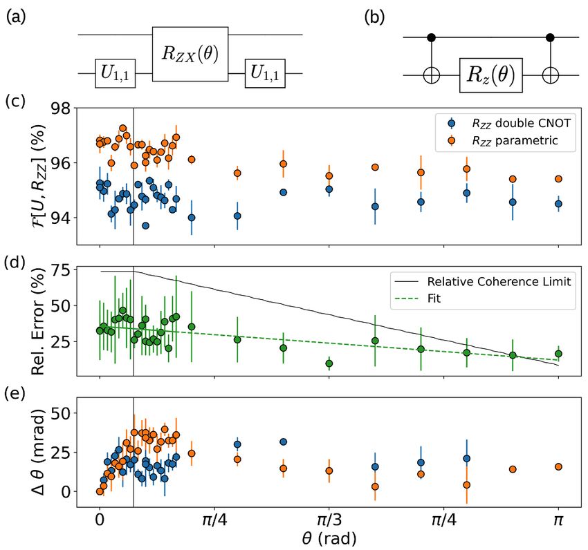
pulse sequence of RZX (π/2) on the control qubit is Figure 1. RZZ (θ) characterization for qubits one and two on
CR(π/4)XCR(−π/4)X. Here, CR(±π/4) are flat-top ibmq_mumbai. (a) Double-CNOT benchmark. √ (b) Continu-
pulses of amplitude A∗ , width w∗ , and Gaussian flanks ous gate implementation where U1,1 = RZ (π/2) XRZ (π/2).
with standard deviations σ, truncated
√ after nσ times σ. Here, RZX (θ) is a scaled cross-resonance pulse with a built-in
Their area is α∗ = |A∗ |[w∗ + 2πσerf(nσ )] where the echo. (c) Gate fidelity F[Umeas , RZZ (θ)] of the double-CNOT
star superscript refers to the parameter values of the cal- implementation (blue) and the scaled cross-resonance pulses
ibrated pulses in the CNOT gate. During each CR pulse (orange). The vertical line indicates the angle at which w = 0.
(d) The relative error between the two implementations (green
rotary tones are applied to the target qubit to help reduce
dots), and the theoretical expectations for a coherence limited
the magnitude of the undesired ωIY interaction. We can gate (solid black line). (e) The deviation angle ∆θ = θ − θmax
create RZX (θ)-rotations by scaling the area of the CR corresponding to the data in (c) that achieves the maximum
and rotary pulses following α(θ) = 2θα∗ /π as done in gate fidelity F[Umeas , RZZ (θmax )].
Ref. [39]. To create a target area α(θ) we first scale w
to minimize the effect of the non-linearity between the
√ ωZX (Ā) and the pulse amplitude. When
drive strength
α(θ) < |A∗ |σ 2πerf(nσ ) we set w = 0√ and scale the pulse
amplitude such that |A(θ)| = α(θ)/[σ 2πerf(nσ )].
We investigate the effect of the pulse scaling method- pendix C. We therefore attribute the error reduction to
ology with quantum process tomography by carefully the shorter schedules as they use less coherence time.
benchmarking scaled RZZ (θ) gates, see Fig. 1(a), with re-
spect to the double-CNOT decomposition, see Fig. 1(b). In addition to the gate fidelity, we compare the de-
We measure the process fidelity F[Umeas , RZZ (θ)] be- viation ∆θ from the target angle of both implemen-
tween the target gate RZZ (θ) and the measured gate tations of the RZZ (θ) rotation. The deviation ∆θ is
Umeas . To determine
√ Umeas we prepare√ each qubit in |0i, the difference between the target rotation angle θ and
|1i, (|0i + |1i)/ 2, and (|0i + i |1i)/ 2 and measure in the angle θmax which satisfies F[Umeas , RZZ (θmax )] ≥
the X, Y , and Z bases. Two qubit process tomography F[Umeas , RZZ (θ0 )] ∀ θ0 . Since the RZ (θ) is virtual [45]
therefore requires a total of 148 circuits for each angle of the implementation with two CNOT gates does not de-
interest which includes four circuits needed to mitigate pend on the desired target angle, see Fig. 1(e). However,
readout errors [15, 16]. The scaled pulses consistently the scaled gate has two competing non-linearities: an ex-
have a better fidelity than the double CNOT benchmark pected non-linearity from the amplitude scaling and an
as demonstrated by the data gathered on ibmq_mumbai unexpected one from scaling the width. As the width is
with qubits one and two, see Fig. 1(c). Appendix B scaled down, the angle deviation increases from ∼10 mrad
shows key device parameters and additional data taken to ∼35 mrad. Once the amplitude scaling begins, a non-
on other IBM Quantum devices which illustrates the re- linearity arises which reduces the √ deviation angle of the
liability of the methodology. The relative error reduc- scaled gates. At α(θ) ≈ |A∗ |σ 2πerf(nσ )/2 the angle
tion of the measured gate fidelity correlates well to the deviation of the scaled gates once again matches the de-
relative error reduction of the coherence limited average viation of the benchmark within the measured standard
gate fidelity [33, 43, 44], see Fig. 1(d) and details in Ap- deviation.3
(a)
q0 : B0 A0 γ
RXX (α) RY Y (β) RZZ (γ) Rel. error reduction (%)
q1 : B1 A1
A3
√ 45 13
q0(b)
7→ 0 : • U1,α • U1,1 • X
q1 7→ 1 : Rz (γ) Rz (β) U2,2
(c)
q0 : H H S† H H S
RZX (α) RZX (β) RZX (γ)
q1 : S† S H H
C β
q0 7→(d)
0: X X A1 A2
RZX ( α2 ) RZX ( −α
2 )
q1 7→ 1 : α
√ Figure 3. Weyl Chamber of SU (4). The coordinates of the
q0 (e)
7→ 0 : U1,1 R X RZX X RZX X RZX U1,0 RZX X RZX X
ZX chamber are O = (0, 0, 0), A1 = (π, 0, 0), A2 = ( π2 , π2 , 0), and
α
(2) ( 2 ) R ( 3π ) ( β2 )
−α
( −β
2 ) U2,1 ( γ2 ) ( −γ
2 ) U1,1
q1 7→ 1 : Z 2 A3 = ( π2 , π2 , π2 ). C corresponds to the CNOT gate. The blue
dots represent the data from Fig. 4 taken on ibmq_mumbai.
Figure 2. Cartan’s KAK decomposition. (a) Circuit rep-
resentation of the KAK decomposition of a two-qubit gate
U ∈ SU (4) with k1 = (A1 ⊗ A0 ) and k2 = (B1 ⊗ B0 ). (b) 60 ibmq_dublin
Circuit in (a) without k1,2 and decomposed into√ three CNOT ibmq_mumbai
50
gates and transpiled to the basis gates (RZ (θ), X, CNOT). Relative error reduction (%)
(c) Circuit in (a) decomposed into the hardware-native RZX 40
gates. Here, each RZX gate has a built-in echo√as shown in (1.86, 1.24, 1.17)
(d). Transpiling circuit (c) to the basis (RZ (θ), X, RZX (θ)) 30
with the echoes exposed to the transpiler results in the pulse-
efficient circuit shown in (e) where the scaled RZX gates do
20
√
√ RZ (nπ/2) XRZ (mπ/2) with
not have an echo. We replaced 10
Un,m and U1,α = RZ (π/2) XRZ (α) to shorten the notation. (0.23, 0.1, 0.06)
0
-10
(1.33, 0.94, 0.79)
III. CREATING ARBITRARY SU(4) GATES 30 40 50 60 70 80 90 100
Relative duration (%)
We now generalize the results from Sec. II. Cartan’s
decomposition of an arbitrary two-qubit gate U ∈ SU (4) Figure 4. Gate error reduction of the pulse-efficient SU (4)
is U = k1 Ak2 which we refer to as Cartan’s KAK gates relative to the three CNOT benchmark for random an-
decomposition [46]. Here k1 and k2 are local opera- gles in the Weyl chamber measured on ibmq_dublin, qubits
T
tions, i.e. k1,2 ∈ SU (2) ⊗ SU (2), and A = eik ·Σ/2 ∈ one and two (light blue circles), and ibmq_mumbai, qubits 19
and 16 (dark blue triangles). The x-axis is the duration of the
SU (4) \ SU (2) ⊗ SU (2) is a non-local operation with
pulse-efficient SU (4) gates relative to the three CNOT bench-
ΣT = (XX, Y Y, ZZ) [47–49], see Fig. 2(a). The non- mark. The angles of three gates are indicated in parenthesis
local term is defined by the three angles kT = (α, β, γ) ∈ as example.
R3 satisfying α + β + γ ≤ 3π/2 and π ≥ α ≥ β ≥ γ ≥ 0.
Geometrically, the KAK decomposition is represented in
a tetrahedron known as the Weyl chamber in the three- duration of the circuit by exposing the echo in the cross-
dimensional space, see Fig. 3. Every point (α, β, γ) in the resonance gate, see Fig. 2(d), to the transpiler. This
Weyl chamber (except in the base) defines a continuous ensures that at most one single-qubit pulse is needed
set of two-qubit gates equivalent up to single-qubit ro- on each qubit between each non-echoed cross-resonance
tations [47]. For instance, the point ( π2 , 0, 0), labeled as RZX gate. By scaling the cross-resonance pulses we cre-
C in Fig. 3, corresponds to the local equivalence class of ate the RZX gates for arbitrary angles and therefore gen-
the CNOT gate, and the point ( π2 , π2 , π2 ), labeled as A3 , eralize the methods of Sec. II to arbitrary gates in SU (4).
represents the SWAP gate. We generate RZX -based circuits as shown in Fig. 2(e)
Since the rotations generated by XX, Y Y , and ZZ for (α, β, γ) angles chosen at random from the Weyl
are locally equivalent to rotations generated by ZX we chamber and measure their fidelity using process to-
T
decompose the non-local eik ·Σ/2 term into a circuit with mography with readout error mitigation. Each RZX -
three RZX rotations, see Fig. 2(c). We shorten the total based circuit is benchmarked against its equivalent three4
(a) q0 : • • • • (b) q0 : • • (d) q0 :
Rzz (−θ) Rzz (1) Rzz (3)
q1 : RZ (1) RZ (−2) × RZ (3) q1 : RZ (θ) q1 :
SWAP (−2)
q2 : • • × q2 :
(c) q0 : • • ×
SWAP (−θ)
q1 : RZ (θ) ×
(e)
q0 7→ 0 : X X X X
RZX ( −1
2 ) RZX ( 12 ) RZX ( −3
2 ) RZX ( 23 )
q1 7→ 1 : U1,1 U1,1 RZ ( 3π
2)
U2,1 U1,1
RZX ( π4 ) RZX ( −π
4 ) √ RZX ( π4 ) RZX ( −π
4 ) RZX (−c) RZX (c)
q2 7→ 2 : U1,1 X X X U1,0 X X
Figure 5. Pulse-efficient transpilation example. (a) Circuit of the cost operator for a QAOA circuit implemented on three qubits
connected in a line. (b) and (c) Templates of the RZZ and phase-swap gates, respectively. Here, RZZ (θ) and SWAP(θ) hold
the rules with which to decompose them into the hardware-native RZX gates. (d) Circuit resulting from the template matching
of (b) and (c) performed on circuit (a). (e) Circuit resulting from a transpilation of (d)
√ which uses the decompositions rules of
RZZ (θ) and SWAP(θ) into RZX . To shorten the circuit figure we replaced RZ (nπ/2) XRZ (mπ/2) with Un,m and c = 0.215.
CNOT decomposition presented in Ref. [50] and shown in is
Fig. 2(b). The experiments are run on ibmq_dublin and
ibmq_mumbai with 2048 shots for each circuit which we O |C||T |+3 |T ||T |+4 nnCT −1 , (2)
measure three times to gain statistics. The pulse-efficient
RZX -based decomposition of the circuits results in a sig- i.e. exponential in the template length [52]. We therefore
nificant fidelity increase for almost all angles, see Fig. 4. create short templates where the inverse of the intended
A subset of the data is also shown in the Weyl chamber †
match, i.e. Umatch , is specified as a single gate with rules
in Fig. 3. The correlation between the relative error re- to further decompose it into RZX and single-qubit gates
duction and the relative schedule duration indicates that in a subsequent transpilation pass. In these decompo-
the gains in fidelity come from a better usage of the fi- sitions we expose the echoed cross-resonance implemen-
nite coherence time as the scaled cross-resonance pulses tation of RZX to the transpiler by writing RZX (θ) =
achieve the same unitary in less time. Remarkably, these XRZX (−θ/2)XRZX (θ/2). This allows the transpiler to
results were achieved without recalibrating any pulses. further simplify the single-qubit gates that would other-
wise be hidden in the schedules of the two-qubit gates, as
exemplified in the circuit in Fig. 5(e). Finally, once the
RZX (θ) gates are introduced into the quantum circuit we
IV. PULSE-EFFICIENT TRANSPILER PASSES run a third transpilation pass to attach pulse schedules
to each RZX (θ) gate built from the backend’s calibrated
The quantum circuits of an algorithm are typically CNOT gates following the procedure in Sec. II. The at-
expressed using generic gates such as the CNOT or tached schedules consist of the scaled cross-resonance
controlled-phase gate and then transpiled to the hard- pulse and rotary tone without any echo. Details on the
ware on which they are run [51]. Quantum algorithms Qiskit implementation are given in Appendix A.
can benefit from the continuous family of gates presented
in Sec. II and III if the underlying quantum circuit is ei-
ther directly built from, or transpiled to, the hardware V. IMPROVING QAOA WITH CARTAN’S
native RZX (θ) gate. We now show how to transpile DECOMPOSITION
quantum circuits to a RZX (θ)-based-circuit with tem-
plate substitution [52]. We use the QAOA [4, 53, 54], applied to MAXCUT,
A template is a quantum circuit made of |T | gates act- to demonstrate gains of a pulse-efficient circuit transpi-
ing on nT qubits that compose to the identity U1 ...U|T | = lation on noisy hardware. QAOA maps a quadratic bi-
1, see e.g. Fig. 5(b) and (c). In a template substi- nary optimization problem with n decision
P variables to
tution transpilation pass we identify a sub-set of the a cost function Hamiltonian ĤC = i,j αi,j Zi Zj where
gates in the template Ua ...Ub that match those in a given αij ∈ R are problem dependent and Zi are Pauli Z
quantum circuit. Next, if a cost of the matched gates operators. The ground state of ĤC encodes the so-
is higher than the cost of the unmatched gates in the lution to the problem. Next, a classical solver mini-
template we replace Umatch = Ua ...Ub with Umatch = mizes the energy hψ(β, γ)|ĤC |ψ(β, γ)i of a trial state
†
Ua−1 ...U1† U|T
† †
| ...Ub+1 . As cost we use a heuristic that
|ψ(β, γ)i created by applying p-layers of the operator
Pj−n
sums the cost of each gate defined as an integer weight exp(−iβk i=0 Xj ) exp(−iγk ĤC ) where k = 1, ..., p to
which is higher for two-qubit gates, details are provided the equal superposition of all states.
in Appendix A. The complexity of the template match- Implementing the operator exp(−iγk ĤC ) requires ap-
ing algorithm on a circuit with |C| gates and nC qubits plying the RZZ (θ) = exp(−iθZZ/2) gate on pairs of5
(a) (b) 3
0
1 queue of the cloud-based IBM Quantum computers. For
2
4
2
5
1 each (β, γ) pair we run the circuits with the noiseless
1 1
1 3 1
QASM simulator in Qiskit, see Fig. 6(a) and twice on
2
3 1 2 3
3
the hardware. The first hardware run is done using a
3 8
2
1 1
6
CNOT decomposition with the Qiskit transpiler on opti-
1 7 2 mization level three, see Fig. 6(c) for results. The second
9 10
1
run is done with the pulse-efficient circuit transpilation,
(c) (d) see Fig. 6(e) for results. Here, we first perform the tem-
plate substitution with the RZZ (θ) and SWAP(θ) tem-
plates, shown in Fig. 5(b), (c) and Appendix A for fur-
ther details. A second transpilation pass then exposes
the RZX (θ) gates to which we attach pulse schedules
in a third transpilation pass following Sections II – IV.
In each case we measure 4096 shots. The pulse-efficient
(e) (f) circuits produce less noisy average cut values, compare
Fig. 6(c) with (e), and have a lower absolute deviation
from the noiseless simulation than the circuits transpiled
to CNOT gates, compare Fig. 6(d) with (f). The max-
imum error in the cut value averaged over the sampled
bit-strings is reduced by 38% from 3.65 to 2.26. We at-
tribute the increased quality of the results to the decrease
in total cross-resonance time and the fact that the pulse-
efficient transpilation keeps the number of single-qubit
Figure 6. Depth-one QAOA energy landscape. (a) Noiseless pulses to a minimum. In total, we observe a reduction
simulation of the cut value, averaged over all 4096 bit-strings in total schedule duration ranging from 42% to 52% de-
sampled from |ψ(β, γ)i, obtained using the QASM simulator pending on γ when using the pulse efficient transpilation
for the weighted graph shown in (b). The maximum cut, with
methodology, see Fig. 7. Since the schedule duration of
value 28, is indicated by the color of the nodes in (b). Figures
(c) and (e) show hardware results obtained by transpiling to
RZZ (γαi,j ) and SWAP(γαi,j ) decreases and increases as
CNOT gates and by using the RZX pulse-efficient method- γ decreases, respectively, we observe a non-monotonous
ology, respectively. Figures (d) and (f) share the same color reduction in the schedule duration of the QAOA circuit
scale and show the absolute deviation from the ideal averaged as a function of γ.
cut values in figures (c) and (e), respectively.
qubits. However, to overcome the limited connectivity of
Reduction (%) Schedule duration ( s)
superconducting qubit chips [55], several RZZ (θ) gates 8
are followed or preceded by a SWAP resulting in the uni-
(a) CNOT basis Pulse-efficient
tary operator 6
1 0 0 0
0 0 eiθ 0 4
SWAP(θ) = (3)
0 eiθ 0 0 1.00 0.75 0.50 0.25 0.00 0.25 0.50 0.75 1.00
0 0 0 1 55
50 (b)
up to a global phase. When mapped to the KAK decom-
45
position SWAP(θ) corresponds to kT = (ηπ/2, ηπ/2, θ +
ηπ/2)) where η = −1 if θ > 0 and 1 otherwise. This al- 40 1.00 0.75 0.50 0.25 0.00 0.25 0.50 0.75 1.00
lows us to reduce the total cross-resonance duration using (rad)
the methodology presented in Sec. III.
We perform a depth-one QAOA circuit for an eleven Figure 7. QAOA schedule durations. (a) Duration of the
node graph, shown in Fig. 6(b), built from CNOT gates. scheduled quantum circuits transpiled to CNOTs with opti-
We map the decision variables zero to ten to qubits 7, mization level three (blue circles) and with the pulse-efficient
10, 12, 15, 18, 13, 8, 11, 14, 16, 19 on ibmq_mumbai, re- methodology (orange triangles). In both cases we removed the
final measurements from the quantum circuits. (b) Length
spectively. Since the graph is non-hardware-native eight
of the pulse efficient schedules relative to the CNOT-based
SWAP gates are needed to implement the circuits. In schedules.
QAOA the optimal values of (β, γ) are found with a clas-
sical optimizer [56]. Here, we scan β and γ from ±2 rad
and ±1 rad, respectively, as we submit jobs through the6
VI. DISCUSSION AND CONCLUSION and benchmarking their impact on Quantum Volume [8].
Methods to interpolate pulse parameters based on a set
of reference RZX (θ) gates, calibrated at a few reference
The results in Sec. II and III showed that by scal- angles θ, might also improve the gate fidelity and help
ing cross-resonance gates we can automatically create deal with non-linearities between the rotation angle θ and
a continuous family of gates which implements SU (4). pulse parameters. For variational algorithms, such as the
These scaled gates typically have shorter pulse schedules variational quantum eigensolver, the scaled SU (4) gates
and higher fidelities than the digital CNOT implementa- may allow for better results due to the shorted schedules
tion. This fidelity is limited by coherence, imperfections while still being robust to some unitary errors such as
in the initial calibration, and non-linear effects. Cru- angle errors [58, 59].
cially, the resulting gate-tailored pulse schedules do not We believe that the methods presented in our work
require additional calibration and can therefore be au- will help users of noisy quantum hardware to reap the
tomatically generated by the transpiler. Transpilation benefits of pulse-level control without having to know
passes, as discussed in Sec. IV, can be leveraged to iden- its intricacies. This can improve the quality of a broad
tify and attach the scaled pulse schedules to the gates class of quantum applications running on noisy quantum
in a quantum circuit. Furthermore, exposing the echo hardware.
in the cross-resonance gate to the transpiler allows fur-
ther simplifications of the single-qubit gates. We used
this pulse-efficient transpilation methodology to reduce VII. ACKNOWLEDGMENTS
errors in an eleven-qubit depth-one QAOA.
The authors acknowledge use of the IBM Quantum de-
Scaled gates are particularly appealing for Trotter vices for this work. The authors also thank L. Capelluto,
based applications, as shown in Ref. [39], and could N. Kanazawa, N. Bronn, T. Itoko and E. Pritchett for
therefore benefit quantum simulations [57]. Future work insightful discussions and S. Woerner for a careful read
may also include scaling direct cross-resonance gates [9] of the manuscript.
[1] Nikolaj Moll, Panagiotis Barkoutsos, Lev S. Bishop, A 100, 032328 (2019).
Jerry M. Chow, Andrew Cross, Daniel J. Egger, Ste- [9] Petar Jurcevic, Ali Javadi-Abhari, Lev S. Bishop, Isaac
fan Filipp, Andreas Fuhrer, Jay M. Gambetta, Marc Lauer, Daniela F. Bogorin, Markus Brink, Lauren Capel-
Ganzhorn, and et al., “Quantum optimization using luto, Oktay Günlük, Toshinari Itoko, Naoki Kanazawa,
variational algorithms on near-term quantum devices,” and et al., “Demonstration of quantum volume 64 on a
Quantum Sci. Technol. 3, 030503 (2018). superconducting quantum computing system,” Quantum
[2] Román Orús, Samuel Mugel, and Enrique Lizaso, Sci. Technol. 6, 025020 (2021).
“Quantum computing for finance: Overview and [10] Philip Krantz, Morten Kjaergaard, Fei Yan, Terry P. Or-
prospects,” Rev. Phys. 4, 100028 (2019). lando, Simon Gustavsson, and William D. Oliver, “A
[3] Daniel J. Egger, Claudio Gambella, Jakub Marecek, quantum engineer’s guide to superconducting qubits,”
Scott McFaddin, Martin Mevissen, Rudy Raymond, Aan- Appl. Phys. Rev. 6, 021318 (2019).
drea Simonetto, Sefan Woerner, and Elena Yndurain, [11] Morten Kjaergaard, Mollie E. Schwartz, Jochen
“Quantum computing for finance: State-of-the-art and Braumüller, Philip Krantz, Joel I.-J. Wang, Simon
future prospects,” IEEE Transactions on Quantum Engi- Gustavsson, and William D. Oliver, “Superconducting
neering 1, 1–24 (2020). qubits: Current state of play,” Annu. Rev. Condens. Mat-
[4] Edward Farhi, Jeffrey Goldstone, and Sam Gutmann, “A ter Phys. 11, 369–395 (2020).
quantum approximate optimization algorithm,” (2014), [12] Jens Koch, Terri M. Yu, Jay M. Gambetta, Andrew A.
arXiv:1411.4028 [quant-ph]. Houck, David I. Schuster, Johannes Majer, Alexan-
[5] Daniel J. Egger, Jakub Marecek, and Stefan Wo- dre Blais, Michel H. Devoret, Steven M. Girvin, and
erner, “Warm-starting quantum optimization,” (2020), Robert J. Schoelkopf, “Charge-insensitive qubit design
arXiv:2009.10095 [quant-ph]. derived from the cooper pair box,” Phys. Rev. A 76,
[6] Jacob Biamonte, Peter Wittek, Nicola Pancotti, Patrick 042319 (2007).
Rebentrost, Nathan Wiebe, and Seth Lloyd, “Quantum [13] Chad Rigetti, Jay M. Gambetta, Stefano Poletto, Brit-
machine learning,” Nature 549, 195–202 (2017). ton L. T. Plourde, Jerry M. Chow, Antonio D. Córcoles,
[7] Vojtech Havlicek, Antonio D. Corcoles, Kristan Temme, John A. Smolin, Seth T. Merkel, Jim R. Rozen, George A.
Aram W. Harrow, Abhinav Kandala, Jerry M. Chow, Keefe, and et al., “Superconducting qubit in a waveguide
and Jay M. Gambetta, “Supervised learning with cavity with a coherence time approaching 0.1 ms,” Phys.
quantum-enhanced feature spaces,” Nature 567, 209 – Rev. B 86, 100506 (2012).
212 (2019). [14] IBM Quantum, https://quantum-computing.ibm.com/
[8] Andrew W. Cross, Lev S. Bishop, Sarah Sheldon, Paul D. (2021).
Nation, and Jay M. Gambetta, “Validating quantum [15] Sergey Bravyi, Sarah Sheldon, Abhinav Kandala,
computers using randomized model circuits,” Phys. Rev. David C. Mckay, and Jay M. Gambetta, “Mitigating7
measurement errors in multi-qubit experiments,” (2020), [28] Adriaan M. Rol, Cornelis C. Bultink, Thomas E.
arXiv:2006.14044 [quant-ph]. O’Brien, S. R. de Jong, Lukas S. Theis, Xiang Fu,
[16] George S. Barron and Christopher J. Wood, “Measure- F. Luthi, Raymond F. L. Vermeulen, J. C. de Sterke,
ment error mitigation for variational quantum algo- Alessandro Bruno, and et al., “Restless tuneup of
rithms,” (2020), arXiv:2010.08520 [quant-ph]. high-fidelity qubit gates,” Phys. Rev. Applied 7, 041001
[17] Kristan Temme, Sergey Bravyi, and Jay M. Gam- (2017).
betta, “Error mitigation for short-depth quantum cir- [29] Max Werninghaus, Daniel J. Egger, and Stefan Fil-
cuits,” Phys. Rev. Lett. 119, 180509 (2017). ipp, “High-speed calibration and characterization of su-
[18] Abhinav Kandala, Kristan Temme, Antonio D. Corcoles, perconducting quantum processors without qubit reset,”
Antonio Mezzacapo, Jerry M. Chow, and Jay M. Gam- (2020), arXiv:2010.06576 [quant-ph].
betta, “Error mitigation extends the computational reach [30] Shai Machnes, Elie Assémat, David Tannor, and
of a noisy quantum processor,” Nature 567, 491–495 Frank K. Wilhelm, “Tunable, flexible, and efficient op-
(2018). timization of control pulses for practical qubits,” Phys.
[19] Nathan Lacroix, Christoph Hellings, Christian Kraglund Rev. Lett. 120, 150401 (2018).
Andersen, Agustin Di Paolo, Ants Remm, Stefania [31] Jerry M. Chow, Antonio D. Córcoles, Jay M. Gambetta,
Lazar, Sebastian Krinner, Graham J. Norris, Mihai Chad Rigetti, Blake R. Johnson, John A. Smolin, Jim R.
Gabureac, Johannes Heinsoo, and et al., “Improving the Rozen, George A. Keefe, Mary B. Rothwell, Mark B.
performance of deep quantum optimization algorithms Ketchen, and M. Steffen, “Simple all-microwave entan-
with continuous gate sets,” PRX Quantum 1, 110304 gling gate for fixed-frequency superconducting qubits,”
(2020). Phys. Rev. Lett. 107, 080502 (2011).
[20] Brooks Foxen, Charles Neill, Andrew Dunsworth, Pe- [32] Sarah Sheldon, Easwar Magesan, Jerry M. Chow, and
dram Roushan, Ben Chiaro, Anthony Megrant, Julian Jay M. Gambetta, “Procedure for systematically tuning
Kelly, Zijun Chen, Kevin J. Satzinger, Rami Barends, up cross-talk in the cross-resonance gate,” Phys. Rev. A
and et al. (Google AI Quantum), “Demonstrating a con- 93, 060302 (2016).
tinuous set of two-qubit gates for near-term quantum al- [33] Neereja Sundaresan, Isaac Lauer, Emily Pritchett,
gorithms,” Phys. Rev. Lett. 125, 120504 (2020). Easwar Magesan, Petar Jurcevic, and Jay M. Gambetta,
[21] Pranav Gokhale, Ali Javadi-Abhari, Nathan Earnest, “Reducing unitary and spectator errors in cross resonance
Yunong Shi, and Frederic T Chong, “Optimized quan- with optimized rotary echoes,” PRX Quantum 1, 020318
tum compilation for near-term algorithms with open- (2020).
pulse,” in 2020 53rd Annual IEEE/ACM International [34] David C. McKay, Thomas Alexander, Luciano Bello,
Symposium on Microarchitecture (MICRO) (IEEE, 2020) Michael J. Biercuk, Lev Bishop, Jiayin Chen, Jerry M.
pp. 186–200. Chow, Antonio D. Córcoles, Daniel J. Egger, Ste-
[22] Navin Khaneja, Timo Reiss, Cindie Kehlet, Thomas fan Filipp, and et al., “Qiskit backend specifications
Schulte-Herbrüggen, and Steffen J. Glaser, “Optimal for openqasm and openpulse experiments,” (2018),
control of coupled spin dynamics: design of nmr pulse arXiv:1809.03452 [quant-ph].
sequences by gradient ascent algorithms,” J. Magn. Re- [35] Thomas Alexander, Naoki Kanazawa, Daniel J. Egger,
son. 172, 296–305 (2005). Lauren Capelluto, Christopher J. Wood, Ali Javadi-
[23] Yunong Shi, Nelson Leung, Pranav Gokhale, Zane Rossi, Abhari, and David C. McKay, “Qiskit pulse: program-
David I. Schuster, Henry Hoffmann, and Frederic T. ming quantum computers through the cloud with pulses,”
Chong, “Optimized compilation of aggregated instruc- Quantum Sci. Technol. 5, 044006 (2020).
tions for realistic quantum computers,” in Proceedings of [36] Shelly Garion, Naoki Kanazawa, Haggai Landa, David C.
the Twenty-Fourth International Conference on Architec- McKay, Sarah Sheldon, Andrew W. Cross, and Christo-
tural Support for Programming Languages and Operating pher J. Wood, “Experimental implementation of non-
Systems, ASPLOS ’19 (Association for Computing Ma- clifford interleaved randomized benchmarking with a
chinery, New York, NY, USA, 2019) pp. 1031–1044. controlled-s gate,” Phys. Rev. Research 3, 013204 (2021).
[24] Daniel J. Egger and Frank K. Wilhelm, “Adaptive hy- [37] Shun Oomura, Takahiko Satoh, Michihiko Sugawara,
brid optimal quantum control for imprecisely character- and Naoki Yamamoto, “Design and application of high-
ized systems,” Phys. Rev. Lett. 112, 240503 (2014). speed and high-precision cv gate on ibm q openpulse sys-
[25] Nicolas Wittler, Federico Roy, Kevin Pack, Max Wern- tem,” (2021), arXiv:2102.06117 [quant-ph].
inghaus, Anurag Saha Roy, Daniel J. Egger, Stefan Fil- [38] Kentaro Heya and Naoki Kanazawa, “Cross cross reso-
ipp, Frank K. Wilhelm, and Shai Machnes, “Integrated nance gate,” (2021), arXiv:2103.00024 [quant-ph].
tool set for control, calibration, and characterization [39] John P. T. Stenger, Nicholas T. Bronn, Daniel J. Egger,
of quantum devices applied to superconducting qubits,” and David Pekker, “Simulating the dynamics of braid-
Phys. Rev. Applied 15, 034080 (2021). ing of majorana zero modes using an ibm quantum com-
[26] Julian Kelly, Rami Barends, Brooks Campbell, Yu Chen, puter,” (2021), arXiv:2012.11660 [quant-ph].
Zijun Chen, Ben Chiaro, Andrew Dunsworth, Austin G. [40] Masoud Mohseni, Ali T. Rezakhani, and Daniel A. Li-
Fowler, IoChun Hoi, Evan Jeffrey, and et al., “Opti- dar, “Quantum-process tomography: Resource analysis
mal quantum control using randomized benchmarking,” of different strategies,” Phys. Rev. A 77, 032322 (2008).
Phys. Rev. Lett. 112, 240504 (2014). [41] Radoslaw C. Bialczak, Markus Ansmann, Max Hofheinz,
[27] Max Werninghaus, Daniel J. Egger, Federico Roy, Shai Erik Lucero, Matthew Neeley, Aaron D. O’Connell,
Machnes, Frank K. Wilhelm, and Stefan Filipp, “Leakage Daniel Sank, Haohua Wang, Jim Wenner, Matthias Stef-
reduction in fast superconducting qubit gates via optimal fen, and et al., “Quantum process tomography of a uni-
control,” npj Quantum Inf. 7, 14 (2021). versal entangling gate implemented with josephson phase
qubits,” Nat. Phys. 6, 409–413 (2010).8
[42] Easwar Magesan and Jay M. Gambetta, “Effective hamil- [58] James I. Colless, Vinay V. Ramasesh, Dar Dahlen,
tonian models of the cross-resonance gate,” Phys. Rev. A Machiel S. Blok, Mollie E. Kimchi-Schwartz, Jarrod R.
101, 052308 (2020). McClean, Jonathan Carter, Wibe A. de Jong, and Irfan
[43] Michał Horodecki, Paweł Horodecki, and Ryszard Siddiqi, “Computation of molecular spectra on a quan-
Horodecki, “General teleportation channel, singlet frac- tum processor with an error-resilient algorithm,” Phys.
tion, and quasidistillation,” Phys. Rev. A 60, 1888–1898 Rev. X 8, 011021 (2018).
(1999). [59] Daniel J. Egger, Marc Ganzhorn, Gian Salis, Andreas
[44] Easwar Magesan, Robin Blume-Kohout, and Joseph Fuhrer, Peter Müller, Panagiotis Kl. Barkoutsos, Nikolaj
Emerson, “Gate fidelity fluctuations and quantum pro- Moll, Ivano Tavernelli, and Stefan Filipp, “Entanglement
cess invariants,” Phys. Rev. A 84, 012309 (2011). generation in superconducting qubits using holonomic
[45] David C. McKay, Christopher J. Wood, Sarah Sheldon, operations,” Phys. Rev. Applied 11, 014017 (2019).
Jerry M. Chow, and Jay M. Gambetta, “Efficient z
gates for quantum computing,” Phys. Rev. A 96, 022330
(2017).
[46] Navin Khaneja and Steffen J. Glaser, “Cartan decom-
position of SU(2n ) and control of spin systems,” Chem.
Phys. 267, 11–23 (2001).
[47] Jun Zhang, Jiri Vala, Shankar Sastry, and Birgitta K.
Whaley, “Geometric theory of nonlocal two-qubit opera-
tions,” Phys. Rev. A 67, 042313 (2003).
[48] Robert R. Tucci, “An introduction to cartan’s kak de-
composition for qc programmers,” (2005), arXiv:quant-
ph/0507171.
[49] Byron Drury and Peter Love, “Constructive quantum
shannon decomposition from cartan involutions,” J.
Phys. A: Math. Theor. 41, 395305 (2008).
[50] Guifre Vidal and Christopher M. Dawson, “Universal
quantum circuit for two-qubit transformations with three
controlled-not gates,” Phys. Rev. A 69, 010301 (2004).
[51] Héctor Abraham, AduOffei, Rochisha Agarwal, Is-
mail Yunus Akhalwaya, Gadi Aleksandrowicz, Thomas
Alexander, Matthew Amy, Eli Arbel, Arijit02, Abraham
Asfaw, and et al., “Qiskit: An open-source framework
for quantum computing,” (2019).
[52] Raban Iten, Romain Moyard, Tony Metger, David Sut-
ter, and Stefan Woerner, “Exact and practical pattern
matching for quantum circuit optimization,” (2020),
arXiv:1909.05270 [quant-ph].
[53] Edward Farhi, Jeffrey Goldstone, and Sam Gutmann,
“A quantum approximate optimization algorithm applied
to a bounded occurrence constraint problem,” (2015),
arXiv:1412.6062 [quant-ph].
[54] Zhi-Cheng Yang, Armin Rahmani, Alireza Shabani,
Hartmut Neven, and Claudio Chamon, “Optimizing vari-
ational quantum algorithms using pontryagin’s minimum
principle,” Phys. Rev. X 7, 021027 (2017).
[55] Matthew P. Harrigan, Kevin J. Sung, Matthew Neeley,
Kevin J. Satzinger, Frank Arute, Kunal Arya, Juan Ata-
laya, Joseph C. Bardin, Rami Barends, Sergio Boixo, and
et al., “Quantum approximate optimization of non-planar
graph problems on a planar superconducting processor,”
Nat. Phys. 17, 332–336 (2021).
[56] Andreas Bengtsson, Pontus Vikstål, Christopher War-
ren, Marika Svensson, Xiu Gu, Anton Frisk Kockum,
Philip Krantz, Christian Križan, Daryoush Shiri, Ida-
Maria Svensson, and et al., “Improved success proba-
bility with greater circuit depth for the quantum approx-
imate optimization algorithm,” Phys. Rev. Applied 14,
034010 (2020).
[57] Sabine Tornow, Wolfgang Gehrke, and Udo Helmbrecht,
“Non-equilibrium dynamics of a dissipative two-site hub-
bard model simulated on the ibm quantum computer,”
(2020), arXiv:2011.11059 [quant-ph].9
Appendix A: Qiskit implementation # 1. Template substitution: introduces custom
# gates with an rzx decomposition
Quantum circuits often have repeating sub-circuits pass_ = TemplateOptimization(
with different parameters. For instance, QAOA circuits template_list=[swap(), rzz()],
include many RZZ (γαij ) and SWAP(γαij ) gates where γ user_cost_dict=cost_dict)
is one of the variational parameters and the {αij } depend
on the problem instance. We therefore need parametric qct = PassManager(pass_).run(qc)
templates when running the template substitution algo-
rithm. # 2. Unroll to rzx basis and simplify gates
gates = ['rz', 'sx', 'rzx', 'cx', 'x']
(a) q0 : RZ (−θ) • •
qct_rzx = transpile(qct,
CZ(2θ) backend,
q1 : RZ (−θ) RZ (θ)
optimization_level=1,
basis_gates=gates)
(b) q0 : RZ (−2) • •
# 3. Add custom rzx pulse schedules
q1 : RZ (−2) RZ (2) RZ (3) • •
pass_ = RZXCalibrationBuilderNoEcho(backend)
q2 : RZ (3) RZ (3) cal_qc = PassManager(pass_).run(qct_rzx)
Figure 9. Example of a circuit transpilation that achieves a
Figure 8. (a) Parametric template of a controlled-Z gate. (b) pulse-efficient circuit transpilation.
Circuit on which the template matching is run. The dashed
blue and dotted purple boxes indicate potential matches based
on circuit instruction names and qubits. RZXCalibrationBuilderNoEcho class scales the pulses
of the cross-resonance gates and attaches them to the
We extended the Qiskit implementation of Ref. [52] to RZX (θ) gates in the circuit. Figure 10 exemplifies the
parametric templates. To avoid a symbolic description result of the first transpilation pass applied to the QAOA
of the unitary matrix of each gate we first match gates circuit in Sec. V.
by qubits and name. This is however not sufficient to
q0 : H RX (−2)
create a valid match since, for example, the parametric q1 : H
SWAP (1)
RX (−2)
template in Fig. 8(a) produces two tentative matches on q2 : H
RZZ (1) RZZ (2) RZZ (3)
RX (−2)
RZZ (1) SWAP (2)
the circuit in Fig. 8(b). We therefore form a system of q3 : H
SWAP (1) SWAP (1) RZZ (3) RZZ (3)
RX (−2)
q4 : H RX (−2)
equations based on the tentative match. If this system
q5 : H RX (−2)
of equations accepts a solution the match is valid. For q6 : H RX (−2)
RZZ (1) RZZ (1) SWAP (2) SWAP (2)
example, the tentative match in Fig. 8(b), indicated by q7 : H RX (−2)
SWAP (1) RZZ (3)
the dashed blue box, results in the system of equations q8 : H
RZZ (1) RZZ (2) RZZ (3)
RX (−2)
q9 : H RX (−2)
SWAP (1)
q10 : H RX (−2)
−θ = −2
−θ = −2 (A1)
θ=2
Figure 10. 11 qubit QAOA circuit with γ = 1 and β =
−2 after the template substitution. The final measurement
which accepts the solution θ = 2 and is therefore valid. instructions have been omitted.
However, the second tentative match, highlighted by the
dotted purple box, results in the system of equations The template optimization pass requires a cost
dictionary to determine if it is favourable to replace
−θ = 3
the matched gates Umatch = Ua ...Ub from a template
−θ = 3 (A2) with the Hermitian conjugate of the remaining part of
†
the template Ua−1 ...U1† U|T
† †
| ...Ub+1 . The cost dictionary
θ=3
has gates as keys and their cost as value. The cost of
which has no solution and is therefore not valid. Ua ...Ub is the sum of the costs of each individual gate Ua
We achieve a pulse-efficient circuit transpilation with to Ub . We used the cost dictionary {’sx’: 1, ’x’:
Qiskit by using three transpilation steps shown in 1, ’rz’: 0, ’cx’: 2, ’rzz’: 0, ’swap’: 6,
Fig. 9. First, the TemplateOptimization transpila- ’phase_swap’: 0} which assigns a zero cost to the
tion pass is applied with the SWAP and rzz templates rzz and phase_swap gates which correspond to the
as shown in Fig. 5(b) and (c) of the main text. The pulse-efficient implementation of RZZ (θ) and SWAP(θ).
next step, a standard transpiler pass with a low op- Single-qubit gates have unit cost except for rz which is
timization level, i.e. one, exposes the rzx definition implemented with virtual Z-rotations. The CNOT gate,
of the gates in the matched templates. Finally, the i.e. cx, and the standard SWAP gate, i.e. swap have10
costs two and six, respectively. This cost dictionary en- Appendix C: Theoretical coherence limit
sures that the template substitution will include RZZ (θ)
and SWAP(θ) in the case of a match. Future work could In Sections II we compared the relative decrease in gate
improve this heuristic cost dictionary either by using the error to the coherence limit on the average gate error E.
fidelity of the gates (if this metric is available) or the This limit is implemented in Qiskit Ignis for two qubits
duration of the underlying pulse schedules as cost. a and b as E = 43 (1 − u1 − u2 ) where
1 −t/T1,a
u1 = e + e−t/T1,b + e−t/T1,a −t/T1,b , (C1)
Appendix B: Properties of the Quantum devices and 15
additional data 2 −t/T2,b
u2 = e + e−t/T2,b −t/T1,a + e−t/T2,a (C2)
15
Since the qubit coherence times as well as the CNOT + e−t/T2,a −t/T1,b + 2e−t/T2,a −t/T2,b .
gate duration and error mainly limit the fidelity of the
scaled cross-resonance gates we list their values for the The derivation of this limit is discussed in more detail
qubits and devices we experimented with in Tab. I. To in Appendix G of Ref. [33]. Here, t is the gate duration
illustrate that scaling imperfect cross-resonance gates im- while T1,a and T2,a are the T1 and T2 times for qubit
proves the gate fidelity we measured the process fidelity a. Since the process fidelity and the average gate fidelity
on several IBM Quantum devices and qubit pairs. In are linearly related [43, 44] we compare the relative er-
almost all measurements the scaled gates have a higher ror reduction in the measured process fidelity with the
fidelity than the double CNOT benchmark and the rel- theoretical relative error reduction in E.
ative error reduction increases as the schedule duration
decreases, see Fig. 11.
Table I. Summary of the properties of the CNOT gates and
coherence times for the qubits used to benchmark the perfor-
mance of the scaled cross-resonance gates.
CNOT
Device error duration T1 -times T2 -times
(%) (ns) (µs) (µs)
ibmq_mumbai
q1, q2 1.27 739 102, 157 34, 228
q16, q19 0.84 754 84, 141 105, 132
ibmq_paris
q1, q2 1.70 597 66, 92 82, 128
q13, q14 1.28 434 100, 23 27, 33
q18, q15 5.36 448 86, 74 103, 50
q18, q17 1.76 725 41, 71 94, 157
ibmq_dublin
q1, q2 0.76 540 110, 103 174, 89
q3, q2 0.83 370 78, 96 100, 83
ibmq_montreal
q14, q16 0.88 356 97, 87 97, 52
ibmq_guadalupe
q7, q10 0.61 299 99, 68 153, 90
Fig. 12 shows additional quantum process tomography
results for Cartan-decomposed circuits chosen at random
in the Weyl chamber. The experiments were performed
on ibmq_dublin, see Fig. 12(a), and ibmq_paris using
different qubit pairs, see Fig. 12(b) – (d). For almost
all angles the relative error reduction is positive which
demonstrates the advantage of a hardware-native, scaled
cross-resonance gate based circuit implementation.11
(a) 98.0 (b) 99.0
97.5 RZZ double CNOT 98.5 RZZ double CNOT
Fidelity (%) 97.0 RZZ scaled CR 98.0 RZZ scaled CR
Fidelity (%)
96.5 97.5
96.0 97.0
95.5
95.0 96.5
94.5 96.0
75 75
Reduction (%)
Reduction (%)
Relative Error
Relative Error
50 50
25 25
0 0 /4 /2 3 /4 0 0 /4 /2 3 /4
(rad) (rad)
(c) 98.0 (d) 99.0
RZZ double CNOT 98.5 RZZ double CNOT
97.0 RZZ scaled CR RZZ scaled CR
98.0
Fidelity (%)
Fidelity (%)
96.0 97.5
95.0 97.0
94.0 96.5
96.0
93.0 95.5
75 75
Reduction (%)
Reduction (%)
Relative Error
Relative Error
50 50
25 25
0
0 -25
0 /4 /2 3 /4 0 /4 /2 3 /4
(rad) (rad)
Figure 11. Gate fidelity measured with quantum process tomography and relative error reduction for the ZZ-gate as a function
of θ on ibmq_mumbai (qubits 16 and 19), ibmq_montreal (qubits 14 and 16), ibmq_paris (qubits 1 and 2) and ibmq_guadalupe
(qubits 7 and 10). (a-d, top) Process fidelities for the RZZ double CNOT (blue up-triangles) and scaled CR (orange down-
triangles) circuit implementation. (a-d, bottom) Relative error reduction calculated from the fidelities.12
(a) (b)
50 100
Relative error reduction (%)
Relative error reduction (%)
40
80
30
20 60
10 40
0
20
-10
-20 55 60 65 70 75 80 85 50 55 60 65 70 75 80 85
Relative duration (%) Relative duration (%)
(c) (d)
40
30
Relative error reduction (%)
Relative error reduction (%)
30 25
20 20
15
10
10
0 5
-10 0
50 60 70 80 90 60 65 70 75 80 85
Relative duration (%) Relative duration (%)
Figure 12. Quantum Process Tomography results for random angles in the Weyl chamber on (a) ibmq_dublin (qubits 3 and
2), (b) ibmq_paris (qubits 18 and 15), (c) ibmq_paris (qubits 13 and 14) and (d) ibmq_paris (qubits 18 and 17).You can also read