The cyclic expansion and contraction characteristics of a loess slope and implications for slope stability - Nature
←
→
Page content transcription
If your browser does not render page correctly, please read the page content below
www.nature.com/scientificreports
OPEN The cyclic expansion
and contraction characteristics
of a loess slope and implications
for slope stability
Hengxing Lan1,2*, Xiaoxia Zhao1,3, Renato Macciotta4*, Jianbing Peng2, Langping Li1,
Yuming Wu1, Yanbo Zhu2, Xin Liu2, Ning Zhang2, Shijie Liu2, Chenghu Zhou1 & John J. Clague5
Loess covers approximately 6.6% of China and forms thick extensive deposits in the northern and
northwestern parts of the country. Natural erosional processes and human modification of thick loess
deposits have produced abundant, potentially unstable steep slopes in this region. Slope deformation
monitoring aimed at evaluating the mechanical behavior of a loess slope has shown a cyclic pattern of
contraction and expansion. Such cyclic strain change on the slope materials can damage the loess and
contribute to slope instability. The site showing this behavior is a 70-m high loess slope near Yan’an
city in Shanxi Province, northwest China. A Ground-Based Synthetic Aperture Radar (GB-SAR) sensor
and a displacement meter were used to monitor this cyclic deformation of the slope over a one-year
period from September 2018 to August 2019. It is postulated that this cyclic behavior corresponds to
thermal and moisture fluctuations, following energy conservation laws. To investigate the validity of
this mechanism, physical models of soil temperature and moisture measured by hygrothermographs
were used to simulate the observed cyclic deformations. We found good correlations between the
models based on the proposed mechanism and the exhibited daily and annual cyclic contraction
and expansion. The slope absorbed energy from the time of maximum contraction to the time of
maximum expansion, and released energy from the time of maximum expansion to the time of
maximum contraction. Recoverable cyclic deformations suggest stresses in the loess are within
the elastic range, and non-recoverable cyclic deformations suggest damage of the loess material
(breakage of bonds between soil grains), which could lead to instability. Based on these observations
and the models, we developed a quantitative relationship between weather cycles and thermal
deformation of the slope. Given the current climate change projections of temperature increases of
up to 3.5 °C by 2100, the model estimates the loess slope to expand about 0.35 mm in average, which
would be in addition to the current cyclic “breathing” behavior experienced by the slope.
Loess is widely distributed in North and Northwest China, covering approximately 6.6% (630,000 k m2) of the
country’s land s urface1,2. These deposits are fertile and have played an important role in the development of the
Chinese economy3,4. Natural processes and widespread development in these areas have left steep slopes5 that
are potentially unstable and of public concern. Therefore, understanding the mechanisms leading to instability
in these slopes is critical to the sustainability of the economic activities in these areas.
Cyclic expansion and contraction of loess slopes due to thermal heating and cooling is an important pro-
cess with the potential to degrade the stability of these slopes that has not received much attention in the past.
Loess comprises mineral grains, mainly silt-size, commonly with cementing agents providing some bonding
between the grains. Cyclic temperature changes in soils can cause thermal shock and fatigue (due to associated
cyclic changes in stresses), causing progressive damage of the loess material (progressive break of the bonds
between soil grains) and ultimately lead to mechanical f ailure6,7. Although the influence of thermal changes is
1
LREIS, Institute of Geographic Sciences and Natural Resources Research, Chinese Academy of Sciences, Datun
Road 11A, Beijing 100101, China. 2School of Geological Engineering and Geomatics, Chang’an University,
Xi’an 710054, China. 3University of Chinese Academy of Sciences, Beijing 100049, China. 4Department of
Civil and Environmental Engineering, University of Alberta, 6‑207, 9211 116, St. Edmonton, AB T6G 1H9,
Canada. 5Department of Earth Sciences, Simon Fraser University, 8888 University Drive, Burnaby V5A 1S6,
Canada. *email: Lanhx@igsnrr.ac.cn; macciott@ualberta.ca
Scientific Reports | (2021) 11:2250 | https://doi.org/10.1038/s41598-021-81821-4 1
Vol.:(0123456789)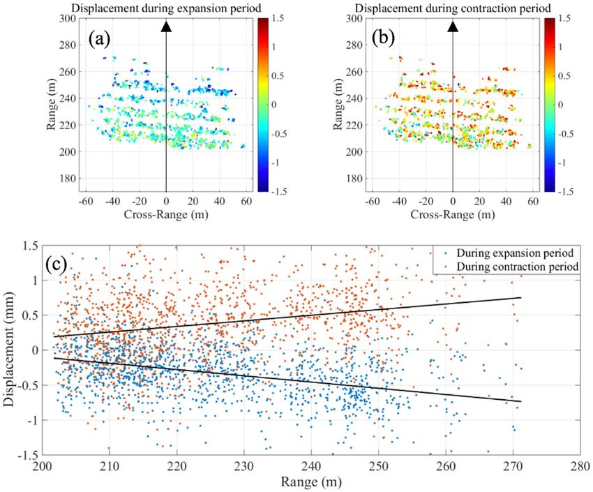
www.nature.com/scientificreports/
most pronounced near the surface, progressive damage can occur in large areas of the slopes. With time, this
generates a surficial layer of damaged material that is susceptible to instability. When a portion of this layer
fails, the falling debris tends to cause instability of the material downslope, and the scarp of the initiating failure
tends to destabilize material upslope. Therefore, shallow failures have the potential for large volume runouts.
Enhanced understanding of the fundamental mechanism of cyclic deformation in loess slopes can therefore lead
to improved monitoring strategies for landslide risk management in loess regions.
In this paper, we use the term “soil” in an engineering sense to refer to unconsolidated and poorly consolidated
surface and near-surface earth materials, including loess. Thermal shock occurs when temperature changes within
the soil mass are sufficiently large that the material cannot accommodate the resulting strains without suffering
damage. This damage represents a reduction in soil strength, as bond breakage reduces the cohesive component
of strength. Commonly, deformation caused by temperature changes is not large enough to cause significant
damage, however fatigue caused by the cyclic behavior progressively weakens the strength of the soil. In the long
term, this process can lead to degradation of the soil strength to a point of imminent f ailure8.
The effect of temperature-induced deformations has been previously studied, with examples of thermal cyclic
deformations and fatigue including the annual and daily displacements of tall engineered s tructures9, rock
slopes10, embankments11, as well as rock fall processes triggered by cyclic thermal stresses acting on exfoliation
fractures12. However, the authors are not aware of work attempting to quantify the relationship between thermal
fluctuation, deformations in loess slopes, and their effects on potential slope failures.
In order to gain insight into the relationship between weather and slope deformation, robust slope moni-
toring strategies are required to provide accurate, repeatable, and frequent information. Traditional geodetic
techniques for landslide monitoring include l eveling13 and GPS (Global Positioning System)14,15. Although these
techniques can provide highly accurate deformation measurements, the measurements are spatially sparse.
Spaceborne InSAR (synthetic aperture radar interferometry) techniques have been widely used in surface defor-
mation monitoring16–19 and provide land deformation maps in the line of sight between the satellite and the
area of interest. However, their sampling frequency depends on the satellite revisit period, which can range
between days and weeks depending on the satellite system used and the location of the area of interest. GB-SAR
(Ground-based Synthetic Aperture Radar) has been developed during the last d ecade20 and is characterized by
finer spatial resolution than satellite instruments (less than one meter compared to 3 m × 3 m at best for satellite
instruments), and high frequency of data acquisition (several images per hour)21. GB-SAR was adopted in this
study for monitoring the loess slope deformation patterns.
The temperature-dependent behavior raises the question of the potential impact of a changing climate in the
amount of strain imposed to loess slopes. During the twentieth century, Earth’s surface temperature increased
by approximately 0.6 °C, and additional warming is anticipated through the present c entury22. Discussion on
the impacts of global warming have focused on glacier and ice sheet melting, sea-level rise, and extreme weather
events, such as cyclones, floods, and droughts; and less so on the effects of local and regional increases in landslide
frequency, in particular the stability of loess slopes. Understanding the potential effects of climate change in the
stability of loess slopes becomes increasingly important for sustainable development in these areas.
In this paper, we present the spatial–temporal characteristics of the deformation of a loess slope and show how
the deformation correlates to moisture content and temperature fluctuation. The effects of changes in soil tem-
perature and moisture on the loess slope deformation are analyzed using both empirical and physical models. We
propose a mechanism that explains such behavior, validated with observations from high-frequency deformation
and weather data. The mechanism is used to develop a model to estimate short term effects of weather fluctua-
tions, and the impact of increasing temperatures due to climate change, on the short-term cyclic and long-term
average expansion of the slope. The loess slope that is the subject of this work was excavated on the side of a valley
slope and is approximately 70-m high (Fig. 1). The location is near the city of Yan’an, in Shanxi Province, China.
One year of slope surface displacements were measured using a GB-SAR unit and a displacement meter. Soil
temperature and moisture were also measured at the site (Fig. 2). The mechanisms and methods presented here
can be adopted at other loess-rich areas to better understand the potential impacts of a changing climate on the
deformation behavior of loess slopes and the increased potential for fatigue-induced damage and slope failure.
Study area and data acquisition
Study area. The study area is a loess slope near Yan’an, Shanxi Province, northwestern China (N 36°35′07″,
E 109°18′39″). Yanan is located in the central part of a loess plateau, with winters that are snowless and semi-dry.
Air moisture and temperature increase in the summers. The annual average temperature is 9.2 °C and the annual
average precipitation is 550 mm.
The loess slope of this study is a hillside cut excavated in 2015 to increase the available land for farming.
Measures to reinforce the slope, including planting vegetation and installing drainage channels, were completed
by early 2017. The slope geometry consists of six benches. The elevation at the bottom is 1190 m above sea level
(a.s.l.) and the slope length of 230 m. The elevation at the top of the slope is 1260 m a.s.l., and the slope length
there is 150 m. The total area of the slope is approximately 13,000 m2. The average slope angle is 48°. During the
monitoring campaign, the planted vegetation was still small and sparse, resulting in a relatively bare slope, ideal
for GB-SAR monitoring. A photograph of the test site is shown in Fig. 1.
Data acquisition. GB‑SAR system. The GB-SAR sensor used in this study is an Image by Interferomet-
ric Survey-L (IBIS-L) system made by Ingegneria Dei Sistemi (IDS). The sensor has a Ku band antenna with a
wavelength of approximately 1.72 cm and a maximum effective range of 4 km. It can provide line-of-sight (LOS)
deformation information with a precision of up to 0.1 mm under ideal c onditions23. The sensor was installed on
a stable solid horizontal base, approximately 200 m across the valley from the slope. During one year, from 30
Scientific Reports | (2021) 11:2250 | https://doi.org/10.1038/s41598-021-81821-4 2
Vol:.(1234567890)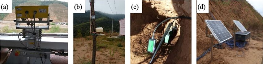
www.nature.com/scientificreports/

                                  Figure 1.  (a) Location of the loess slope and the distribution of loess and loess-like soils (green shading). (b)
                                  View of the loess slope near Yan’an. The red dots indicate the locations of instruments.

                                  Figure 2.  (a) GB-SAR instrument facing the slope. (b) Weather station for collecting meteorological data,
                                  installed on a pole approximately 2 m from the GB-SAR instrument and 1.5 m above the ground surface. (c)
                                  Hygrothermograph for collecting soil temperature and moisture data at four depths (0.1, 0.25, 0.4, and 0.6 m
                                  into the slope), installed at sites 1 and 2 (Fig. 1). The photo was taken prior to inserting the sensors into the
                                  slope. (d) Solar panels and the box containing the data acquisition system.

                                   Parameter                  Value      Parameter                  Value
                                   Maximum range              500 m      Antenna type               3 (Gain = 19) dBi)
                                   Center wavelength          17.4 mm    Scan length                2m
                                   Central frequency          17.2 GHz   Acquisition length         368 s
                                   Range resolution           0.8 m      Inter acquisition delay    532 s
                                   Azimuth angle resolution   4.4 mrad   Repeat observation cycle   900 s

                                  Table 1.  GB-SAR measurement parameters used for the campaign.

                                  September 2018 to 30 September 2019, a dataset of 24,518 images was acquired by the IBIS-L instrument. The
                                  measurement parameters used for the campaign are summarized in Table 1. A photograph of the field set-up of
                                  the IBIS-L system is shown in Fig. 2a.
                                     A weather station was installed on a pole approximately 2 m from the GB-SAR instrument and 200 m from
                                  the slope (Fig. 2). The weather station measured relative humidity, temperature, and pressure every 5 min.

Scientific Reports |   (2021) 11:2250 |                   https://doi.org/10.1038/s41598-021-81821-4                                                   3

                                                                                                                                                 Vol.:(0123456789)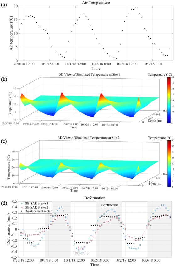
www.nature.com/scientificreports/
In‑situ measurements. To verify the results of the GB-SAR system, we installed a displacement meter vertically
in the bottom bench of the loess slope (Fig. 2). The measuring range and the accuracy of the displacement meter
are 25 mm and 0.02 mm, respectively. The buried depth is 2 m, where the displacement is assumed to be 0 mm.
Thus, measured displacement is relative to the position at that depth.
Eight hygrothermographs, which measure soil temperature and moisture, were placed at two sites (site 1 and
site 2) on the loess slope (Fig. 1). At each site, four hygrothermographs were placed at depths of 0.1 m, 0.25 m,
0.4 m and 0.6 m, respectively (Fig. 2c). A data acquisition system was placed on the bottom bench of the loess
slope to collect the data measured by these sensors (Fig. 2d). The data acquisition system consists of a solar power
supply system and data collectors. The data acquisition cycle is 5 min.
A digital elevation model (DEM) is required to interpret the deformation measured by the GB-SAR. The DEM
of the slope was generated through photogrammetry from images acquired with an unmanned aerial vehicle
(UAV). The original 0.1 m pixel resolution of the DEM was resampled to 0.5 m.
Methods
GB‑SAR interferometry. For continuous GB-SAR observations, the spatial baseline can be defined as 0 m.
Hence, unlike satellite SAR, there is no flat-earth phase. Ignoring thermal noise and other errors, the unwrapped
interferometric phase Δφ21 for images acquired at times 1 and 2 can be described by24–26:
�ϕ 21 = ϕ2 − ϕ1 = �ϕ 0 + �ϕ dis + �ϕ atm = �ϕ geom (1)
4πfc �r
�ϕ dis = (2)
c
where φ1 and φ2 are the phase of images acquired at time 1 and time 2, respectively. Δφ0 is a measure of the
change in the backscatter phase of targets, which can be ignored for persistent targets. Δφdis is linearly related
to displacement Δr along the line-of-sight direction deformation. Δφatm and Δφgeom are the errors introduced
by atmosphere changing and rail moving. We estimated these two errors and corrected for t hem21,27,28. The data
preprocessing was done using IBISDV (IBIS Data Viewer) software.
Heat conduction equation. The temperature of one-dimensional isotropic soil can be described by the
classical heat diffusion equation29, with the following solution30:
−
T(z, t) =T +T0 exp −z ω/2α sin wt − z ω/2α (3)
α = /c (4)
where T(z,t) is the temperature (°C) at time t (s) and depth z (m), and z is positive in the downward direction. α
is the apparent thermal diffusivity, c and λ are the volumetric heat capacity (J m-3 °C-1) and the apparent thermal
conductivity (W m-1 °C-1), respectively. c and λ may vary with time and depth; for a homogeneous case, they are
assumed to be independent of depth and time. The boundary conditions of Eq. (3) are as follows:
−
T(0, t) =T +T0 sin(wt) (5)
−
T(∞, t) =T (6)
T(z, 0) = f (z) (7)
where T (0,t) is the soil temperature at depth 0 m, and T (∞,t) is soil temperature when depth tends to infin-
ity. For simplicity, T (∞,t) is−defined as the soil temperature at the depth where the soil temperature does not
vary and remains steady at T . T (z,0) is the soil temperature at the initial time. f(z) can be a function of depth
or a known constant. T0 is the amplitude of the temperature sine function at the surface, ω = 2π/P is the radial
frequency, and P is the period of the fundamental cycle. From Eq. (3), the apparent thermal diffusivity α can be
expressed as f ollows31:
2
ω z2 − z1
α= (8)
2 ln(A1 /A2 )
2
1 z2 − z1
α= (9)
2ω t2 − t1
where A1 and A2 are the amplitude of the temperature sine function at depth z1 and z2 , respectively; and t1 and t2
are the time interval between measured occurrences of maximum soil temperature at depths z1 and z2 , respec-
tively. Accurate measurements of t1 and t2 are required. The amplitude decreases exponentially with depth, and
at a certain depth, it can be estimated by the daily maximum temperature Tmax and minimum temperature Tmin:
Scientific Reports | (2021) 11:2250 | https://doi.org/10.1038/s41598-021-81821-4 4
Vol:.(1234567890)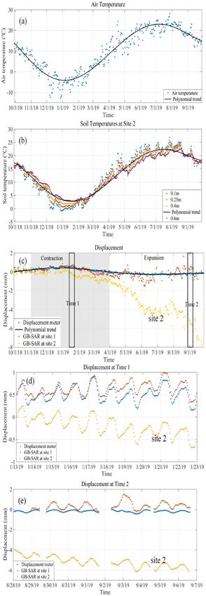
www.nature.com/scientificreports/
Tmax − Tmin
A= (10)
2
Additionally, the finite element difference method can be used to solve Eq. (3)32:
k k k
Ti,j+1 = α 2 Ti+1,j + 1 − 2α 2 Ti,j + α 2 Ti−1,j (11)
h h h
where Ti,j+1 is the soil temperature at the ith soil layer and (j + i)th time, k is the time interval, and h is the depth
interval. When α (k/h2) is less than 1/2, the differential scheme is stable and convergent, i.e. the result is reliable.
In this study, we measured soil temperatures at depths of 0.1 m, 0.25 m, 0.4 m, and 0.6 m with the hygro-
thermographs. In the daily soil temperature simulation, k and h are equal to 0.5 h and 0.05 m, respectively. The
apparent thermal diffusivity is assumed to be 1.98 × 10⁻³ m2 h−1. According to the soil temperature measurements
at the four depths, the daily soil temperature at depth− of 0.6 m under fair-weather conditions is stable, which can
be defined as the boundary condition (Eq. 6), i.e. T .
The soil temperature simulation is divided into two steps. The first step is to estimate the soil temperature at
depth of 0.05 m, which is the boundary condition in the second step (Eq. 5). Thus, soil temperatures are estimated
from a depth of 0.1 m to a depth of 0.6 m, and the soil temperatures at the depths of 0.1 m and 0.6 m are the
boundary conditions of Eqs. (5) and (6), respectively. The times of the maximum and minimum soil temperature
at a depth of 0.05 m are calculated from Eq. (9). The amplitude of the soil temperature at a depth of 0.05 m is −
calculated from Eqs. (8) and (10). The maximum soil temperature at a depth of 0.05 m is equal to the sum of T
and half of the amplitude of the soil temperature at 0.05 m depth. Similarly, the minimum soil temperature at
a depth of 0.05 m is equal to the difference between the two variables. With this procedure, the value and the
time of the maximum and the minimum soil temperatures at a depth of 0.05 m are calculated. The second step
estimates the soil temperature from a depth of 0.05 m to 0.6 m. The soil temperature at a depth 0.05 m and 0.6 m
are the boundary conditions of Eqs. (5) and 6. In the two steps, the boundary condition (Eq. 7) is simulated by
the soil temperature at depths 0 m, 0.1 m, 0.25 m, 0.4 m, and 0.6 m at the initial time.
Because the boundary condition (Eq. 7) is a very rough estimate, the preceding results of simulations are not
highly accurate and should be excluded. Thus, in daily soil temperature simulations, we exclude the preceding
one-day results. According to the measured soil moisture, we cannot assume that soil temperature at a depth of
2 m is constant throughout the year, and thus in the annual soil temperature simulation, the boundary condition
(Eq. 6) is not known. The annual soil temperature is not simulated by the heat conduction equation.
Calculation of heat energy related to thermal deformation. The heat energy exchange within one
hour of soil of a specific thickness can be divided into three terms: the energy exchange with the atmosphere
across the soil surface, the energy transferred from the previous time intervals, and the energy transferred to
the subsequent time intervals. It is assumed that within an hour, the second and third terms are equal at each
location. Therefore, the heat energy related to the change in soil temperature and the thermal deformation are
assumed equal to the first term, which can be expressed a s33:
n
w=
i=1
cvi Ti (12)
where w is the heat energy in J absorbed or released by the soil surface; Cvi and ΔTi are the volumetric heat capac-
−3 K−1) and the change of temperature of the ith layer of moist soil, respectively; and n is the number of
ity (J m
soil layers. In this study, the soil from 0 to 0.6 m was divided into 12 layers (i.e. n = 12). According to previous
research, the volumetric heat capacity Cv of the moist soil can be expressed by34,35:
Cv = Cw θ + Cs ρs (13)
where Cw is the volumetric heat capacity of water, assumed to be 4.20 × 10 J m K ; θ is the volumetric soil water
6 −3 −1
content; Cs is the volumetric heat capacity of dry soil; and ρs is the bulk density of the soil. We measured the volu-
metric soil water content at depths of 0.1, 0.25, 0.4, and 0.6 m with the hygrothermographs and derived θ from 0
to 0.6 m by linear interpolation. Here, we take Cs to be 0.8 × 10³ J kg−1 K−1 and estimate ρs to be 1.4 × 10³ kg m−3
for site 1 and 1.52 × 10n kg m−3 for site 2 based on laboratory measurements of samples collected at the site.
Thermal deformation model. In thermal deformation (expansion and contraction), the change in length
ΔL of a sample of loess material caused by a temperature change can be expressed by:
�L = β�TL (14)
where L (m) is the initial length of the sample at room temperature, ΔT (°C) is the change in temperature, and β
(°C−1) is the linear thermal expansion coefficient of the sample. In this paper, the temperature of the loess varies
with depth, therefore the expansion and contraction ΔL of the whole slope caused by the temperature change
can be derived as.
n
�L =
1
β�Ti Li (15)
where Li is the initial thickness of the ith loess layer, and ΔT is the change in temperature of the ith loess layer. β
is the linear thermal expansion coefficient of loess, and in this study, is independent of temperature. As only the
daily soil temperature is available from the heat conduction equation, we simulated the thermal deformation in
Scientific Reports | (2021) 11:2250 | https://doi.org/10.1038/s41598-021-81821-4 5
Vol.:(0123456789)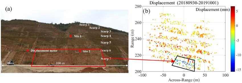
www.nature.com/scientificreports/
the daily deformation cycles. The loess soil from a depth of 0.1 m to a depth of 0.6 m is divided into 12 layers,
each 0.05 m thick. The linear expansion coefficient β of common materials is about 1 0–6 ~ 10–5 °C−136, The linear
thermal expansion coefficient of loess is approximately 35 × 10–5 °C−137,38.
Results and discussion
Observed slope deformation. Daily observations. We show daily observations of slope deformation
for a three-day period (30 September to 3 October 2019) in Fig. 3. Measured air temperature and simulated soil
temperature with depth are also shown in this figure. The simulated soil temperatures are derived from hydro-
thermograph measurements and heat conduction equations, as described above.
Air temperature cycles (Fig. 3a) show a minimum temperature near 1 °C, reached at about 7:00, and a maxi-
mum temperature near 17 °C, reached at about 15:00. The air heats up faster than it cools down at the study area.
Similarly, soil temperatures exhibit cyclic fluctuations, which is attributed to the changing solar radiation through
the day (Fig. 3b,c). Temperatures of the shallow soil are similar to air temperatures. The times of maximum and
the minimum soil temperatures increasingly lag air temperature extremes due to conduction of heat in the soil.
The amplitude of the soil temperature cycle decreases with depth, and at depths greater than 0.5 m there are no
measurable changes in soil temperature.
Deformation measured by the GB-SAR sensor is consistent with that recorded by the displacement meter
(Fig. 3d) and validates the cyclic patterns described above. The deformation measured by the GB-SAR sensor
shows a distinct, somewhat smooth sinusoidal pattern. The displacement meter data show an episodic contraction
and expansion. The overall pattern of the two sets of deformation measurement is similar, and the differences
between them are generally less than 0.1 mm. The GB-SAR deformation data are assumed to be representative
of the slope behavior and adopted for further analysis.
Maximum contraction generally happened between approximately 3:00 and 8:00, and the maximum expan-
sion occurred between 14:00 and 17:30. Between the times of maximum expansion and contraction, the surface
“breathing” is relatively continuous. The expansion period is defined as the interval when the surface expands
relative to the average position, typically between 10:30 and 22:30 (the white background in Fig. 3d). The con-
traction period is the interval when the surface contracts relative to the average position, typically from 22:30 to
10:30 (the gray background in Fig. 3d). Deformation measured by GB-SAR and soil temperatures appear highly
correlated, showing that soil expansion and contraction mainly follow the cyclic fluctuations of soil temperature
between 0 m (surface) and approximately 0.5 m depth into the slope.
Figure 3d shows that the maximum contraction and expansion at site 1 are larger than those at site 2. The
differences between the two sites stem from the fact that the soil temperature fluctuations at site 1 are larger
than those at site 2. Figure 4 shows the average soil temperatures as a function of depth at the two sites over
the same three days as in Fig. 3. It is clear from the data that the temperature changes at depths less than about
0.3 m are larger at site 1 than site 2. The maximum difference between the two sites is > 5 °C at a depth of 0 m,
decreasing to approximately 0 °C at depths > 0.3 m. We attribute these differences to differences in soil moisture
at the two sites.
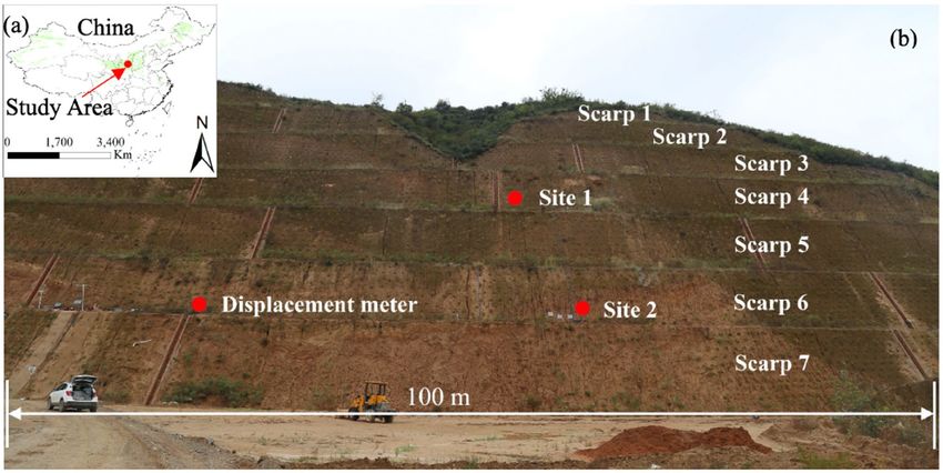
Spatially, the amplitudes of the difference between cyclic expansion and contraction increase linearly from
the bottom of the slope to the top (Fig. 5). To describe this spatial variation, Fig. 5 shows the surface deforma-
tion at the times of maximum expansion (16:14 on 30 September 2018) and maximum contraction (07:29 on 3
October 2018). The information is presented as a map of surface deformation from the perspective of the radar,
where range is the distance from the GB-SAR (lower range corresponds to the toe of the slope, higher range
corresponds to the crest) and cross-range is in the direction of the width of the slope, zeroed at the location of
the radar, and plotted against range (Fig. 5c). The graphs in Fig. 5 are in GB-SAR coordinates, with the location
of the GB-SAR sensor defined as the origin. The direction of the GB-SAR linear rail is the cross-range direction.
The direction perpendicular to the rail and along line-of-sight direction is defined as the range direction. At the
bottom of the slope (range in Fig. 5a,b = 201 m), the expansion and the contraction each average about 0.15 mm.
At the top of the slope (range 270 m in Fig. 5a,b), the expansion and the contraction average approximately
0.7 mm. The measured expansion has the same magnitude of the contraction, suggesting that the deformation
is recovered and in the elastic regime.
Annual observations. The annual cycles of daily average air and soil temperatures and slope expansion/contrac-
tion between 30 September 2018 and 1 October 2019 are shown in Fig. 6. Soil temperature differences between
the two sites are not significant compared to their fluctuations throughout the year, thus we only show data from
site 2 in Fig. 6b. The minimum air temperature at the study site, about − 5 °C, occurs in mid to late January; the
maximum of 23 °C is in late July to early August (Fig. 6b). As in the case of the annual cycles, the times of the
maximum and the minimum soil temperatures show a lag that increases with soil depth. Maximum and mini-
mum soil temperatures also decrease with depth, showing less variability as depth increases.
The annual cyclic contraction and expansion at site 1shows that deformations are recoverable, therefore
suggesting that no damage has occurred to the loess material and that the material strength is preserved. The
maximum contraction occurs approximately in mid to late January, and maximum expansion in late July and
early August. The amplitude of the average annual fluctuation is about 1 mm. The contraction period typically
extends from mid-November to mid-April of the following year (gray background in Fig. 9), and the expansion
period is from mid-April to mid-November (the white background in Fig. 9).
The annual cyclic deformation at site 2 shows that deformation towards the GB-SAR (out of slope) is not fully
recovered (Fig. 6c). The unrecovered cumulative deformation increases through the period. Figure 6d,e show the
same pattern –the daily cycles at site 2 have expansions that are not recovered during the contraction period, both
in cold and warm weather. This suggests that damage has occurred and that the material strength has been reduced.
Scientific Reports | (2021) 11:2250 | https://doi.org/10.1038/s41598-021-81821-4 6
Vol:.(1234567890)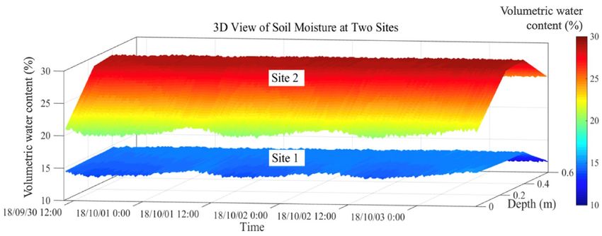
www.nature.com/scientificreports/
Figure 3. The daily cycle of temperature and deformation over three days from 10:15 on 30 September to 10:14
on 3 October 2018. (a) Air temperature. (b) and (c) 3D view of soil temperature at sites 1 and 2. (d) Comparison
of deformation measured by the GB-SAR sensor and the displacement meter. Negative and positive values
indicate deformation toward and away from the GB-SAR sensor, respectively. Temperature and deformation
fluctuation appear to be highly correlated. Air temperature and deformation were sampled every hour.
Figure 7 shows the deformation between 30 September 2018 and 1 October 2019. The red rectangle in Fig. 7a
and the black rectangle in Fig. 7b rectangle indicate the area of the slope where measured deformations were
not fully recovered, with approximately 8 to14 mm of out-of-slope deformation in one year, sufficient to cause
small-scale landslides39.
Scientific Reports | (2021) 11:2250 | https://doi.org/10.1038/s41598-021-81821-4 7
Vol.:(0123456789)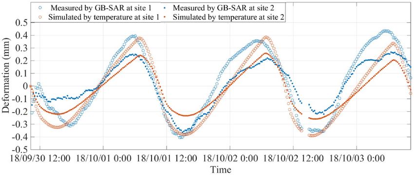
www.nature.com/scientificreports/

                                            Figure 4.  Average soil temperature from 0 to 0.6 m depth at sites 1 and 2 over a three-day period.

                                            Figure 5.  Slope displacements measured by the GB-SAR during (a) the maximum expansion period (16:14 on
                                            30 September 2018), and (b) the maximum contraction period (07:29 on 3 October 2018). (a) and (b) show the
                                            displacement maps, where range is the distance from the GB-SAR (lower range corresponds to the toe of the
                                            slope, higher range corresponds to the crest, and cross-range is in the direction of the width of the slope, zeroed
                                            at the location of the radar). (c) Displacement plotted against range with dark lines showing trends during the
                                            expansion/contraction periods, i.e. increasing cyclic displacements near the crest compared to the toe of the
                                            slope.

          Scientific Reports |   (2021) 11:2250 |                https://doi.org/10.1038/s41598-021-81821-4                                                   8

Vol:.(1234567890)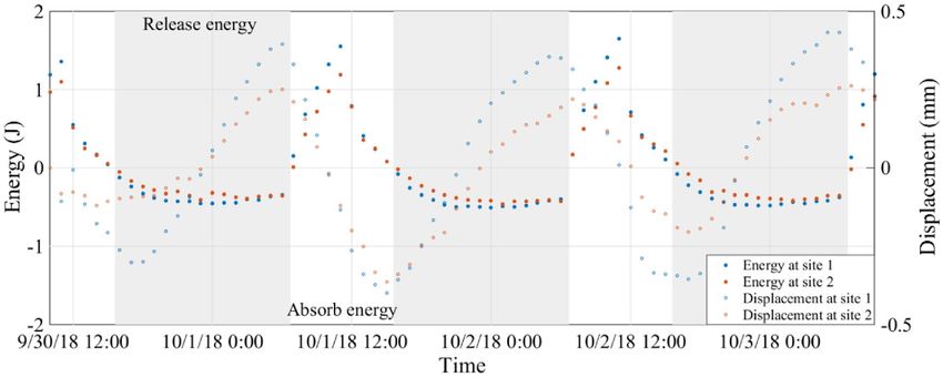
www.nature.com/scientificreports/

                                  Figure 6.  The annual cycle of air and loess temperature, and slope expansion/contraction between 30 September 2018 and
                                  1 October 2019. (a) Daily average air temperatures (dots) and their polynomial trend (black line). (b) Daily average soil
                                  temperatures (dots) at site 2 and their polynomial trend (black line) at four depths. (c) Daily deformation measured at sites
                                  1 and 2 with GB-SAR sensor and the displacement meter (black line is the polynomial trend for the displacement meter).
                                  (d) and (e) Deformation measured by the displacement meter and GB-SAR sensor between the 13 and 23 January 2019 and
                                  between August 28 and 17 September 2019. Negative and positive displacement values indicate movement towards and away
                                  from the GB-SAR sensor. Observations suggest a close correlation between air temperature and slope expansion/contraction
                                  at the annual scale.

Scientific Reports |   (2021) 11:2250 |                  https://doi.org/10.1038/s41598-021-81821-4                                                               9

                                                                                                                                                         Vol.:(0123456789)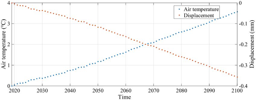
www.nature.com/scientificreports/

                                            Figure 7.  Slope deformation between 30 September 2018 and 1 October 2019. The red (a) and black
                                            (b) rectangles indicate the area showing non-recoverable deformation. Negative values are out-of-slope
                                            deformation.

                                            Figure 8.  3D view of soil volumetric water content from 0 to 0.6 m depth at sites 1 and 2 over a three-day
                                            period. Soil moisture contents at depths of 0.1, 0.25, 0.4, and 0.6 m were measured with hygrothermographs;
                                            values at other depths were calculated by linear interpolation.

                                            Figure 9.  Energy fluctuation at the two sites during a three-day interval, estimated from soil temperature and
                                            moisture data. Positive values indicate energy absorption (white background), and negative values indicate
                                            energy release (gray background).

          Scientific Reports |   (2021) 11:2250 |               https://doi.org/10.1038/s41598-021-81821-4                                                    10

Vol:.(1234567890)
www.nature.com/scientificreports/
Soil moisture. The soil volumetric water content at site 2 is consistently greater than that site 1 (11–15% at
site 1, and 20–30% at site 2) (Fig. 8). Rainfall infiltration is the major source of soil moisture at the study site.
Low infiltration due to the high slope angle (approximately 48°) and consequent high surface runoff result in
relatively low soil moisture at the top of the slope. Moisture is also lost at the top of the slope due to exposure
to wind. Rainwater infiltrates the lower part of the slope and ground water collects there, leading to higher soil
moisture40–42.
Despite these differences, soil moisture at the two sites has some similarities. The soil moisture at both sites
initially increases with depth and then decreases (Fig. 8). Water contents at both sites show the same diurnal
fluctuations, which are mainly the result of evapotranspiration. Soil moisture begins to decline at approximately
8:00 as the sun rises and evapotranspiration increases. In the late afternoon, around 16:30, evaporation decreases
as the slope is initially shadowed and the sun then sets, resulting in a small increase in soil moisture.
Mechanism of cyclic deformation of the loess slope. We propose that the observed correspondence
between temperature fluctuation and slope cyclic deformation reflects the response of the soil mass to tempera-
ture fluctuations at shallow depths, i.e. expansion and contraction of the loess grains. The amount of expansion
and contraction depends on the soil temperature variations caused by fluctuations in air temperature, the ther-
mal characteristics of loess grains, and the soil moisture content. This relationship can be quantified in terms of
heat energy and energy transfers between the air and the soil, and through the soil mass.
The heat energy at the two sites was calculated based on soil temperatures and moisture contents, and is
shown in Fig. 9. As expected, the energy has a cyclic daily fluctuation, which corresponds to energy transfers
between the soil and the air. As the sun rises (at 6:40 during the three-day interval), solar radiation begins to
increase and air temperature increases, soon becoming higher than that of the soil surface. At about 7:00, energy
begins to transfer from the atmosphere to the soil surface, the soil absorbs energy, and the energy flux turns
positive. At this moment, the soil temperature begins to increase, the amplitudes of atomic vibration in the soil
increase, and the average separation of the atoms increases, leading to volumetric change of the water and soil
grains. As a result, the loess deforms out of s lope43. In the afternoon, as the sun lowers toward the horizon, solar
radiation begins to decrease, and at approximately 15:00, the temperature of the air decreases and approaches
equilibrium with the soil surface. As air temperature continues to decrease, energy begins to transfer from the
soil surface towards the atmosphere, the soil releases energy, and the energy flux becomes negative. From the
time of maximum contraction to maximum expansion, the slope absorbs energy, and from the time of maximum
expansion to maximum contraction, the slope releases energy. In a daily cycle, the total values of absorbed and
released energy are generally equal; therefore energy is generally conserved during the daily “breathing” of the
slope except for minor temperature differences from day to day.
We observed that the absolute calculated value of the energy at site 1 is sometimes larger (up to 19%) than that
at site 2. This difference possibly results from two factors. First, there is a difference in solar radiation at the two
sites, where direct sunlight reaches the crest of the slope sooner than the toe. This difference was observed in the
temperature fluctuation and changes with depth at the two sites. Second, soil moisture content is also different at
the two sites, therefore yielding a different energy transfer. Differences in soil temperature between sites are likely
controlled by differences in heat capacity, which in turn are mainly controlled by differences in soil moisture.
The amplitude of soil temperature change increases as the soil moisture decreases. Specifically, because soil
moisture at site 2 is higher than that of site 1, soil temperature changes at site 2 are lower than at site 1. The spatial
variation of soil moisture in the slope would have a substantial effect on the amount of energy transferred and
therefore will have a marked influence in the spatial variation of soil temperature and its manifestation in cyclic
deformation. Soil moisture at site 2 is higher than that of site 1, leading to a higher heat capacity at the former
site than the latter. Consequently, soil temperature fluctuations at site 1 are larger than those at site 2.
In our study, the hygrothermographs were installed at four depths (0.1, 0.25, 0.4, and 0.6 m), thus soil mois-
ture at depths > 0.6 m is unknown. Accordingly, a linear interpolation of soil moisture from 0.6 m to 2 m would
not be reliable. Therefore, we have not attempted to quantify energy changes on an annual basis. However, it is
understood that daily and annual cyclic deformations follow the same mechanism, therefore the slope absorbs
energy from the time of maximum contraction to maximum expansion and releases energy and from the time
of maximum expansion to the maximum contraction within each annual cycle.
Forecasting annual and daily deformation cycles, and what to expect with climate change. The
close relation between temperature fluctuations and the slope deformation cycle allows us to postulate a predic-
tive deformation model for the loess slope. The daily deformation cycles measured by GB-SAR and simulated
by temperature at the two sites between 30 September and 3 October 2019 are shown in Fig. 10. The agreement
between the measured and simulated daily deformation cycle supports the postulated mechanism and the inf-
dataluence of moisture and soil temperature at depths up to 0.6 m. However, we do not have soil temperature
throughout the year and thus cannot simulate the soil temperature and thermal deformation in annual cycles.
The predictive model also provides a tool to explore the potential effects of climate change on the cyclic defor-
mation of the loess slope. Temperature extremes are difficult to predict, but a first approximation of the effect of
warmer climate on the loess slope can be made by considering the maximum amplitude of slope deformation
observed in the present-day daily cycles (about 1 mm) to that expected for average temperatures in the future.
By the end of this century, assuming the IPCC high-emission scenario RCP (representative concentration path-
way) 8.5, the global average temperature will be 3.5 °C higher than today44. Given that energy rapidly transfers
between the atmosphere and the soil, we assume the surface soil temperature, on average, will increase by the
same amount. The heat conduction equation can be used to calculate future soil temperatures with depth in
the loess slope in that we have studied, assuming a linear increase in average air temperature increase of 3.5 °C
Scientific Reports | (2021) 11:2250 | https://doi.org/10.1038/s41598-021-81821-4 11
Vol.:(0123456789)www.nature.com/scientificreports/
Figure 10. Deformation measured by the GB-SAR sensor at sites 1 and 2, and simulated deformation based on
thermal deformation model and temperature measurements.
Figure 11. Projected air temperature and deformation of the loess slope on 15 January of each year from 2020
to 2100, referenced to 2020. Negative values indicate deformation toward the GB-SAR sensor (expansion of the
slope). The loess slope expands to 0.35 mm (average, without considering annual and daily breathing cycles) as
atmosphere temperature increases 3.5 °C.
between now and 2020. Figure 11 shows temperature and deformation for the time on January 15 of every year
from 2020 to 2100 when the air temperature is at a minimum and the contraction of the slope is at a maximum
in the annual cycle. Because we are calculating the relative increase in average slope expansion due to the average
increase in temperature, the choice of the time of year does not affect the calculations and conclusions. Figure 11
shows that with an assumed increase in air temperature of 3.5 °C from 2020 to 2100, the loess slope will expand
an average of 0.35 mm. This represents a 70% increase in expansion during the daily cycle in comparison to the
present deformation. As the air temperature increases, the increasing transfer of energy from the atmosphere to
the soil will lead to a substantial increase in deformation, which will contribute to an accelerated thermal fatigue
of the loess forming the slope. This could lead to accelerated deterioration of the shallow layers of the loess slope
and failure due to gravitational forces.
Conclusions
We have documented the spatio-temporal characteristics of cyclic expansion and contraction of a loess slope near
Yan’an, in Shanxi Province, northwestern China using GB-SAR technology. The mechanism of deformation was
analyzed using empirical and physical models of soil temperature and moisture. Our conclusions are as follows:
(1) The loess slope shows daily and annual cyclic expansion and contraction, which mainly result from the
cyclic fluctuation of soil temperature.
(2) The cyclic expansion and contraction are caused by energy transfers. When the slope moves outward, it
absorbs energy, and when the slope moves inward, it releases energy. This is reflected in volumetric changes of
the water within the soil and differences in excitation of the soil particles.
(3) Soil volume changes are associated with stress changes in the soil. Fully recovered deformations between
cycles suggest that deformations are within the elastic regime of the loess material. Non-recoverable deforma-
tions, observed at one site on an annual timescale, suggest damage of the loess (breakage of bonds between soil
grains) and therefore a loss in soil strength.
Scientific Reports | (2021) 11:2250 | https://doi.org/10.1038/s41598-021-81821-4 12
Vol:.(1234567890)www.nature.com/scientificreports/
(4) Cyclic expansion and contraction characteristics of a loess slope can be used to evaluate damage in the
soil materials that could lead to surficial slope failures.
(5) Increases in temperature predicted by some climate change models suggest that cyclic deformations of
the loess slope at our study site might increase by approximately 70%.
Received: 9 October 2020; Accepted: 11 January 2021
References
1. Lin, N.-F. & Tang, J. Geological environment and causes for desertification in arid-semiarid regions in China. Environ. Geol. 41(7),
806–815 (2002).
2. Lin, Z. & Liang, W. Engineering properties and zoning of loess and loess-like soils in China. Can. Geotech. J. 19(1), 76–91 (1982).
3. Xinbao, Z., Higgitt, D. L. & Walling, D. E. A preliminary assessment of the potential for using caesium-137 to estimate rates of soil
erosion in the Loess Plateau of China. Int. Assoc. Sci. Hydrol. Bull. 35(3), 243–252 (1991).
4. Orden, D., Gao, L., Xue, X., Peterson, E. & Thornsbury, S. Technical Barriers Affecting Agricultural Exports from China: The Case
of Fresh apples. Draft Report (International Food Policy Research Institute, Washington, D.C., 2007).
5. Jiang, J.-P. et al. Soil microbial activity during secondary vegetation succession in semiarid abandoned lands of Loess Plateau.
Pedosphere 19(6), 735–747 (2009).
6. Hall, K. The role of thermal stress fatigue in the breakdown of rock in cold regions. Geomorphology 31(1–4), 47–63 (1999).
7. Hœrlé, S. Rock temperatures as an indicator of weathering processes affecting rock art. Earth Surf. Proc. Land. 31(3), 383–389
(2006).
8. Mufundirwa, A. et al. Analysis of natural rock slope deformations under temperature variation: A case from a cool temperate
region in Japan. Cold Reg. Sci. Technol. 65(3), 488–500 (2011).
9. Xia, Y. et al. Deformation monitoring of a super-tall structure using real-time strain data. Eng. Struct. 67, 29–38 (2014).
10. Gunzburger, Y., Merrien-Soukatchoff, V. & Guglielmi, Y. Influence of daily surface temperature fluctuations on rock slope stability:
case study of the Rochers de Valabres slope (France). Int. J. Rock Mech. Min. Sci. 42(3), 331–349 (2005).
11. Ma, W. et al. Characteristics and mechanisms of embankment deformation along the Qinghai-Tibet Railway in permafrost regions.
Cold Reg. Sci. Technol. 67(3), 178–186 (2011).
12. Collins, B. D. & Stock, G. M. Rockfall triggering by cyclic thermal stressing of exfoliation fractures. Nat. Geosci. 9(5), 395 (2016).
13. Gikas, V. & Sakellariou, M. Settlement analysis of the Mornos earth dam (Greece): Evidence from numerical modeling and geodetic
monitoring. Eng. Struct. 30(11), 3074–3081 (2008).
14. Nilforoushan, F. et al. GPS network monitors the Arabia-Eurasia collision deformation in Iran. J. Geodesy 77(7–8), 411–422 (2003).
15. He, X. et al. Application and evaluation of a GPS multi-antenna system for dam deformation monitoring. Earth Planets Space
56(11), 1035–1039 (2004).
16. Meng, Y. et al. Characteristics of surface deformation detected by X-band SAR interferometry over Sichuan-Tibet grid connection
project area. China. Remote Sens. 7(9), 12265–12281 (2015).
17. Lan, H. Complex urban infrastructure deformation monitoring using high resolution PSI. IEEE J. Sel. Top. Appl. Earth Obs. Remote
Sens. 5(2), 643–651 (2012).
18. Lan, H. et al. Integration of TerraSAR-X and PALSAR PSI for detecting ground deformation. Int. J. Remote Sens. 34(15), 5393–5408
(2013).
19. Xuguo, S. et al. Mapping and characterizing displacements of active loess slopes along the upstream Yellow River with multi-
temporal InSAR datasets. Sci. Total Environ. 674, 200–210 (2019).
20. Pipia, L. et al. A comparison of different techniques for atmospheric artefact compensation in GBSAR differential acquisitions.
In IGARSS 2006: IEEE International Geoscience and Remote Sensing Symposium, 31 July–4 August 2006, Denver, Colorado (IEEE,
2006).
21. Zhao, X. et al. A multiple-regression model considering deformation information for atmospheric phase screen compensation in
ground-based SAR. IEEE Trans. Geosci. Remote Sens. 99, 1–13 (2019).
22. Houghton, J. et al. Climate Change 2001: The Science of Climate Change. Contribution of Working Group I to the Intergovernmental
Panel on Climate Change Third Assessment Report (Cambridge University Press, New York, 2001).
23. Luzi, G., Crosetto, M. & Monserrat, O. Advanced techniques for dam monitoring. In Proceedings of the 2nd International Congress
on Dam Maintenance and Rehabilitation, Zaragoza, Spain (2010).
24. Noferini, L. et al. Long term landslide monitoring by ground-based synthetic aperture radar interferometer. Int. J. Remote Sens.
27(10), 1893–1905 (2006).
25. Pieraccini, M. et al. Ground-based SAR for short and long term monitoring of unstable slopes. In 2006 European Radar Conference.
(IEEE, 2006).
26. Rödelsperger, S. et al. Monitoring of displacements with ground-based microwave interferometry: IBIS-S and IBIS-L. J. Appl.
Geodesy 4(1), 41–54 (2010).
27. Iglesias, R. et al. Atmospheric phase screen compensation in ground-based SAR with a multiple-regression model over mountain-
ous regions. IEEE Trans. Geosci. Remote Sens. 52(5), 2436–2449 (2014).
28. Yang, H. et al. A correcting method about GB-SAR rail displacement. Int. J. Remote Sens. 38(5–6), 1483–1493 (2017).
29. Hanks, R., Austin, D. & Ondrechen, W. T. Soil temperature estimation by a numerical method. Soil Sci. Soc. Am. J. 35(5), 665–667
(1971).
30. Jackson, R. D. & Kirkham, D. Method of measurement of the real thermal diffusivity of moist soil. Soil Sci. Soc. Am. J. 22(6),
479–482 (1958).
31. Horton, R., Wierenga, P. & Nielsen, D. Evaluation of methods for determining the apparent thermal diffusivity of soil near the
surface. Soil Sci. Soc. Am. J. 47(1), 25–32 (1983).
32. Zhang, D. et al. Laboratory experimental study of infrared imaging technology detecting the conservation effect of ancient earthen
sites (Jiaohe Ruins) in China. Eng. Geol. 125, 66–73 (2012).
33. Dane, J. H. & Topp, C. G. Methods of Soil Analysis, Part 4: Physical Methods (Wiley, New York, 2020).
34. Alnefaie, K. A. & Abu-Hamdeh, N. H. Specific heat and volumetric heat capacity of some saudian soils as affected by moisture and
density. In International Conference on Mechanics, Fluids, Heat, Elasticity and Electromagnetic Fields (2013).
35. Cass, A., Campbell, G. & Jones, T. Enhancement of thermal water vapor diffusion in soil 1. Soil Sci. Soc. Am. J. 48(1), 25–32 (1984).
36. Plueddemann, E. P. Nature of adhesion through silane coupling agents. In Silane Coupling Agents (ed. Plueddemann, E. P.) 111–139
(Springer, Berlin, 1982).
37. McTigue, D. Thermoelastic response of fluid-saturated porous rock. J. Geophys. Res. 91(B9), 9533–9542 (1986).
38. Mordovskii, S., Vychuzhin, T. & Petrov, E. Coefficients of linear expansion of freezing soils. J. Min. Sci. 29(1), 39–42 (1993).
39. Li, L., Lan, H. & Peng, J. Loess erosion patterns on a cut-slope revealed by LiDAR scanning. Eng. Geol. 268, 105516 (2020).
40. Ramos, M. & Martínez-Casasnovas, J. Impact of land levelling on soil moisture and runoff variability in vineyards under different
rainfall distributions in a Mediterranean climate and its influence on crop productivity. J. Hydrol. 321(1–4), 131–146 (2006).
Scientific Reports | (2021) 11:2250 | https://doi.org/10.1038/s41598-021-81821-4 13
Vol.:(0123456789)www.nature.com/scientificreports/
41. Minet, J. et al. Mapping shallow soil moisture profiles at the field scale using full-waveform inversion of ground penetrating radar
data. Geoderma 161(3–4), 225–237 (2011).
42. Tabor, J. A. Improving crop yields in the Sahel by means of water-harvesting. J. Arid Environ. 30(1), 83–106 (1995).
43. White, G. Solids: Thermal expansion and contraction. Contemp. Phys. 34(4), 193–204 (1993).
44. Stocker, T. F. et al. Climate Change 2013: The Physical Science Basis. Contribution of Working Group I to the Fifth Assessment Report
of IPCC the Intergovernmental Panel on Climate Change (Cambridge University Press, New York, 2014).
Acknowledgements
Our research was supported by the National Natural Science Foundation of China (Grant Nos. 41790443,
41927806, 41941019, and 41421001), the National Key R&D Program of China (Grant No. 2019YFC1520601),
the Second Tibetan Plateau Scientific Expedition and Research (STEP) program (Grant No. 2019QZKK0904),
the Strategic Priority Research Program of Chinese Academy of Sciences (CAS) (Grant Nos. XDA23090301 and
XDA19040304), and the Key Research Program of Frontier Sciences of Chinese Academy of Sciences (CAS)
(Grant No. QYZDY-SSW-DQC019).
Author contributions
H.L.: Design of the experiment, review of results, data interpretation and drafting of the manuscript. X.Z.: data
acquisition and interpretation, review of manuscript. R.M.: Design of experiments, data interpretation, review of
results, manuscript drafting. J.P.: data acquisition, data processing. L.L.: Design of experiments, data acquisition,
data processing and interpretation. Y.W.: data processing and interpretation. X.L.: design of experiments, data
acquisition and interpretation. N.Z.: data acquisition and processing. S.L.: design of experiment, data acquisition
and interpretation. C.Z.: design of experiment, data processing, drafting of manuscript. J.C.: design of experi-
ments, data interpretation, drafting of manuscript. Y.Z.: data interpretation, drafting of manuscript.
Competing interests
The authors declare no competing interests.
Additional information
Correspondence and requests for materials should be addressed to H.L. or R.M.
Reprints and permissions information is available at www.nature.com/reprints.
Publisher’s note Springer Nature remains neutral with regard to jurisdictional claims in published maps and
institutional affiliations.
Open Access This article is licensed under a Creative Commons Attribution 4.0 International
License, which permits use, sharing, adaptation, distribution and reproduction in any medium or
format, as long as you give appropriate credit to the original author(s) and the source, provide a link to the
Creative Commons licence, and indicate if changes were made. The images or other third party material in this
article are included in the article’s Creative Commons licence, unless indicated otherwise in a credit line to the
material. If material is not included in the article’s Creative Commons licence and your intended use is not
permitted by statutory regulation or exceeds the permitted use, you will need to obtain permission directly from
the copyright holder. To view a copy of this licence, visit http://creativecommons.org/licenses/by/4.0/.
© The Author(s) 2021
Scientific Reports | (2021) 11:2250 | https://doi.org/10.1038/s41598-021-81821-4 14
Vol:.(1234567890)You can also read