ActiveStereoNet: End-to-End Self-Supervised Learning for Active Stereo Systems - CVF Open Access
←
→
Page content transcription
If your browser does not render page correctly, please read the page content below
ActiveStereoNet: End-to-End Self-Supervised
         Learning for Active Stereo Systems

    Yinda Zhang1,2 , Sameh Khamis1 , Christoph Rhemann1 , Julien Valentin1 ,
         Adarsh Kowdle1 , Vladimir Tankovich1 , Michael Schoenberg1 ,
            Shahram Izadi1 , Thomas Funkhouser1,2 , Sean Fanello1
                         1
                             Google Inc., 2 Princeton University

       Abstract. In this paper we present ActiveStereoNet, the first deep
       learning solution for active stereo systems. Due to the lack of ground
       truth, our method is fully self-supervised, yet it produces precise depth
       with a subpixel precision of 1/30th of a pixel; it does not suffer from the
       common over-smoothing issues; it preserves the edges; and it explicitly
       handles occlusions. We introduce a novel reconstruction loss that is more
       robust to noise and texture-less patches, and is invariant to illumination
       changes. The proposed loss is optimized using a window-based cost ag-
       gregation with an adaptive support weight scheme. This cost aggregation
       is edge-preserving and smooths the loss function, which is key to allow
       the network to reach compelling results. Finally we show how the task
       of predicting invalid regions, such as occlusions, can be trained end-to-
       end without ground-truth. This component is crucial to reduce blur and
       particularly improves predictions along depth discontinuities. Extensive
       quantitatively and qualitatively evaluations on real and synthetic data
       demonstrate state of the art results in many challenging scenes.

       Keywords: Active Stereo, Depth Estimation, Self-supervised Learning,
       Neural Network, Occlusion Handling, Deep Learning

1    Introduction

Depth sensors are revolutionizing computer vision by providing additional 3D
information for many hard problems, such as non-rigid reconstruction [9, 8], ac-
tion recognition [10, 15] and parametric tracking [47, 48] . Although there are
many types of depth sensor technologies, they all have significant limitations.
Time of flight systems suffer from motion artifacts and multi-path interference
[5, 4, 39]. Structured light is vulnerable to ambient illumination and multi-device
interference [14, 12]. Passive stereo struggles in texture-less regions, where ex-
pensive global optimization techniques are required - especially in traditional
non-learning based methods.
     Active stereo offers a potential solution: an infrared stereo camera pair is
used, with a pseudorandom pattern projectively texturing the scene via a pat-
terned IR light source. (Fig. 1). With a proper selection of sensing wavelength,
the camera pair captures a combination of active illumination and passive light,
2       Y. Zhang et al.

Fig. 1. ActiveStereoNet (ASN) produces smooth, detailed, quantization free results
using a pair of rectified IR images acquired with an Intel Realsense D435 camera. In
particular, notice how the jacket is almost indiscernible using the sensor output, and
in contrast, how it is clearly observable in our results.

improving quality above that of structured light while providing a robust solution
in both indoor and outdoor scenarios. Although this technology was introduced
decades ago [41], it has only recently become available in commercial products
(e.g., Intel R200 and D400 family [2]). As a result, there is relatively little prior
work targeted specifically at inferring depths from active stereo images, and large
scale training data with ground truth is not available yet.
    Several challenges must be addressed in an active stereo system. Some are
common to all stereo problems – for example, it must avoid matching occluded
pixels, which causes oversmoothing, edge fattening, and/or flying pixels near con-
tour edges. However, other problems are specific to active stereo – for example, it
must process very high-resolution images to match the high-frequency patterns
produced by the projector; it must avoid the many local minima arising from
alternative alignments of these high frequency patterns; and it must compensate
for luminance differences between projected patterns on nearby and distant sur-
faces. Additionally, of course, it cannot be trained with supervision from a large
active stereo dataset with ground truth depths, since none is available.
    This paper proposes the first end-to-end deep learning approach for ac-
tive stereo that is trained fully self-supervised. It extends recent work on self-
supervised passive stereo [58] to address problems encountered in active stereo.
First, we propose a new reconstruction loss based on local contrast normalization
(LCN) that removes low frequency components from passive IR and re-calibrates
the strength of the active pattern locally to account for fading of active stereo
patterns with distance. Second, we propose a window-based loss aggregation
with adaptive weights for each pixel to increase its discriminability and reduce
the effect of local minima in the stereo cost function. Finally, we detect occluded
pixels in the images and omit them from loss computations. These new aspects
of the algorithm provide significant benefits to the convergence during training
and improve depth accuracy at test time. Extensive experiments demonstrate
that our network trained with these insights outperforms previous work on active
stereo and alternatives in ablation studies across a wide range of experiments.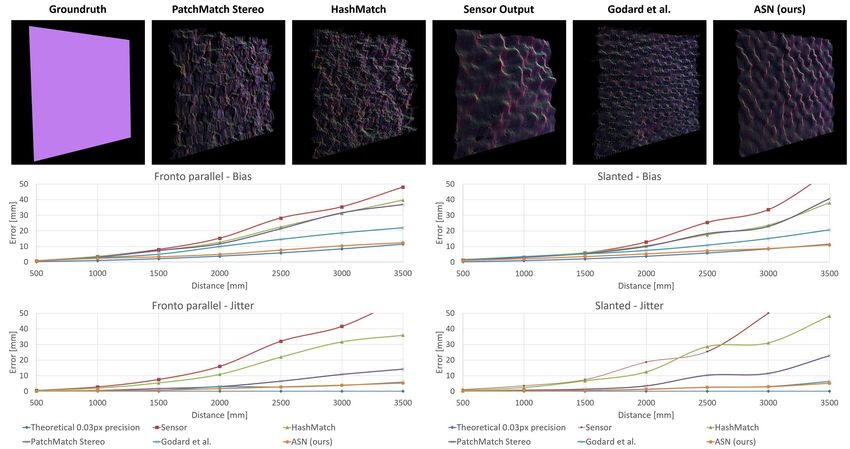
ActiveStereoNet        3

2    Related Work
Depth sensing is a classic problem with a long history of prior work. Among the
active sensors, Time of Flight (TOF), such as Kinect V2, emits a modulated
light source and uses multiple observations of the same scene (usually 3-9) to
predict a single depth map. The main issues with this technology are artifacts due
to motion and multipath interference [5, 4, 39]. Structure light (SL) is a viable
alternative, but it requires a known projected pattern and is vulnerable to multi-
device inference [14, 12]. Neither approach is robust in outdoor conditions under
strong illumination.
    Passive stereo provides an alternative approach [43, 21]. Traditional meth-
ods utilize hand-crafted schemes to find reliable local correspondences [7, 52, 24,
6, 23] and global optimization algorithms to exploit context when matching [3, 16,
31, 32]. Recent methods address these problems with deep learning. Siamese net-
works are trained to extract patch-wise features and/or predict matching costs
[37, 56, 54, 55]. More recently, end-to-end networks learn these steps jointly, yield-
ing better results [44, 38, 28, 25, 42, 36, 19]. However all these deep learning meth-
ods rely on a strong supervised component. As a consequence, they outperform
traditional handcrafted optimization schemes only when a lot of ground-truth
depth data is available, which is not the case in active stereo settings.
    Self-supervised passive stereo is a possible solution for absence of ground-
truth training data. When multiple images of the same scene are available, the
images can warp between cameras using the estimated/calibrated pose and the
depth, and the loss between the reconstruction and the raw image can be used
to train depth estimation systems without ground truth. Taking advantage of
spatial and temporal coherence, depth estimation algorithms can be trained
unsupervised using monocular images [20, 18, 35], video [51, 59], and stereo [58].
However, their results are blurry and far from comparable with supervised meth-
ods due to the required strong regularization such as left-right check [20, 58].
Also, they struggle in textureless and dark regions, as do all passive methods.
    Active stereo is an extension of the traditional passive stereo approach in
which a texture is projected into the scene with an IR projector and cameras
are augmented to perceive IR as well as visible spectra [33]. Intel R200 was
the first attempt of commercialize an active stereo sensor, however its accuracy
is poor compared to (older) structured light sensors, such as Kinect V1 [12,
14]. Very recently, Intel released the D400 family [1, 2], which provides higher
resolution, 1280 × 720, and therefore has the potential to deliver more accurate
depth maps. The build-in stereo algorithm in these cameras uses a handcrafted
binary descriptor (CENSUS) in combination with a semi-global matching scheme
[29]. It offers reasonable performance in a variety of settings [46], but still suffers
from common stereo matching issues addressed in this paper (edge fattening,
quadratic error, occlusions, holes, etc.).
    Learning-based solutions for active stereo are limited. Past work has
employed shallow architectures to learn a feature space where the matching can
be performed efficiently [14, 13, 50], trained a regressor to infer disparity [12], or
learned a direct mapping from pixel intensity to depth [11]. These methods fail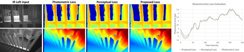
4       Y. Zhang et al.

Fig. 2. ActiveStereoNet architecture. We use a two stage network where a low resolu-
tion cost volume is built and infers the first disparity estimate. A bilinear upsampling
followed by a residual network predicts the final disparity map. An “Invalidation Net-
work” (bottom) is also trained end-to-end to predict a confidence map.

in general scenes [11], suffer from interference and per-camera calibration [12],
and/or do not work well in texture-less areas due to their shallow descriptors
and local optimization schemes [14, 13]. Our paper is the first to investigate how
to design an end-to-end deep network for active stereo.

3     Method

In this section, we introduce the network architecture and training procedure for
ActiveStereoNet. The input to our algorithm is a rectified, synchronized pair of
images with active illumination (see Fig. 1), and the output is a pair of disparity
maps at the original resolution. For our experiments, we use the recently released
Intel Realsense D435 that provides synchronized, rectified 1280 × 720 images at
30fps. The focal length f and the baseline b between the two cameras are assumed
to be known. Under this assumption, the depth estimation problem becomes a
disparity search along the scan line. Given the output disparity d, the depth is
obtained via Z = bf d .
    Since no ground-truth training data is available for this problem, our main
challenge is to train an end-to-end network that is robust to occlusion and illu-
mination effects without direct supervision. The following details our algorithm.

3.1   Network Architecture

Nowadays, in many vision problems, the choice of the architecture plays a crucial
role, and most of the efforts are spent in designing the right network. In active
stereo, instead, we found that the most challenging part is the training proce-
dure for a given deep network. In particular, since our setting is unsupervised,
designing the optimal loss function has the highest impact on the overall accu-
racy. For this reason, we extend the network architecture proposed in [30], which
has shown superior performances in many passive stereo benchmarks. Moreover,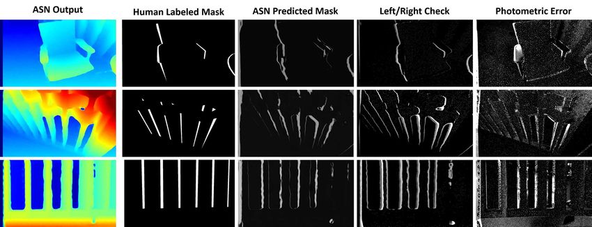
ActiveStereoNet         5

the system is computationally efficient and allows us to run on full resolution at
60Hz on a high-end GPU, which is desirable for real-time applications.
    The overall pipeline is shown in Fig. 2. We start from the high-resolution
images and use a siamese tower to produces feature map in 1/8 of the input
resolution. We then build a low resolution cost volume of size 160 × 90 × 18,
allowing for a maximum disparity of 144 in the original image, which corresponds
to a minimum distance of ∼ 30 cm on the chosen sensor.
    The cost volume produces a downsampled disparity map using the soft
argmin operator [28]. Differently from [28] and following [30] we avoid expen-
sive 3D deconvolution and output a 160 × 90 disparity. This estimation is then
upsampled using bi-linear interpolation to the original resolution (1280 × 720).
A final residual refinement retrieves the high-frequency details such as edges.
Different from [30], our refinement block starts with separate convolution layers
running on the upsampled disparity and input image respectively, and merge the
feature later to produce residual. This in practice works better to remove dot
artifacts in the refined results.
    Our network also simultaneously estimates an invalidation mask to remove
uncertain areas in the result, which will be introduced in Sec. 3.4.

3.2   Loss Function

The architecture described is composed of a low resolution disparity and a final
refinement step to retrieve high-frequency details. A natural choice is to have a
loss function for each of these two steps. Unlike [30], we are in an unsupervised
setting due to the lack of ground truth data. A viable choice for the training
loss L then is the photometric error between the original pixelsP onl the ˆleft   image
 l
Iij and the reconstructed left image Iˆij
                                        l
                                           , in particular L = ij kIij       l
                                                                          − Iij k1 . The
reconstructed image Iˆl is obtained by sampling pixels from the right image I r
using the predicted disparity d, i.e. Iˆij
                                        l        r
                                            = Ii,j−d . Our sampler uses the Spatial
Transformer Network (STN) [26], which uses a bi-linear interpolation of 2 pixels
on the same row and is fully differentiable.
    However, as shown in previous work [57], the photometric loss is a poor
choice for image reconstruction problems. This is even more dramatic when
dealing with active setups. We recall that active sensors flood the scenes with
texture and the intensity of the received signal follows the inverse square law
I ∝ Z12 , where Z is the distance from the camera. In practice this creates an
explicit dependency between the intensity and the distance (i.e. brighter pixels
are closer). A second issue, that is also present in RGB images, is that the
difference between two bright pixels is likely to have a bigger residual when
compared to the difference between two dark pixels. Indeed if we consider image
I, to have noise proportional to intensity [17], the observed intensity for a given
                                 ⋆                ⋆                ⋆
pixel can be written as: Iij = Iij + N (0, σ1 Iij   + σ2 ), where Iij is the noise free
signal and the standard deviations σ1 and σ2 depend on the sensor [17]. It is easy
to show that the difference
                    q        between two correctly matched pixels I and Iˆ has a
residual: ǫ = N (0, (σ1 I + σ2 )2 + (σ3 Iˆ⋆ + σ4 )2 ), where its variance depends
                           ⋆
                            ij               ij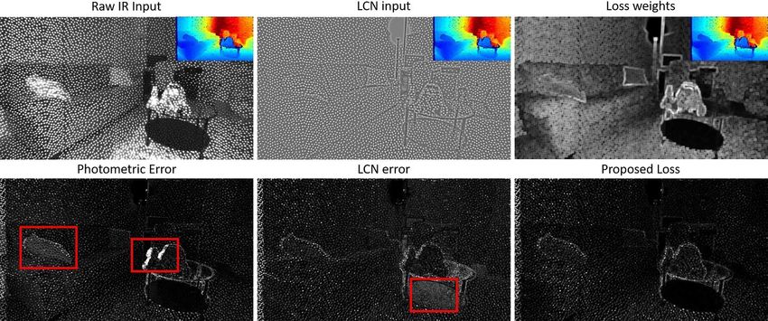
6       Y. Zhang et al.

Fig. 3. Comparisons between photometric loss (left), LCN loss (middle), and the pro-
posed weighted LCN loss (right). Our loss is more robust to occlusions, it does not
depend on the brightness of the pixels and does not suffer in low texture regions.

on the input intensities. This shows that for brighter pixels (i.e. close objects)
the residual ǫ will be bigger compared to one of low reflectivity or farther objects.
    In the case of passive stereo, this could be a negligible effect, since in RGB
images there is no correlation between intensity and disparity, however in the
active case the aforementioned problem will bias the network towards closeup
scenes, which will have always a bigger residual. The architecture will learn
mostly those easy areas and smooth out the rest. The darker pixels, mostly in
distant, requiring higher matching precision for accurate depth, however, are
overlooked. In Fig. 3 (left), we show the the reconstruction error for a given
disparity map using the photometric loss. Notice how bright pixels on the pillow
exhibits high reconstruction error due to the input dependent nature of the noise.
    An additional issue with this loss occurs in the occluded areas: indeed when
the intensity difference between background and foreground is severe, this loss
will have a strong contribution in the occluded regions, forcing the network to
learn to fit those areas that, however, cannot really be explained in the data.

Weighted Local Contrast Normalization. We propose to use a Local Con-
trast Normalization (LCN) scheme, that not only removes the dependency be-
tween intensity and disparity, but also gives a better residual in occluded regions.
It is also invariant to brightness changes in the left and right input image. In
particular, for each pixel, we compute the local mean µ and standard devia-
tion σ in a small 9 × 9 patch. These local statistics are used to normalize the
                                   I−µ
current pixel intensity ILCN = σ+η     , where η is a small constant. The result
of this normalization is shown in Fig. 3, middle. Notice how the dependency
between disparity and brightness is now removed, moreover the reconstruction
error (Fig. 3, middle, second row) is not strongly biased towards high intensity
areas or occluded regions.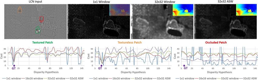
ActiveStereoNet         7

Fig. 4. Cost volume analysis for a textured region (green), textureless patch (orange)
and occluded pixel (red). Notice how the window size helps to resolve ambiguous (tex-
tureless) areas in the image, whereas in occluded pixels the lowest cost will always lead
to the wrong solution. However large windows oversmooth the cost function and they
do not preserve edges, where as the proposed Adaptive Support Weight loss aggregates
costs preserving edges.

    However, LCN suffers in low texture regions when the standard deviation σ
is close to zero (see the bottom of the table in Fig. 3, middle). Indeed these areas
have a small σ which will would amplify any residual together with noise between
two matched pixels. To remove this effect, we re-weight the residual ǫ between
two matched pixel Iij and Iˆij l
                                 using the local standard deviation σij estimated
on the reference image in a 9 × 9 patch  P aroundl the pixel     (i, j). In particular
our reconstruction loss becomes: L = ij kσij (ILCN          − ˆl
                                                              I
                                                                             P
                                                         ij     LCN ij )k1 =    ij Cij .
Example of weights computed on the reference image are shown in Fig. 3, top
right and the final loss is shown on the bottom right. Notice how these residuals
are not biased in bright areas or low textured regions.

3.3   Window-based Optimization
We now analyze in more details the behavior of the loss function for the whole
search space. We consider a textured patch (green), a texture-less one (orange)
and an occluded area (red) in an LCN image (see Fig. 4). We plot the loss
function for every disparity candidate in the range of [5, 144]. For a single pixel
cost (blue curve), notice how the function exhibits a highly non-convex behavior
(w.r.t. the disparity) that makes extremely hard to retrieve the ground truth
value (shown as purple dots). Indeed a single pixel cost has many local min-
ima, that could lie far from the actual optimum. In traditional stereo matching
pipelines, a cost aggregation robustifies the final estimate using evidence from
neighboring pixels. If we consider a window around each pixel and sum all the
costs, we can see that the loss becomes smoother for both textured and texture-
less patch and the optimum can be reached (see Fig. 4, bottom graphs). However
as a drawback for large windows, small objects and details can be smooth out by
the aggregation of multiple costs and cannot be recovered in the final disparity.
    Traditional stereo matching pipelines aggregate the costs using an adaptive
support (ASW) scheme [53], which is very effective, but also slow hence not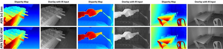
8       Y. Zhang et al.

practical for real-time systems where approximated solutions are required [34].
Here we propose to integrate the ASW scheme in the training procedure, there-
fore it does not affect the runtime cost. In particular, we consider a pixel (i, j)
with intensity Iij and instead of compute a per-pixel loss, we aggregate the costs
                                                    Pi+k−1 Pj+k−1
                                                              y=j−k wx,y Cij
Cij around a 2k × 2k window following: Cˆij = P       x=i−k
                                                        i+k−1 Pj+k−1
                                                                         wx,y
                                                                             , where
                                                         x=i−k   y=j−k
            |I −I |
wxy =  exp(− ijσw xy ),  with σw = 2. As shown in Fig. 4 right, this aggregates
the costs (i.e. it smooths the cost function), but it still preserves the edges. In
our implementation we use a 32 × 32 during the whole training phase. We also
tested a graduated optimization approach [40, 22], where we first optimized our
network using 64 × 64 window and then reduce it every 15000 iterations by a
factor of 2, until we reach a single pixel loss. However this solution led to very
similar results compared to a single pixel loss during the whole training.

3.4   Invalidation Network

So far the proposed loss does not deal with occluded regions and wrong matches
(i.e. textureless areas). An occluded pixel does not have any useful information
in the cost volume even when brute-force search is performed at different scales
(see in Fig. 4, bottom right graph). To deal with occlusions, traditional stereo
matching methods use a so called left-right consistency check, where a disparity
is first computed from the left view point (dl ), then from the right camera
(dr ) and invalidate those pixels with |dl − dr | > θ. Related work use a left-right
consistency in the loss minimization [20], however this leads to oversmooth edges
which become flying pixels (outliers) in the pointcloud. Instead, we propose to
use the left-check as a hard constraint by defining a mask for a pixel (i, j):
mij = |dl − dr | < θ, with θ = 1 disparity. Those pixels with mij = 0 are
ignored in the loss computation. To avoid a trivial solution (i.e. all the pixels
are invalidated), similarly to [59], we enforce a regularization on the number of
valid pixels by minimizing the cross-entropy loss with constant label 1 in each
pixel location. We use this mask in both the low-resolution disparity as well as
the final refined one.
    At the same time, we train an invalidation network (fully convolutional), that
takes as input the features computed from the Siamese tower and produces first
a low resolution invalidation mask, which is then upsampled and refined with a
similar architecture used for the disparity refinement. This allows, at runtime,
to avoid predicting the disparity from both the left and the right viewpoint to
perform the left-right consistency, making the inference significantly faster.

4     Experiments

We performed a series of experiments to evaluate ActiveStereoNet (ASN). In ad-
dition to analyzing the accuracy of depth predictions in comparison to previous
work, we also provide results of ablation studies to investigate how each com-
ponent of the proposed loss affects the results. In the supplementary material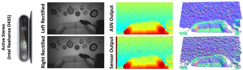
ActiveStereoNet       9

we also evaluate the applicability of our proposed self-supervised loss in pas-
sive (RGB) stereo, showing improved generalization capabilities and compelling
results on many benchmarks.

4.1   Dataset and Training Schema

We train and evaluate our method on both real and synthetic data.
    For the real dataset, we used an Intel Realsense D435 camera [2] to collect
10000 images for training in an office environment, plus 100 images in other
unseen scenes for testing (depicting people, furnished rooms and objects).
    For the synthetic dataset, we used Blender to render IR and depth images of
indoor scenes such as living rooms, kitchens, and bedrooms, as in [14]. Specifi-
cally, we render synthetic stereo pairs with 9 cm baseline using projective tex-
tures to simulate projection of the Kinect V1 dot pattern onto the scene. We
randomly move the camera in the rendered rooms and capture left IR image,
right IR image as well as ground truth depth. Examples of the rendered scenes
are showed in Fig. 8, left. The synthetic training data consists of 10000 images
and the test set is composed of 1200 frames comprehending new scenes.
    For both real and synthetic experiments, we trained the network using RM-
Sprop [49]. We set the learning rate to 1e−4 and reduce it by half at 53 iterations
and to a quarter at 54 iterations. We stop the training after 100000 iterations,
that are usually enough to reach the convergence. Although our algorithm is
self-supervised, we did not fine-tune the model on any of the test data since it
reduces the generalization capability in real applications.

4.2   Stereo Matching Evaluation

In this section, we compare our method on real data with state of the art stereo
algorithms qualitatively and quantitatively using traditional stereo matching
metrics, such as jitter and bias.

Bias and Jitter. It is known that a stereo system with baseline b, focal length
f , and a subpixel disparity precision of δ, has a depth error ǫ that increases
                                                                    2
quadratically with respect to the depth Z according to ǫ = δZ     bf [45]. Due to
the variable impact of disparity error on the depth, naive evaluation metrics,
like mean error of disparity, does not effectively reflect the quality of the esti-
mated depth. In contrast, we first show error of depth estimation and calculate
corresponding error in disparity.
    To assess the subpixel precision of ASN, we recorded 100 frames with the
camera in front of a flat wall at distances ranging from 500 mm to 3500 mm,
and also 100 frames with the camera facing the wall at an angle of 50 deg to
assess the behavior on slanted surfaces. In this case, we evaluate by comparing
to “ground truth” obtained with robust plane fitting.
    To characterize the precision, we compute bias as the average ℓ1 error between
the predicted depth and the ground truth plane. Fig. 5 shows the bias with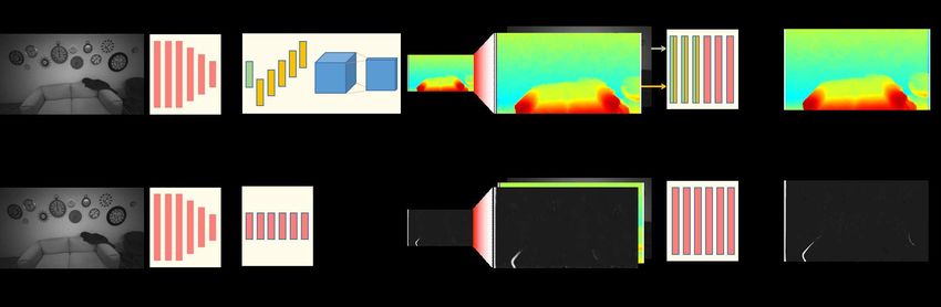
10      Y. Zhang et al.

Fig. 5. Quantitative Evaluation with state of the art. We achieve one order of magni-
tude less bias with a subpixel precision of 0.03 pixels with a very low jitter (see text).
We also show the predicted pointclouds for various methods of a wall at 3000mm dis-
tance. Notice that despite the large distance (3m), our results is the less noisy compared
to the considered approaches.

regard to the depth for our method, sensor output [29], the state of the art
local stereo methods (PatchMatch [7], HashMatch [13]), and our model trained
using the state of the art unsupervised loss [20], together with visualizations
of point clouds colored by surface normal. Our system performs significantly
better than the other methods at all distances, and its error does not increase
dramatically with depth. The corresponding subpixel disparity precision of our
system is 1/30th of a pixel, which is obtained by fitting a curve using the above
mentioned equation (also shown in Fig. 5). This is one order of magnitude lower
than the other methods where the precision is not higher than 0.2 pixel.
    To characterize the noise, we compute the jitter as the standard deviation
of the depth error. Fig. 5 shows that our method achieves the lowest jitter at
almost every depth in comparison to other methods.

Comparisons with State of the Art. More qualitative evaluations of ASN
in challenging scenes are shown in Fig. 6. As can be seen, local methods like
PatchMatch stereo [7] and HashMatch [13] do not handle mixed illumination
with both active and passive light, and thus produce incomplete disparity images
(missing pixels shown in black). The sensor output using a semi-global scheme is
more suitable for this data [29], but it is still susceptible to image noise (note the
noisy results in the fourth column). In contrast, our method produces complete
disparity maps and preserves sharp boundaries.
    More examples on real sequences are shown in Fig. 8 (right), where we show
point clouds colored by surface normal. Our output preserves all the details and
exhibits a low level of noise. In comparison, our network trained with the self-
supervised method by Godard et al. [20] over-smooths the output, hallucinating
ActiveStereoNet 11 Fig. 6. Qualitative Evaluation with state of the art. Our method produces detailed disparity maps. State of the art local methods [7, 13] suffer from textureless regions. The semi-global scheme used by the sensor [29] is noisier and it oversmooths the output. geometry and flying pixels. Our results are also free from the texture copy- ing problem, most likely because we use a cost volume to explicitly model the matching function rather than learn directly from pixel intensity. Even though the training data is mostly captured from office environment, we find ASN gen- eralize well to various testing scenes, e.g. living room, play room, dinning room, and objects, e.g. person, sofas, plants, table, as shown in figures. 4.3 Ablation Study In this section, we evaluate the importance of each component in the ASN sys- tem. Due to the lack of ground truth data, most of the results are qualitative – when looking at the disparity maps, please pay particular attention to noise, bias, edge fattening, flying pixels, resolution, holes, and generalization capabilities. Self-supervised vs Supervised. Here we perform more evaluations of our self-supervised model on synthetic data when supervision is available as well as on real data using the depth from the sensor as supervision (together with the proposed loss). Quantitative evaluation on synthetic data (Fig. 8, left bottom), shows that the supervised model (blue) achieves a higher percentage of pixels with error less than 5 disparity, however for more strict requirements (error less than 2 pixels) our self-supervised loss (red) does a better job. This may indicate overfitting of the supervised model on the training set. This behavior is even more evident on real data: the model was able to fit the training set with high precision, however on test images it produces blur results compared to the self- supervised model (see Fig. 6, ASN Semi Supervised vs ASN Self-Supervised). Reconstruction Loss. We next investigate the impact of our proposed WLCN loss (as described in Sec. 3.2) in comparison to a standard photometric error (L1) and a perceptual loss [27] computed using feature maps from a pre-trained
12      Y. Zhang et al.

Fig. 7. Ablation study on reconstruction loss. Same networks, trained on 3 different
reconstruction losses. Notice how the proposed WLCN loss infers disparities that better
follow the edges in these challenging scenes. Photometric and Perceptual losses have
also a higher level of noise. On the right, we show how our loss achieves the lowest
reconstruction error for low intensity pixels thanks to the proposed WLCN.

VGG network. In this experiment, we trained three networks with the same
parameters, changing only the reconstruction loss: photometric on raw IR, VGG
conv-1, and the proposed WLCN, and investigate their impacts on the results.
    To compute accurate metrics, we labeled the occluded regions in a subset
of our test case manually (see Fig. 9). For those pixels that were not occluded,
we computed the photometric error of the raw IR images given the predicted
disparity image. In total we evaluated over 10M pixels. In Fig. 7 (right), we show
the photometric error of the raw IR images for the three losses with respect to
the pixel intensities. The proposed WLCN achieves the lowest error for small
intensities, showing that the loss is not biased towards bright areas. For the rest
of the range the losses get similar numbers. Please notice that our loss achieves
the lowest error even we did not explicitly train to minimize the photometric
reconstruction. Although the numbers may seem similar, the effect on the final
disparity map is actually very evident. We show some examples of predicted
disparities for each of the three different losses in Fig. 7 (left). Notice how the
proposed WLCN loss suffers from less noise, produces crisper edges, and has a
lower percentage of outliers. In contrast, the perceptual loss highlights the high
frequency texture in the disparity maps (i.e. dots), leading to noisy estimates.
Since VGG conv-1 is pre-trained, we observed that the responses are high on
bright dots, biasing the reconstruction error again towards close up scenes. We
also tried a variant of the perceptual loss by using the output from our Siamese
tower as the perceptual feature, however the behavior was similar to the case of
using the VGG features.

Invalidation Network. We next investigate whether excluding occluded re-
gion from the reconstruction loss is important to train a network – i.e., to achieve
crisper edges and less noisy disparity maps. We hypothesize that the architecture
would try to overfit occluded regions without this feature (where there are no
matches), leading to higher errors throughout the images. We test this quantita-
tively on synthetic images by computing the percentage of pixels with disparity
error less than x ∈ [1, 5]. The results are reported in Fig. 8. With the invalida-
tion mask employed, our model outperforms the case without for all the error
ActiveStereoNet 13
Fig. 8. Evaluation on Synthetic and Real Data. On synthetic data (left), notice how
our method has the highest percentage of pixels with error smaller than 1 disparity.
We also produce sharper edges and less noisy output compared to other baselines. The
state of the art self-supervised method by Godard et al. [20] is very inaccurate near
discontinuities. On the right, we show real sequences from an Intel RealSense D435
where the gap between [20] and our method is even more evident: notice flying pixels
and oversmooth depthmaps produced by Godard et al. [20]. Our results has higher
precision than the sensor output.
threshold (Red v.s Purple curve, higher is better). We further analyze the pro-
duced disparity and depth maps on both synthetic and real data. On synthetic
data, the model without invalidation mask shows gross error near the occlusion
boundary (Fig. 8, left top). Same situation happens on real data (Fig. 8, right),
where more flying pixels exhibiting when no invalidation mask is enabled.
As a byproduct of the invalidation network, we obtain a confidence map
for the depth estimates. In Fig. 9 we show our predicted masks compared with
the ones predicted with a left-right check and the photometric error. To assess
the performances, we used again the images we manually labeled with occluded
regions and computed the average precision (AP). Our invalidation network and
left right check achieved the highest scores with an AP of 80.7% and 80.9%
respectively, whereas the photometric error only reached 51.3%. We believe that
these confidence maps could be useful for many higher-level applications.
Window based Optimization. The proposed window based optimization with
Adaptive Support Weights (ASW) is very important to get more support for thin
structures that otherwise would get a lower contribution in the loss and treated
as outliers. We show a comparison of this in Fig. 10. Notice how the loss with
ASW is able to recover hard thin structures with higher precision. Moreover,
our window based optimization also produces smoother results while preserving
edges and details. Finally, despite we use a window-based loss, the proposed
ASW strategy has a reduced amount of edge fattening.14 Y. Zhang et al. Fig. 9. Invalidation Mask prediction. Our invalidation mask is able to detect occluded regions and it reaches an average precision of 80.7% (see text). Fig. 10. Comparison between single pixel loss and the proposed window based opti- mization with adaptive support scheme. Notice how the ASW is able to recover more thin structures and produce less edge fattening. 5 Discussion We presented ActiveStereoNet (ASN) the first deep learning method for active stereo systems. We designed a novel loss function to cope with high-frequency patterns, illumination effects, and occluded pixels to address issues of active stereo in a self-supervised setting. We showed that our method delivers very precise reconstructions with a subpixel precision of 0.03 pixels, which is one order of magnitude better than other active stereo matching methods. Compared to other approaches, ASN does not oversmooth details, and it generates complete depthmaps, crisp edges, and no flying pixels. As a byproduct, the invalidation network is able to infer a confidence map of the disparity that can be used for high level applications requiring occlusions handling. Numerous experiments show state of the art results on different challenging scenes with a runtime cost of 15ms per frame using an NVidia Titan X. Limitations and Future Work. Although our method generates compelling results there are still issues with transparent objects and thin structures due to the low resolution of the cost volume. In future work, we will propose solutions to handle these cases with high level cues, such as semantic segmentation.
ActiveStereoNet        15

References

 1. Intel realsense d415. https://click.intel.com/intelr-realsensetm-depth-camera-
    d415.html, accessed: 2018-02-28
 2. Intel realsense d435. https://click.intel.com/intelr-realsensetm-depth-camera-
    d435.html, accessed: 2018-02-28
 3. Besse, F., Rother, C., Fitzgibbon, A., Kautz, J.: Pmbp: Patchmatch belief propaga-
    tion for correspondence field estimation. International Journal of Computer Vision
    110(1), 2–13 (2014)
 4. Bhandari, A., Feigin, M., Izadi, S., Rhemann, C., Schmidt, M., Raskar, R.: Re-
    solving multipath interference in kinect: An inverse problem approach. In: IEEE
    Sensors (2014)
 5. Bhandari, A., Kadambi, A., Whyte, R., Barsi, C., Feigin, M., Dorrington, A.,
    Raskar, R.: Resolving multi-path interference in time-of-flight imaging via modu-
    lation frequency diversity and sparse regularization. CoRR (2014)
 6. Bleyer, M., Gelautz, M.: Simple but effective tree structures for dynamic
    programming-based stereo matching. In: VISAPP (2). pp. 415–422 (2008)
 7. Bleyer, M., Rhemann, C., Rother, C.: Patchmatch stereo-stereo matching with
    slanted support windows. In: Bmvc. vol. 11, pp. 1–11 (2011)
 8. Dou, M., Davidson, P., Fanello, S.R., Khamis, S., Kowdle, A., Rhemann, C.,
    Tankovich, V., Izadi, S.: Motion2fusion: Real-time volumetric performance cap-
    ture. SIGGRAPH Asia (2017)
 9. Dou, M., Khamis, S., Degtyarev, Y., Davidson, P., Fanello, S.R., Kowdle, A., Es-
    colano, S.O., Rhemann, C., Kim, D., Taylor, J., Kohli, P., Tankovich, V., Izadi,
    S.: Fusion4d: Real-time performance capture of challenging scenes. SIGGRAPH
    (2016)
10. Fanello, S.R., Gori, I., Metta, G., Odone, F.: Keep it simple and sparse: Real-time
    action recognition. JMLR (2013)
11. Fanello, S.R., Keskin, C., Izadi, S., Kohli, P., Kim, D., Sweeney, D., Criminisi, A.,
    Shotton, J., Kang, S., Paek, T.: Learning to be a depth camera for close-range
    human capture and interaction. ACM SIGGRAPH and Transaction On Graphics
    (2014)
12. Fanello, S.R., Rhemann, C., Tankovich, V., Kowdle, A., Orts Escolano, S., Kim,
    D., Izadi, S.: Hyperdepth: Learning depth from structured light without matching.
    In: CVPR (2016)
13. Fanello, S.R., Valentin, J., Kowdle, A., Rhemann, C., Tankovich, V., Ciliberto,
    C., Davidson, P., Izadi, S.: Low compute and fully parallel computer vision with
    hashmatch (2017)
14. Fanello, S.R., Valentin, J., Rhemann, C., Kowdle, A., Tankovich, V., Davidson, P.,
    Izadi, S.: Ultrastereo: Efficient learning-based matching for active stereo systems.
    In: Computer Vision and Pattern Recognition (CVPR), 2017 IEEE Conference on.
    pp. 6535–6544. IEEE (2017)
15. Fanello, S., Gori, I., Metta, G., Odone, F.: One-shot learning for real-time action
    recognition. In: IbPRIA (2013)
16. Felzenszwalb, P.F., Huttenlocher, D.P.: Efficient belief propagation for early vision.
    International journal of computer vision 70(1), 41–54 (2006)
17. Foi, A., Trimeche, M., Katkovnik, V., Egiazarian, K.: Practical poissonian-gaussian
    noise modeling and fitting for single-image raw-data. IEEE Transactions on Image
    Processing (2008)
16 Y. Zhang et al.
18. Garg, R., BG, V.K., Carneiro, G., Reid, I.: Unsupervised cnn for single view depth
estimation: Geometry to the rescue. In: European Conference on Computer Vision.
pp. 740–756. Springer (2016)
19. Gidaris, S., Komodakis, N.: Detect, replace, refine: Deep structured prediction for
pixel wise labeling. In: Proc. of the IEEE Conference on Computer Vision and
Pattern Recognition. pp. 5248–5257 (2017)
20. Godard, C., Mac Aodha, O., Brostow, G.J.: Unsupervised monocular depth esti-
mation with left-right consistency. In: CVPR. vol. 2, p. 7 (2017)
21. Hamzah, R.A., Ibrahim, H.: Literature survey on stereo vision disparity map al-
gorithms. Journal of Sensors 2016 (2016)
22. Hazan, E., Levy, K.Y., Shalev-Shwartz, S.: On graduated optimization for stochas-
tic non-convex problems. In: ICML (2016)
23. Hirschmuller, H.: Stereo processing by semiglobal matching and mutual informa-
tion. IEEE Transactions on pattern analysis and machine intelligence 30(2), 328–
341 (2008)
24. Hosni, A., Rhemann, C., Bleyer, M., Rother, C., Gelautz, M.: Fast cost-volume fil-
tering for visual correspondence and beyond. IEEE Transactions on Pattern Anal-
ysis and Machine Intelligence 35(2), 504–511 (2013)
25. Ilg, E., Mayer, N., Saikia, T., Keuper, M., Dosovitskiy, A., Brox, T.: Flownet 2.0:
Evolution of optical flow estimation with deep networks. In: IEEE Conference on
Computer Vision and Pattern Recognition (CVPR). vol. 2 (2017)
26. Jaderberg, M., Simonyan, K., Zisserman, A., Kavukcuoglu, K.: Spatial transformer
networks. In: NIPS (2015)
27. Johnson, J., Alahi, A., Li, F.: Perceptual losses for real-time style transfer and
super-resolution. CoRR (2016)
28. Kendall, A., Martirosyan, H., Dasgupta, S., Henry, P., Kennedy, R., Bachrach, A.,
Bry, A.: End-to-end learning of geometry and context for deep stereo regression.
CoRR, vol. abs/1703.04309 (2017)
29. Keselman, L., Iselin Woodfill, J., Grunnet-Jepsen, A., Bhowmik, A.: Intel Re-
alSense Stereoscopic Depth Cameras. CVPR Workshops (2017)
30. Khamis, S., Fanello, S., Rhemann, C., Valentin, J., Kowdle, A., Izadi, S.: Stereonet:
Guided hierarchical refinement for edge-aware depth prediction. In: ECCV (2018)
31. Klaus, A., Sormann, M., Karner, K.: Segment-based stereo matching using belief
propagation and a self-adapting dissimilarity measure. In: Pattern Recognition,
2006. ICPR 2006. 18th International Conference on. vol. 3, pp. 15–18. IEEE (2006)
32. Kolmogorov, V., Zabih, R.: Computing visual correspondence with occlusions using
graph cuts. In: Computer Vision, 2001. ICCV 2001. Proceedings. Eighth IEEE
International Conference on. vol. 2, pp. 508–515. IEEE (2001)
33. Konolige, K.: Projected texture stereo. In: ICRA (2010)
34. Kowalczuk, J., Psota, E.T., Perez, L.C.: Real-time stereo matching on cuda using
an iterative refinement method for adaptive support-weight correspondences. IEEE
Transactions on Circuits and Systems for Video Technology (2013)
35. Kuznietsov, Y., Stückler, J., Leibe, B.: Semi-supervised deep learning for monoc-
ular depth map prediction. In: Proc. of the IEEE Conference on Computer Vision
and Pattern Recognition. pp. 6647–6655 (2017)
36. Liang, Z., Feng, Y., Guo, Y., Liu, H., Qiao, L., Chen, W., Zhou, L., Zhang, J.:
Learning deep correspondence through prior and posterior feature constancy. arXiv
preprint arXiv:1712.01039 (2017)
37. Luo, W., Schwing, A.G., Urtasun, R.: Efficient deep learning for stereo matching.
In: Proceedings of the IEEE Conference on Computer Vision and Pattern Recog-
nition. pp. 5695–5703 (2016)ActiveStereoNet 17
38. Mayer, N., Ilg, E., Hausser, P., Fischer, P., Cremers, D., Dosovitskiy, A., Brox,
T.: A large dataset to train convolutional networks for disparity, optical flow, and
scene flow estimation. In: Proceedings of the IEEE Conference on Computer Vision
and Pattern Recognition. pp. 4040–4048 (2016)
39. Naik, N., Kadambi, A., Rhemann, C., Izadi, S., Raskar, R., Kang, S.: A light trans-
port model for mitigating multipath interference in TOF sensors. CVPR (2015)
40. Neil, T., Tim, C.: Multi-resolution methods and graduated non-convexity. In: Vi-
sion Through Optimization (1997)
41. Nishihara, H.K.: Prism: A practical mealtime imaging stereo matcher. In: Intelli-
gent Robots: 3rd Intl Conf on Robot Vision and Sensory Controls. vol. 449, pp.
134–143. International Society for Optics and Photonics (1984)
42. Pang, J., Sun, W., Ren, J., Yang, C., Yan, Q.: Cascade residual learning: A two-
stage convolutional neural network for stereo matching. In: International Conf. on
Computer Vision-Workshop on Geometry Meets Deep Learning (ICCVW 2017).
vol. 3 (2017)
43. Scharstein, D., Szeliski, R.: A taxonomy and evaluation of dense two-frame stereo
correspondence algorithms. International journal of computer vision 47(1-3), 7–42
(2002)
44. Shaked, A., Wolf, L.: Improved stereo matching with constant highway networks
and reflective confidence learning. CoRR, vol. abs/1701.00165 (2017)
45. Szeliski, R.: Computer Vision: Algorithms and Applications. Springer-Verlag New
York, Inc., New York, NY, USA, 1st edn. (2010)
46. Tankovich, V., Schoenberg, M., Fanello, S.R., Kowdle, A., Rhemann, C., Dzitsiuk,
M., Schmidt, M., Valentin, J., Izadi, S.: Sos: Stereo matching in o(1) with slanted
support windows. IROS (2018)
47. Taylor, J., Bordeaux, L., Cashman, T., Corish, B., Keskin, C., Sharp, T., Soto, E.,
Sweeney, D., Valentin, J., Luff, B., Topalian, A., Wood, E., Khamis, S., Kohli, P.,
Izadi, S., Banks, R., Fitzgibbon, A., Shotton, J.: Efficient and precise interactive
hand tracking through joint, continuous optimization of pose and correspondences.
SIGGRAPH (2016)
48. Taylor, J., Tankovich, V., Tang, D., Keskin, C., Kim, D., Davidson, P., Kowdle,
A., Izadi, S.: Articulated distance fields for ultra-fast tracking of hands interacting.
Siggraph Asia (2017)
49. Tieleman, T., Hinton, G.: Lecture 6.5-rmsprop: Divide the gradient by a running
average of its recent magnitude. In: COURSERA: Neural Networks for Machine
Learning (2012)
50. Wang, S., Fanello, S.R., Rhemann, C., Izadi, S., Kohli, P.: The global patch collider.
CVPR (2016)
51. Xie, J., Girshick, R., Farhadi, A.: Deep3d: Fully automatic 2d-to-3d video conver-
sion with deep convolutional neural networks. In: European Conference on Com-
puter Vision. pp. 842–857. Springer (2016)
52. Yoon, K.J., Kweon, I.S.: Locally adaptive support-weight approach for visual cor-
respondence search. In: Computer Vision and Pattern Recognition, 2005. CVPR
2005. IEEE Computer Society Conference on. vol. 2, pp. 924–931. IEEE (2005)
53. Yoon, K.J., Kweon, I.S.: Adaptive support-weight approach for correspondence
search. PAMI (2006)
54. Zagoruyko, S., Komodakis, N.: Learning to compare image patches via convolu-
tional neural networks. In: Computer Vision and Pattern Recognition (CVPR),
2015 IEEE Conference on. pp. 4353–4361. IEEE (2015)18 Y. Zhang et al.
55. Zbontar, J., LeCun, Y.: Computing the stereo matching cost with a convolutional
neural network. In: Proceedings of the IEEE conference on computer vision and
pattern recognition. pp. 1592–1599 (2015)
56. Zbontar, J., LeCun, Y.: Stereo matching by training a convolutional neural network
to compare image patches. Journal of Machine Learning Research 17(1-32), 2
(2016)
57. Zhao, H., Gallo, O., Frosio, I., Kautz, J.: Loss functions for image restoration with
neural networks. IEEE Transactions on Computational Imaging (2017)
58. Zhong, Y., Dai, Y., Li, H.: Self-supervised learning for stereo matching with self-
improving ability. arXiv preprint arXiv:1709.00930 (2017)
59. Zhou, T., Brown, M., Snavely, N., Lowe, D.G.: Unsupervised learning of depth and
ego-motion from video. In: CVPR. vol. 2, p. 7 (2017)You can also read