Energy Harvesting Long-Range Marine Communication - Faculty
←
→
Page content transcription
If your browser does not render page correctly, please read the page content below
Energy Harvesting Long-Range Marine
                          Communication
    Ali Hosseini-Fahraji, Pedram Loghmannia, Kexiong Zeng, Xiaofan Li, Sihan Yu, Sihao Sun, Dong Wang,
                                  Yaling Yang, Majid Manteghi, and Lei Zuo
             Bradley Department of Electrical and Computer Engineering, Virginia Tech, Blacksburg, VA, USA
                {alih91, pedraml, kexiong6, lixf, shy, sihaosun, dong0125, yyang8, manteghi, leizuo}@vt.edu

   Abstract—This paper proposes a self-sustaining broadband          size of a webpage is more than 2 MB [4] and is still growing,
long-range maritime communication as an alternative to the           even common web-browsing is painfully slow through this
expensive and slow satellite communications in offshore areas.       technology. The second option is MF, HF, or VHF ship-
The proposed system, named Marinet, consists of many buoys.
Each of the buoys has two units: an energy harvesting unit and a     to-shore radios, which only support voice communications
wireless communication unit. The energy harvesting unit gener-       because of their limited bandwidth (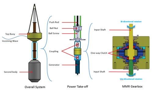
low-maintenance, which can be mass-produced and dropped in balloon control causes mid-air collision with other aircraft,
into water with low deployment cost. The buoy can harvest unwanted balloon landings affecting human life, and unpre-
energy from the ocean wave by taking advantage of the relative dictable landing places for future maintenance. In addition,
motion between the floating buoy and the submerged body, predicting balloon routes and monitoring balloons in real-time
which provides the energy source to support the wireless motion require a huge database and complex programming to
communication services of the base-station. The base-station generate mesh networking and provide reliable communica-
on a buoy maintains high-speed wireless connections with tion. The Aquila project intends to use solar-powered drones
neighboring buoys, which form a self-organized mesh net- as relay stations. However, it was halted after 4 years in June
work. The mesh network is connected to gateways, which 2018 because landing the super-sized Aquila drones turned out
have high-speed fiber connections to the Internet and can to be a huge challenge.
either be mounted on the shore or any fixed infrastructures
in the ocean. The buoys are anchored to the seafloor to ensure III. E NERGY H ARVESTING B UOY
the stability of the mesh network. In this way, we can solve The energy harvesting buoy is the cornerstone of the entire
the challenges of base-station placement and power supply system, since using long cables to access land power is
by using floating base-stations and energy harvested from the extremely costly. Although solar power is easy to harvest, it
ocean. Meanwhile, by leveraging multi-hop wireless links, the is not stable due to night time, weather, and seasonal factors.
lack of cable connection is resolved. Therefore, combining the In addition, when operating in the ocean, solar panels require
floating base-stations, sustainable power harvested from the regular cleaning due to the growth of marine organisms (e.g.,
ocean, and multi-hop wireless links, Marinet can provide low- barnacles, algae, etc.) on them. Thus, in our work, we designed
cost, high-speed connectivity to various maritime applications. ocean-wave energy harvesting units for the buoys so that our
Such a wireless mesh network covering offshore areas will buoys can consistently harvest large enough amounts of power
satisfy the vast majority of the communication needs for ships to support communication services. By measurements taken
and oil platforms in the ocean. in both the ocean and wave tank, the buoy is predicted to
The purpose of this paper is to provide a proof of concept for continuously generate electrical power in tens or hundreds of
such a Marinet system by developing and evaluating the key watts from ocean waves (e.g., 76–306 W for 0.5–1 m wave
units of such a system. Specifically, a brief description of the height that falls into sea state 2–3). Moreover, wave energy
energy harvesting buoy and its expected power generation is is very stable compared to solar panels and less affected by
presented in Section III. Section IV is dedicated to the design light/weather conditions. With such a high and stable energy
of wireless radios for marine communications. Then, the chal- supply, energy harvesting buoys can provide sustainable power
lenges and their feasible solutions in the mesh network design to networking devices. Also, since the energy harvesting unit
are considered in Section V. The evaluation of the system is enclosed in a water-tight case, it will not suffer from the
based on field measurement data and simulation is discussed growth of marine organisms and hence is low-maintenance.
in Section VI. This paper is concluded in Section VII.
A. Design and Testing of the Two-Body Self-React Ocean
II. R ELATED W ORK Wave Energy Converter
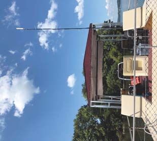
Some of the recent efforts to address marine communication As shown in Fig. 1, the energy harvesting unit known as
problems include the Google Loon project and the Facebook wave energy converter (WEC) contains two bodies: a floating
Aquila project. The Loon project attempts to provide internet buoy moving up and down with ocean waves, and a submerged
connectivity through mesh networks formed by balloons. Yet, body in a certain ocean depth. The bi-directional up and
it faces severe safety and reliability issues. The balloons have a down motions of the floating buoy converts into uni-directional
short life span of 100 days and move by wind currents. Failure motions to drive the generator to produce electricity. Fig. 2
illustrates the design of the WEC, which is designed to achieve
%DFNKDXO/LQNEHWZHHQ%XR\V
the self-react effect and catch up with the low excitation
$FFHVV/LQNWR(QG8VHUV frequency of the ocean wave. The theoretical analysis and
$QWHQQD
detailed description of the two-body design can be found in
[7], [8]. This two-body system has a relative heave motion
:DWHU3URRI
ǭ :KLWH6SDFH5RXWHU under wave excitation, which is directly transferred through
ǭ %XR\ a set of the ball screw and ball nut into the power take-
off (PTO). Based on a mechanical motion rectifier (MMR)
(QHUJ\+DUYHVWLQJ8QLW
mechanism, the power take-off can rectify the reciprocating
rotation of the ball screw into a single directional rotation, then
drive a permanent-magnetic generator to provide the electricity
that power other devices [9]. Through dry laboratory tests, as
shown in Fig. 3, we identified and characterized the overall
WEC with the MMR PTO, where an accurate model between
the harvested energy and the water surface displacement is
Fig. 1. Illustration of Marinet.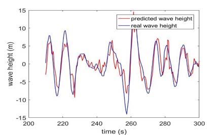
Bi-directional Rotation
                            Push Rod

                              Ball Nut
                                                          Input Shaft
   Top Buoy                 Ball Screw                                                                                                           Ball Screw
                                                                                                      Power Take-off
Incoming Wave
                                                                                                        Electric Load
                            Coupling                       One-way
                                                                                                                                                 Ball Screw Nut
                                                                                                          Ball Screw
                                                            Clutch
                                                                                                   Hydraulic Actuator
                            Generator                                                                                                           MMR Gearbox

Second Body                                               Input Shaft
                                                                                                                                                Generator
                                                                        Uni-directional Rotation

           Overall System                Power Take-off                 MMR Gearbox                      Fig. 3. Dry lab testing of the PTO prototype.            Fig. 4. Water tank test.

                Fig. 2. Design details of the WEC and PTO.

established. We then compare the model with real test results                                                   (offshore point (39.689934, -74.016235)) shows that 132 MHz
in a water tank, as illustrated in Fig. 4, where a series of                                                    bandwidth is available on the TV white space band, while in
waves with specified wave parameters are generated. Fig. 5                                                       Philadelphia, the terrestrially available TV white space is only
compares the water tank test results with simulations that                                                      42 MHz. The amount of TV white space in the offshore area is
are based on the characterization model. Our model matches                                                      significant regarding communication capacity since the entire
well with real test results, indicating that through reasonable                                                 2.4 GHz Wi-Fi band has only 100 MHz spectrum, and cell
system identification and characterization, the performance of                                                   phone providers such as Verizon Wireless rely on a mere 114
the proposed WEC can be well predicted. Since wave power is                                                     MHz spectrum to provide broadband wireless service [13].
proportional to the wave height square and wave period, with                                                       2) Greater Coverage Distance: Compared to other broad-
sufficient knowledge of the wave coming to the WEC, the total                                                    band communication frequencies, TV white space signals
energy to be generated can be forecast, and pre-planning for                                                    can transmit over longer distances because they operate at
the power usage is applicable [10].                                                                             lower frequencies (typically, 470–698 MHz). Specifically, for
                                                                                                                the same transmit power and antenna gain, the white space
B. Average Power Generation Analysis
                                                                                                                band coverage distance is four or five times further than
   Given the model of our WEC mentioned in Subsec-                                                              2.4 GHz Wi-Fi signal. For example, the tens-of-kilometer
tion III-A, based on the profile of real ocean waves, we                                                         transmitted range is achieved in practical white space network
can estimate the maximum, average, and minimum energy                                                           deployment on the land [14]–[16]. With greater coverage
that can be generated for a given time period in the ocean.                                                     distance, the number of nodes in the mesh network can be
Specifically, the wave profile shown in Fig. 6 is acquired from                                                   reduced. Therefore, a target area can be covered by less energy
the NOAA buoy center [11], which shows the significant wave                                                      harvesting buoys and mesh routers, so that the manufacturing
heights over a year. Here, significant wave height is a physical                                                 and deployment cost is reduced significantly.
oceanographic term representing the mean wave height of the                                                        However, commercial off-the-shelf white space radios are
highest third of the waves. Based on the wave profile data,                                                      expensive ($4000–$5000 for a base-station and $1000–$2000
the dominant wave period is obtained from the frequency                                                         for a client [17]) and also not power-efficient (e.g., for 0.2 W
domain analysis, and the power generation over 365 days is                                                      transmit power consumes 25 W of power [18]). The high cost
then estimated, as shown in Fig. 7. The average harvested                                                       and power significantly limit the scalability of the network
power is 57.7 W, which is much more than the 12 W peak                                                          and make the practical deployment unlikely. Moreover, since
power consumption of our communication unit, which will be                                                      commercial white space radio hardware and software are pro-
discussed in the next section.                                                                                  prietary, customizing them to the proposed Marinet application
         IV. W HITE S PACE ROUTER I MPLEMENTATION                                                               is tedious. Therefore, we have designed and implemented a
                                                                                                                low-cost, low-power white space router prototype, which is
   Our communication units on all the buoys essentially act as                                                  customized for use on the ocean. Specifically, we integrated a
wireless routers in a mesh network. Ideally, such a router on                                                   compact 2.4 GHz low-power Wi-Fi router with an RF front-
the ocean should support high-speed links, have large coverage                                                  end to convert the 2.4 GHz frequency signal of the Wi-Fi
distance, and be low-cost and low-power. In our work, we built                                                  output to a TV white space band. A light-weight omnidirec-
wireless mesh routers that operate on the TV white space band                                                   tional antenna has been designed to transmit/receive signals at
for two reasons.                                                                                                the TV white space band. The peak power consumption of the
   1) Large Communication Capacity: Although the center                                                         prototyped system is only 12 W for 0.32 W transmit power
frequency of the TV white space is one-fifths of the Wi-                                                         and 15 W for 0.5 W transmit power.
Fi band, the available bandwidth in the TV white space is
wider than Wi-Fi in the offshore area. For example, the query                                                   A. RF Front-End
result from Google’s TV white space database [12] for an off-                                                     The main function of the RF front-end is down-conversion
shore location 8.4 km away from the shore near Philadelphia                                                     and up-conversion between Wi-Fi and white space bands.
Time domain result of the WEC 3.5
Displacement (m) 0.05
Significant Wave Height(m)
Test results 3
0 Simulation results
2.5
-0.05 2
210 212 214 216 218 220 222 224 226 228 230 1.5
Time (s)
1
5 Test results 0.5
Voltage (V)
Simulation results 0
0 100 200 300
Days
0
210 212 214 216 218 220 222 224 226 228 230
Time (s)
Fig. 6. The wave profile of site 44099 Fig. 7. The Simulated transient power
which is about 20 Km away from the and average power of the WEC during a
Fig. 5. Test results vs. simulation results of the water tank test. coast of Virginia Beach in 2017. year.
The simplest form of up/down-conversion is implemented to inertial measurement unit (accelerometer, gyroscope, and mag-
reduce the overall size and cost. In addition, to increase the netometer), and barometric pressure sensors. This kit monitors
communication range, a power amplifier and a low noise the ocean environment by providing information such as real-
amplifier (LNA) are incorporated in the transmit and receive time motion, temperature, humidity, and pressure. A Raspberry
sides, respectively. Fig. 8 shows the detailed block diagram Pi as a microcomputer connected to a camera streams surveil-
of the RF front-end. As depicted, two mixers are used in the lance video to the router via Ethernet cable. The total cost for
transmitter (top path) and receiver (bottom path) for down- the prototype is around $523, which is ten times cheaper than
conversion and up-conversion, respectively. The router board the commercial off-the-shelf white space routers. This low-
used in this project has two pins: the first one is an input/output cost white space router significantly reduces the deployment
for 2.4 GHz RX/TX-RF signal, and the second one is a cost of the proposed maritime mesh network. Moreover, the
digital pin specifying the status of the board (low for transmit prototyped router supports high transmission power (currently
mode and high for receive mode). To use a single antenna set at 25 dBm) for long-distance communication. Measurement
in both transmit and receive modes, an RF switch is utilized results show the maximum power consumption of the entire
to separate the transmit and receive paths. The switch is router is only 12 W when the RF transmit power is set to
controlled by the digital pin of the router board. In the transmit 25 dBm, which is less than half the power consumed by
side, the router RF pin is connected to a variable attenuator commercial off-the-shelf white space routers. It provides a
to adjust the signal level before feeding it to the mixer. After large margin of power budget, given the power harvested by
mixing the signal with a local oscillator (PLL board locked at the energy harvesting unit. These results confirm the feasibility
1.959 GHz), it is amplified using a driver amplifier followed of our white space router for the energy harvesting mesh net-
by a power amplifier. The maximum power delivered to the work application. It worth mentioning that the Sleeve Dipole
antenna port is 0.5 W. Low-pass, and band-pass filters are antenna as a simple, low-cost, and low-weight structure is used
implemented to suppress unwanted harmonics. On the other for link communication. This antenna has an omnidirectional
hand, on the receive side, before up-converting the signal, the pattern with 2 dBi gain, and it can be replaced by a higher
LNA is used to increase the received signal level. Then, the up- gain antenna [19] to improve the performance of the link.
converted signal is connected directly to the router board. To The router runs a customized version of OpenWrt [20],
make the overall structure small, multilayer PCB technology which is an open-source Linux distribution for embedded
is used in the design of the RF front-end. The overall size of devices. OpenWrt provides an interface for flexible chan-
the board is 6.1 cm × 4.75 cm, and its input voltage is 7 V. nel bandwidth configurations of 5, 10, and 20 MHz, which
can appropriately fit into TV channels with 6 MHz band-
B. White Space Router width/channel.
As shown in Fig. 10, our low-cost and low-power TV white
V. M ARITIME M ESH N ETWORKING
space router prototype includes seven sub-circuits: the RF
front-end, a 2.4-GHz Wi-Fi router, a PLL, a microcontroller, As mentioned in Section III and Section IV, the prototypes
a sensor kit, a microcomputer connected to a camera, and of the energy harvesting unit and the wireless router unit
an antenna. In the transmitter side, the output signal of the maintain the feasibility for broadband connection between two
Wi-Fi router at 2.4 GHz is fed into the RF front-end. The remote buoys. Nevertheless, in order to guarantee the stable
signal is down-converted into a specific available white space operation of a large mesh network, the way of handling the
band and then transmitted. On the receiver side, the RF front- link stability issue under rough sea states is a critical challenge
end up-converts the received signal at the white space band for Marinet.
to the 2.4 GHz frequency band, and after filtering, delivers
the signal to the Wi-Fi router. The microcontroller receives A. Stability Challenges for Marinet
commands from the router to control the PLL for dynamic Compared with traditional terrestrial mesh networks, one
channel selection in the TV white space band. It also controls unique challenge for Marinet is the intrinsic link dynamics
the sensors to send real-time streaming data back to the router under rough weather situations. On land, the mesh nodes are
for processing. The sensor kit includes a GPS receiver, an usually mounted on the roof of tall buildings. Hence, theyRF-Front End
Digital pin
Mixer
Ant.
TX-Port Power
2.432 GHz PD RF
RF LPF Amp. LPF
Amp.
Att. LO
RX-Port (a) Communication link is on.
Sw Pin Tx/Rx Pin
SW 473 MHz
PD
BPF
Router Board (AR9344) LO-Port Ant-Port
LO
BPF RF LNA
PLL Board
Att.
(HMC832) 1.959 GHz (b) Communication link is off.
Fig. 9. Unstable communication link caused
Fig. 8. RF front-end block diagram. by a dynamic ocean wave.
Regular
on link-state prediction [21]. These existing prediction-based
2.4 GHz RF Antenna
Wi-Fi Router TX/RX Fornt-End
TX/RX routing/scheduling schemes are often found in the fields of mo-
Users Board 2.4 GHz 470-698 MHz
bile ad hoc networks and vehicular ad hoc networks, although
7v
12 V
UART
Sensor
their link-state prediction part is not applicable in marine
5.5 V Environment
PLL Kit networks. Thus, by integrating our marine link-state predic-
5.5 V
tion algorithm with these existing adaptive routing/scheduling
Power DC-to-DC
Supply Convertor 5V Microcontroller schemes, we can make them applicable to Marinet.
(a) White space router schematic.
B. Measurement of Buoy Height
RF Front-End
DC-to-DC
A low-cost accelerometer is integrated into every buoy to
2.4 GHz WiFi
Converter measure buoy displacement. Since accelerometer can only
Router
Sensor Kit
measure acceleration instead of displacement, we compute the
A Pen integral of acceleration to obtain speed and then calculate the
(for size reference) PLL integral of speed to obtain displacement.
Microcontroller Due to inaccuracies in accelerometer measurement, during
Raspberry Pi (Arduino Mega)
+ Camera these two integrations, errors will be accumulated and ampli-
fied, resulting in the drift of final buoy displacement result
that completely overshadows the real movement of buoys, as
(b) Prototyped white space router.
shown by the ”displacement before filtering” subfigure in Fig.
Fig. 10. White space router. 11. To address this problem, through spectrum analysis, we
can maintain stable line-of-sight communication links between discovered that the drift in displacement is dominated by low
each other. However, small-sized floating buoys cannot support frequencies. Thus, we applied a high pass digital filter to filter
such high antennas due to physical stability requirements. out the low-frequency signals in 0-0.1 Hz. We tested the results
Therefore, as the ocean becomes rough, the communication of the filtering using an oscillation generator so that we could
links are affected by the instant heights of both the trans- compare the filtered results with the ground truth provided by
mitting/receiving antennas and the waves between them, as the oscillation generator. The filtering algorithm works very
shown in Fig. 9. This situation might cause quality degradation well, as shown in Fig. 11, where the ground truth of oscillation
or even temporary blockage for the communication links. In matches perfectly with the displacement sensing data after the
a mesh network, such unstable links can cause long packet filtering.
delays and also affect the convergence of routing algorithms.
Without carefully designed solutions, the entire mesh network C. Prediction of Buoy Heights
might not work under rough sea states. According to the history of buoy displacement measure-
In order to handle this challenge, we developed a link-state ments, our algorithm then predicts the future of buoy displace-
prediction algorithm for Marinet. Briefly speaking, the algo- ment using an appropriate machine learning algorithm. Our
rithm derives the buoy heights based on the sensor readings. selection of the best learning algorithm is not blind. Instead,
Using the historical and current buoy height measurements, assuming that the buoy movement is the same as the movement
machine learning techniques are applied to predict antenna of ocean surface displacement, we conduct a formal analysis
height in the next few seconds, which are then converted to of ocean waves to identify the proper learning algorithm.
link-state prediction. In this section, we describe the details of First, we observe that oceanography studies have already
the link-state prediction algorithm. revealed that ocean waves can be described by the linear
It is important to note that our contribution focuses on the wave theory, which is widely accepted as an accurate model
marine link-state prediction algorithm. We argue that there of ocean waves in deep water based on extensive real-world
are already numerous existing adaptive routing and scheduling wave measurement data [22]–[25]. It states that the stochastic
algorithms that make their routing/scheduling decisions based process of ocean surface displacement at a given location candisplacement (m) original oscillation
0.05
0
-0.05
0 1 2 3 4 5 6 7 8 9 10
time (s)
displacement (m)
displacement before filtering
2
0 Fig. 12. Real ocean surface movement measurement from [26], which was
-2 originally supplied by M. Olagnon, IFREMER, France, and P. Palo, US Naval
-4 Facilities Engineering Service Center.
0 1 2 3 4 5 6 7 8 9 10
time (s)
displacement (m)
displacement after filtering
0.05
0
-0.05
0 1 2 3 4 5 6 7 8 9 10
time (s)
Fig. 11. Filtered sensing results vs. ground truth of displacement (labeled as
original oscillation)
be modeled as a linear combination of independent sinusoid
waves as follows:
n Fig. 13. Prediction accuracy of the multiple linear regression model.
F (t) = i=1 Ai sin(ωi t + θi ), (1)
where t is time. Random variables θi , wi , and Ai represent M dimensional basis C = {F (t − k)|k ∈ {0, 1, ..., M }}.
different phases, frequencies, and amplitudes of the sinusoid Since M >> n, basis B is a subset of basis C. According to
waves, respectively. We can simplify the above expression as linear algebra’s change of basis computation, the future ocean
n
F (t) = i=1 Ai fi (t), wherefi (t) = sin(ωi t + θi ). (2) surface displacement, hence, can be expressed by basis C as:
Assuming the current time is t, samples of the past history M
F (t + δ) = wk (δ)F (t − k), (7)
of F (t) can be expressed as: k=0
n
F (t − k) = i=1 Ai fi (t − k) for k ∈ {0, 1, ..., M } where wk (δ) are some unknown coefficients. Equation (7) is
(3) the standard relationship where the fast and simple multiple
where is the sampling interval of the history, and M is the linear regression method can be applied so that historical data
total number of samples. In addition, note that a single sinusoid of F (t) is used to learn wk . We also vary different values
has the following property: of and M during the training process to find the optimal
sample interval () and sampling number (M ) based on the
sin(wi (t + δ) + ki x + θi ) = cos(ωi δ) sin(ωi t + ki x + θi ) past history of F (t).
π
+ sin(ωi δ) sin(ωi (t − ) + ki x + θi ). (4) Using the above multiple linear regression method, we are
2ωi
able to build a very simple and accurate prediction model for
⇐⇒ fi (t + δ) = αi (δ)fi (t) + βi (δ)fi (t − γi ) (5) displacement. Fig. 12 shows the 300 seconds of real ocean
where αi (δ) = cos(wi δ), βi (δ) = sin(wi δ), and γi = 2w π
i
. wave movement data. We divide the data into two parts.
Combining (5) with (2), the future of ocean surface displace- The first 200 s of data is used to train the multiple linear
ment at a fixed point can be expressed as: regression model to obtain wk , , and M and the last 100 s
n data is used to test the model’s performance. The prediction
F (t+ δ) = i=1 Ai fi (t + δ) lead time δ is set to 5 s. Fig. 13 shows the prediction
n n
= i=1 Ai αi (δ)fi (t) + i=1 Ai βi (δ)fi (t − γi ) (6) results. Table I further compares the prediction accuracy of
n n
≈ i=1 Ai αi (δ)fi (t) + i=1 Ai βi (δ)fi (t − ki ), our algorithm, marked as mlr (multiple linear regression), with
where we assume M is large enough and is fine enough a few neural network algorithms and a harmonic regression
such that every γi in (6) can find a corresponding integer ki algorithm under different prediction lead time (δ) setting. The
such that ki ≈ γi . We can treat the set of all fi (t − ki ) prediction accuracy is measured by the Pearson correlation
and fi (t) in (6) as a basis of a 2n dimensional vector coefficient, where a value of 1 means a perfect match between
space, a.k.a. B = {fi (t − ki ), fi (t)|i ∈ {0, 1, ..., n}}. With predictions and actual values. As can be seen, since our mlr-
such an interpretation, (6) shows that the future of ocean based prediction algorithm is selected based on a proven model
surface displacement is a linear combination of the basis B. of ocean wave movements, its performance is persistently
Equation (3) shows the relationship between B and another much better than the other machine learning options.TABLE I Relationship between nod elevation and Relationship between nod elevation and
P REDICTION ACCURACY ( THE CORRELATION COEFFICIENT BETWEEN link stability when the sea state is 4 link stability when the sea state is 5
(wind speed is 12 m/s) (wind speed is 15 m/s)
PREDICTION AND REAL VALUE *100%) OF OCEAN SURFACE 5 5
1.0 link stability
DISPLACEMENT [27] 4 0.9 link stability 4
3 0.7 link stability 3
0.5 link stability
δ 2 2
RX elevation
RX elevation
Method 1 1
5s 8s 10s 13s 15s
0 0
mlr 90.95 87.59 83.25 76.15 72.41 -1 -1
elman 87.31 82.26 75.28 68.59 61.47 -2 -2
newff 81.05 77.82 73.59 66.77 61.06 -3 -3 1.0 link stability
0.9 link stability
cascadeforwardnet 84.91 80.73 74.64 66.94 61.16 -4 -4 0.7 link stability
0.5 link stability
newfftd 73.79 66.15 62.17 52.33 46.83 -5 -5
-5 0 5 -5 0 5
newgrnn 70.89 63.47 57.36 46.27 38.62 TX elevation TX elevation
newrb 54.45 49.61 46.51 37.82 32.63
newrbe 40.81 34.18 31.83 22.7 15.8 (a) wind speed = 12 m/s (b) wind speed = 15 m/s
harmonic regression 24.06 21.38 19.24 15.88 12.05
Fig. 14. Relationship between transmitter/receiver heights and link stability
in different sea states. Link stability = 1 − link blocking probability and link
distance=5km.
D. Link-State Prediction Based on Buoy Heights
With the predicted buoy displacement information, the next where C is a scaling constant, g is the gravitational constant,
step is to map this information to link-state prediction. In this V is the wind speed, and d is the wind direction.
work, we use ocean wave simulation to find out the relation- Through the above semi-empirical ocean surface simulation,
ship between buoy displacement and link status. Specifically, we are able to create dynamic and realistic ocean surface
we assume that the communication link between two buoys movements between a pair of buoys. We then use the ocean
is broken if the sea surface between them blocks the line-of- surface simulations to estimate the relationship between buoy
sight link between them. Then, a realistic simulator of ocean heights and link stability. Fig. 14 shows the simulation results
waves in both the time and space domain can provide statistics for 12 m/s and 15m/s wind speeds, where the probability
of such link break probability corresponding to different buoy that the link is alive with respect to different transmitter and
distance, buoy heights, and the long-term wind speed. receiver heights are shown. It can be seen that the link stability,
In our study, we use the semi-empirical method outlined in as shown in Fig. 14, is a function of the elevation of the
[28] to create realistically simulated ocean waves between a transmitter and receiver as well as the wind speed. When two
pair of buoys. The first step is to build an ocean wave model communicating buoys’ heights are in the upper right corner
for a Lx × Ly rectangular ocean area. Note that according area enclosed by the 1.0 link stability line, the communication
to linear wave theory, for a location x = (x, y) in this area, link is fairly stable and has no risk of link breaks.
its ocean surface displacement at time t, denoted as F (x, t), The simulation-derived function that maps transmit-
can be represented as the sum of sinusoids with complex and ter/receiver heights to link stability can be computed offline
time-independent amplitudes: and stored at each buoy as a look-up table. Then, a buoy can
predict its future link-state by searching the link stability value
F (x, t) = Re{ k F (k, t) exp(ikx)}, (8) corresponding to the predicted future heights of itself and its
where k is a two-dimensional vector k = (kx , ky ), kx = communication peer.
2πn/Lx , ky = 2πm/Ly , −N/2 ≤ n ≤ N/2, and −M/2 ≤
m ≤ M/2. Given the spectrum expression of ocean wave VI. E VALUATION
F (k, t), the temporal ocean surface displacement F (x, t)
can be computed by IFFT (inverse fast Fourier transform) We used both field experiments and simulations to evaluate
algorithm. Demonstrated by statistical analysis of real ocean various units of the Marinet. The field experiment focused on
monitoring data, F (k, t) are nearly statistically stationary, a single link performance in a small-scale two-buoy scenario.
independent, Gaussian fluctuations. Mathematically, The simulation was used to examine the performance of a
large-scale ocean mesh network.
F (k, t) = A(k)
exp(iωt) + A∗ (−k) exp(−iωt), (9)
A. Link Measurement
where ω = g|k| in deep water and ∗ is the conjugate
operation. A(k), which are the Fourier amplitudes of a wave In this section, the measurement results for single-link
height field, are expressed by: performance on the water are described. The measurements
√ represent the performance of access links, including received
A(k) = 1/ 2(ξr + iξi ) P (k), (10)
signal strength and throughput over a range of distance. By
where ξr and ξi are independent random numbers with a comparing the measured data with theoretical models, we find
Gaussian distribution N (0, 1). Empirical analysis of real ocean a path loss exponent, which can cursorily determine the range
data has shown that: and reliability of the mesh links. Furthermore, we introduce
2
an empirical mapping between signal power and achievable
P (k) = C
|k|4 exp( |k|−g k
2 V 4 )( |k| d), (11) throughput to evaluate the throughput of the single-link.White
Antenna Space TABLE II
with 5m Router NS3 S IMULATION PARAMETERS .
Rod
Transmission power 25 dBm
Battery
Pack Transmitter/receiver gain 10 dBi
Height of antenna 5m
Packet configuration 100 pkt/s, 1200Bytes/pkt
Node distance 5000 m
Total simulation time 45 s
Transport Layer UDP
Network Layer IP & OLSR or our routing protocol
Data-link Layer Spatial TDMA, 802.11g
20MHz Bandwidth OFDM
Physical Layer
Center Frequency: 600 MHz
Fig. 15. Experiment setup for field measurements.
1) Experiment Setups: Fig. 15 shows the system setup. Two Fig. 17 shows the distribution of field measurements around
routers are placed on two sides of a lake with 500 m line-of- the theoretical path loss model, which roughly matches a
sight as the initial separation distance, which then gradually normal distribution with 1.99 dBm standard deviation. With
increased to 1500 m during the measurement process. Two this model, it can be seen that for every 8.5 dB increase
routers are configured to establish an 802.11g mesh backhaul in the transmit power or antenna gain, we can double the
link between each other as well as stream sensor data and communication distance between two buoys. We also measure
surveillance video. According to the available white space the UDP throughput as a function of signal strength, as shown
spectrum database, TV channel 14 with a center frequency in Fig. 18. It can be observed that the throughput can be
of 473 MHz and a bandwidth of 5 MHz is used for link approximated as a piece-wise linear function that is zero
measurement. The transmit power of each router is set to 25 at all signal powers below -87 dBm and reaches a ceiling
dBm, and the Sleeve dipole antennas are mounted on the top of approximately 6 Mb/s at -62 dBm. The minimum signal
of the 5-meter rods. power at which we attain a mean throughput of 1 Mb/s is
2) Data Collection Process: We have configured a real- approximately -83 dBm.
time monitoring system to display and log the required data
from driver and sensors, including the received signal strength
indicator (RSSI), modulation coding scheme (MCS), round- B. Sea States and Link Stability Relationship
trip (RTT) delay, UDP throughput, and packet error rate (PER).
A fusion of these data enables the router to monitor link quality To analyze the relationship between sea states and wireless
and ocean environment in real-time, which are very useful for link stability, we use NS3 simulation and the ocean surface
adaptive network control. simulation described in Subsection V-D. In the simulations,
3) Use of the Data: The wireless channel propagation we assume that each buoy will be floating on the ocean with
model usually considers three factors: path loss, shadowing, its anchor, and hence the x and y coordinates of each buoy are
and multipath fading. In our measurement, we focus on approximately modeled as constants. The z coordinate, which
deriving the path loss exponent using the measured data, is the elevation of each buoy, is determined by ocean wave
which reflects the impact of distance on signal attenuation motion. Table II shows the parameter settings in the simula-
over open waters. We have neglected the effect of shadowing tion. We implemented spatial TDMA [29] in the MAC layer,
because there is almost no obstruction in the experiment field. which provides collision-free assignments of transmission slots
Multipath fading is not measured in this experiment since to nodes in a mesh network.
it creates rapid signal strength fluctuations that cannot be Sea state is a scale used to measure wave height, and each
recorded by our receiving device. Essentially, we assume the state has an expected wind speed range. With 5 km node
received signal strength PdBm fits the following equation: distance and 5 m antenna height setting, we simulated 1024
PdBm (d) = PdBm (d0 ) − 10α log10 (d/d0 ), (12) communication links and calculated the link stability averaged
over 100 s under 6 sea states. The result is shown in Table III.
where α is the path loss exponent, d is the distance between the If the wind speed is less than or equal to 10m/s, the ocean
transmitter and receiver, and d0 is a reference distance where wave will not block any communication links. However, if the
we have a measured power level. We use the measurement wind speed is greater or equal to 15 m/s, the link is likely not
data to derive α. working most of the time due to the high blockage rate. This
4) Measurement Results: Fig. 16 depicts 567 signal experiment indicates that when wind speed is larger than 10
strength measurements with respect to various link distance. m/s, marine wireless link faces frequent breakage problems,
Using this set of measurements, the empirical path loss ex- and adaptive routing/scheduling algorithms based on link-state
ponent in (12) is estimated to be α= 2.8329, and the theoret- prediction are necessary to ensure the stable operation of the
ical curve of (12) matches very well with the measurement. network.(PSLULFDOGDWDDQGWKHRUHWLFDOSUHGLFWLRQVIRUVLJQDOSRZHUIURPP G%P
0HDVXUHPHQWV
6000 Slope = 235.96kb/s/dBm
6WDQGDUG'HYLDWLRQ
)UHH6SDFH X-Intercept = -86.86 dBm
7KHRUHWLFDO
5000
6WGHY
5HFHLYHG6LJQDO3RZHU G%P
UDP Throughput(kb/s)
6WGHY
6WGHY
1XPEHURI,QVWDQFHV
6WGHY 4000
3000
2000
1000
3DWKORVV([S
0
-95 -90 -85 -80 -75 -70 -65 -60 -55 -50
Received Signal Strength(dBm)
'LVWDQFH P 5HFHLYHG6LJQDO3RZHU'HYLDWLRQ)URP7KHRU\0RGHO G%P
Fig. 18. Measured UDP throughput received by a
Fig. 16. Empirical data and theoretical predictions Fig. 17. Empirical distribution of received power
router as a function of signal strength with a piece-
for signal power received from 1 meter. around the theoretical path loss
wise linear approximation.
C. Flow Throughput Under Link-State-Aware Routing TABLE III
S EA S TATE AND L INK S TABILITY R ELATIONSHIP.
In this experiment, we demonstrate how our marine link-
state prediction can help routing protocol to improve its Wind Significant Sea Link
performance over the marine network. We take the Optimized Speed(m/s) Wave Height(m) State Stability
Link State Routing (OLSR) Protocol [30] as the exampleR EFERENCES
[1] K. A. Yau, A. R. Syed et al., “Maritime networking: Bringing internet
to the sea,” IEEE Access, vol. 7, pp. 48 236–48 255, 2019.
[2] S.-W. Jo and W.-S. Shim, “Lte-maritime: High-speed maritime wireless
communication based on lte technology,” IEEE Access, vol. 7, pp.
53 172–53 181, 2019.
[3] G. M. Networks, “Satellite Internet at sea: Hardware, airtime, and
pricing,” http://www.globalmarinenet.com.
[4] KEYCDN, “The growth of web page size,” https://www.keycdn.com.
[5] J. V. Radio, https://www.javad.com/jgnss/products/radios/vhf.html.
[6] T. Hornyak, “Google’s 60tbps Pacific cable welcomed in Japan,”
https://www.computerworld.com/article/2939316, June 2015.
[7] J. Falnes, “Wave-energy conversion through relative motion between two
single-mode oscillating bodies,” J. Offshore Mech. and Arctic Engr., vol.
121, no. 1, pp. 32–38, 1999.
[8] A. Falcao, “Wave energy utilization: A review of the technologies,”
Renew. Sust. Energ. Rev., vol. 14, no. 3, pp. 899–918, Apr. 2010.
[9] X. Li, C. Liang, and L. Zuo, “Design and analysis of a two-body wave
energy converter with mechanical motion rectifier,” ASME Int. Design
Engr. Tech. Conf., 2016.
[10] D. Martin, X. Li et al., “Numerical analysis and wave tank validation
on the optimal design of a two-body wave energy converter,” Renewable
Energy, vol. 145, pp. 632–641, 2020.
[11] “National Oceanic and Atmospheric Administration’s,”
https://www.ndbc.noaa.gov/.
[12] GOOGLE, “Google spectrum database,”
https://www.google.com/get/spectrumdatabase/.
[13] M. Dano, “In 2017, how much low-, mid- and high-band spectrum
do Verizon, AT&T, T-Mobile, Sprint and Dish own, and where?”
https://www.fiercewireless.com, May 2017.
[14] S. Roberts, P. Garnett, and R. Chandra, “Connecting Africa using the
TV white spaces: from research to real-world deployments,” The 21st
IEEE Int. WKSH. on Local and Metro. Area Networks, 2015.
[15] A. Hosseini-Fahraji, K. Zeng, Y. Yang, and M. Manteghi, “A self-
sustaining maritime mesh network,” USNC-URSI Nat. Radio Science
Meeting (NRSM), 2019.
[16] R. Campos, T. Oliveira et al., “Bluecom+: Cost-effective broadband
communications at remote ocean areas,” OCEANS, vol. 7, pp. 1–6, 2016.
[17] A. Kumar, A. Karandikar et al., “Towards enabling broadband for a
billion plus population with TV white spaces,” IEEE Comm. Mag.,
vol. 54, no. 7, pp. 28–34, 2016.
[18] 6HARMONICS, “GWS 4000 series rural broadband solution.”
[19] A. Hosseini-Fahraji and M. Manteghi, “Design of a wideband coaxial
collinear antenna,” 2019 IEEE Int. Symp. Ant. and Propag. and USNC-
URSI Radio Sci. Meeting, 2019.
[20] OpenWRT, https://openwrt.org/.
[21] I. Akyildiz and X.Wang, Wireless mesh networks. Wiley, 2009.
[22] S. R. Massel, Ocean surface waves: their physics and prediction. World
Scientific, 2013, vol. 36.
[23] L. H. Holthuijsen, Waves in oceanic and coastal waters. Cambridge
Uni. press, 2010.
[24] M. K. Ochi, Ocean waves: the stochastic approach. Cambridge Uni.
Press, 2005, vol. 6.
[25] A. Shahanaghi, Y. Yang, and R. M. Buehrer, “On the stochastic link
modeling of static wireless sensor networks in ocean environments,”
IEEE Conference on Computer Communications (INFOCOM), 2019.
[26] I. Rychlik, P. Johannesson, and M. Leadbetter, “Modeling and statistical
analysis of ocean-wave data using transformed gaussian processes,”
Marine Structures, vol. 10, no. 1, pp. 13–47, 1997.
[27] S. Yu, “Ocean wave simulation and prediction,” Master’s thesis, Virginia
Polytechnic Institute and State University, 2018.
[28] J. Tessendorf, “Simulating ocean water,” Simulating nature: realistic and
interactive techniques. SIGGRAPH, vol. 1, no. 2, p. 5, 2001.
[29] R. Nelson and L. Kleinrock, “Spatial TDMA: A collision-free multihop
channel access protocol,” IEEE Tran. on Communications, vol. 33, no. 9,
pp. 934–944, 1985.
[30] T. Clausen and P. Jacquet, “Optimized link state routing protocol (olsr),”
https://tools.ietf.org/html/rfc3626, 2003.You can also read