Towards Safer Self-Driving Through Great PAIN (Physically Adversarial Intelligent Networks)
←
→
Page content transcription
If your browser does not render page correctly, please read the page content below
Towards Safer Self-Driving Through Great PAIN
                                          (Physically Adversarial Intelligent Networks)

                                                    Piyush Gupta1∗ , Demetris Coleman1∗ , and Joshua E. Siegel∗

                                                        *Michigan State University, East Lansing MI 48824, USA
                                                               {guptapi1, colem404, jsiegel}@msu.edu
arXiv:2003.10662v1 [cs.LG] 24 Mar 2020

                                                 Abstract. Automated vehicles’ neural networks suffer from overfit, poor
                                                 generalizability, and untrained edge cases due to limited data availabil-
                                                 ity. Researchers synthesize randomized edge-case scenarios to assist in
                                                 the training process, though simulation introduces potential for overfit
                                                 to latent rules and features. Automating worst-case scenario generation
                                                 could yield informative data for improving self driving. To this end, we in-
                                                 troduce a “Physically Adversarial Intelligent Network” (PAIN), wherein
                                                 self-driving vehicles interact aggressively in the CARLA simulation en-
                                                 vironment. We train two agents, a protagonist and an adversary, using
                                                 dueling double deep Q networks (DDDQNs) with prioritized experience
                                                 replay. The coupled networks alternately seek-to-collide and to avoid
                                                 collisions such that the “defensive” avoidance algorithm increases the
                                                 mean-time-to-failure and distance traveled under non-hostile operating
                                                 conditions. The trained protagonist becomes more resilient to environ-
                                                 mental uncertainty and less prone to corner case failures resulting in
                                                 collisions than the agent trained without an adversary.

                                                 Keywords: Physically Adversarial Intelligent Network, Dueling Double
                                                 Deep Q Network, Prioritized Experience Replay, Protagonist, Adversary

                                         1     Introduction
                                         Automated Vehicles (AV’s) are an imminent reality, and to reach main-stream
                                         adoption, AV’s must ensure safe and efficient operation through intelligent de-
                                         cision making [15]. To this end, AV’s must be exposed to and learn from an
                                         abundance of training data including real-world chaos [19].
                                             Due to economic cost constraints and the risk of physical damage, certain
                                         informative scenarios cannot be captured as real-world training data. Some self
                                         driving systems mitigate risk by avoiding high-speed operation in unfamiliar en-
                                         vironments [14], or simulated environments may be used to allow AV’s to observe
                                         atypical and infrequent experiences, providing faster-than-realtime exposure to
                                         simulated scenarios improving real-world performance.
                                             Researchers follow rigorous processes in collecting training data, generating
                                         scenarios and modeling vehicle dynamics. Segmentation and classification sys-
                                         tems detect nearby objects, while perception systems estimate the trajectories
                                         1
                                             Both authors contributed equally to this manuscript.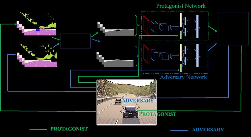
2      P. Gupta et al.

for pedestrians and nearby vehicles and simulate edge cases that may lead to
collisions. From these data, AV’s neural networks learn features and typical re-
sponses but suffer limited (edge) data availability leading to model overfit and
poor generalizability. As a result, operational vehicles exposed to unseen condi-
tions even slight variations on training data may behave unexpectedly, with
grave consequences.
     Simulators generate synthetic data, and augmentation tools increase data
variability. However, simulations rely upon models with inherent biases, simpli-
fications, or omissions. Specifically, traditional simulations implement scenarios
designed by human users or with variational tools, leading to excluded edge cases.
Researchers may utilize randomized scenarios to find edge cases from which to
learn, but entropy is difficult to model. Human behavior, maintenance issues,
and logical errors lead to a range of unpredictable behavior. These simulations
lack the entropy of a chaotic environment which is critical to effectively train a
defensive self-driving car. To this end, we introduce a “Physically Adversarial
Intelligent Network (PAIN),” pitting self-driving cars against one another to cre-
ate a hostile, entropic environment. PAIN is based on “Generative Adversarial
Networks (GANs) [8],” a means of pitting two neural networks, like those used
to pilot self-driving cars [7], against one another to improve driving policies for
both the attacker and the defender.
     In this paper, we pit a protagonist and an adversary agents against one an-
other in the CARLA [5] simulation environment. The protagonist’s objective
is to drive safely from a start to a goal location, while the adversary seeks to
maximize the damage to the protagonist. This helps generate real-world, noisy
data where the protagonist learns to anticipate and avoid impending direct col-
lisions, while the adversary learns to cause increasingly-unpredictable collisions.
The resultant data are better-representative of real-world scenarios than that
provided by pre-programmed or randomized simulation alone.
     Deep Reinforcement Learning (Deep RL) is a popular paradigm to train AV’s
(see [25] for an overview). Algorithms based on deep Q learning [17] and policy
gradient methods [17] may be utilized to train agents with discrete and continu-
ous action spaces, respectively. To ease implementation on constrained compute
platforms, like those found in AVs, we selected the efficient Dueling Double Deep
Q Network (DDDQN) [30] with prioritized experience replay [30] algorithm. We
additionally utilize assisted exploration by incorporating a stochastic PID con-
troller during exploration, and frame-skip [3] to accelerate training. We show
that the protagonist trained with an adversary learns to drive defensively and
exhibits higher success rate (safely reaching the goal location), with an increase
in Mean-Time-to-Failure (MTTF) and average travel distance in unseen driving
scenarios than the agent trained alone. We also show that with no surrounding
vehicles, adversarial training does not impact performance negatively.
     The major contributions of this work are fourfold:
  1. We introduce PAIN, which pit self-driving vehicles with different objectives
      against one another with the environment-in-the-loop.
  2. We utilize the DDDQN algorithm with prioritized experience replay to train
      self-driving agents in a CARLA simulation environment.
Towards Safer Self-Driving Through Great PAIN        3

 3. We utilize assisted exploration and frame-skip to speed up training of the
    coupled agents.
 4. We show that the trained “defensive driving” agent becomes more resilient
    to edge cases than the agent trained without an adversary.
Specifically, we show that the PAIN-trained avoidance algorithm outperforms
the baseline (protagonist trained alone) in all measured performance metrics.
    This manuscript is structured as follows: in Section 2, we discuss prior art.
In Section 3, we formulate the problem, provide input representation and de-
sign reward functions for the two agents. We review Q-learning and traditional
deep-Q learning algorithms in Section 4. We discuss the DDDQN with priori-
tized experience replay, provide network architecture, and explore methods to
accelerate training in Section 5. Simulation scenarios and results are provided in
Section 6, and we conclude in Section 7 by identifying future opportunities and
directions for continued work.

2   Related Work

Deep RL for automated driving: Deep RL has demonstrated remarkable per-
formance in sequential decision making tasks such as computer games [20] and
robotic control [18]. This growing popularity of Deep RL has made it popu-
lar for training AVs. [25] reviews Deep RL approaches for automated driving
and presents a framework leveraging Q-learning [31], Long-Short-Term-Memory
(LSTM) networks [12], and Convolutional Neural Networks (CNN’s) [16]. End-
to-end approaches such as imitation learning [4,23] have shown promising results.
In [3], the authors compare performance of model-free Deep RL algorithms such
as DDQN [29], twin delayed deep deterministic policy gradient (TD3) [6], and
soft actor critic (SAC) [10] for automated urban driving. While the SAC performs
best in urban autonomous driving, policy gradient methods (TD3 and SAC) are
unsuitable for constrained compute platforms. DDDQN is a viable alternative
for constrained platforms and improves upon challenges in traditional deep Q
learning algorithms such as Q-value overestimation and unstable learning.
    Robust Adversarial Reinforcement Learning (RARL): Many RL algorithms
find a single policy that works on simulated data but may not adapt to the real
world. The reality gap [24] while transferring model domains is partly due to
insufficient simulated data and limited scenario coverage leading to untrained
edge cases. [22,24] propose RARL as an extension to RL inspired by robust con-
trol methods. RARL uses two neural networks, a protagonist and an adversary,
pitted against one another in a two player zero-sum game seeking to maximize
and minimize a common reward function, respectively. The adversary acts as a
destabilizing disturbance to the protagonist. In [22], the two agents take turns
performing actions to control the same vehicle so that the protagonist learns
to robustly navigate a simulated race track. In RARL, the learning process in-
volves alternately fixing one agent’s policy while the other agent trains and then
switching until both agents’ policies converge. The trained protagonist learns
to overcome disturbances while the adversary learns to produce more effective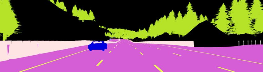
4 P. Gupta et al.
disturbances. Although the two neural networks control the same vehicle, the
action space of the protagonist and the adversary are different. This allows the
designer to model the actions of the adversary to match the expected distur-
bances that are encountered in the physical world. This forces the protagonist
to learn robust policies capable of overcoming the realty gap.
Multi-agent reinforcement learning (MARL): MARL [2, 13] extends RL to
multi-agent systems by combining single-agent RL with game theory. MARL
with competing agents can be viewed as an instance of RARL, where the adver-
sary is an agent competing in the same environment. The adversary’s goal is still
to thwart the protagonist, but as an entity rather than a disturbance. Promising
results have been shown for MARL in [1], where a game of virtual, team-based
hide and seek led to complex behaviors. Like RARL, one team sought to max-
imize its reward, thereby minimizing the opposing team’s reward and forcing
both to learn new strategies to thwart one another. [1] found that the learn-
ing algorithm may find and exploit faults in the simulation environment which
amplifies the reality gap problem.
This approach can help generate data better-representative of the real-world
through the PAIN framework. MARL will force the protagonist to learn robust
policies under uncertainty, while the adversary will find novel strategies to crash,
forcing the inclusion of edge cases in the training data.
3 Problem Formulation
We consider two agents, an adversary and a protagonist, that seek-to-collide and
to avoid collisions, respectively. The agents are trained using model-free Deep
RL in the CARLA simulation environment (an open-source simulator for AV
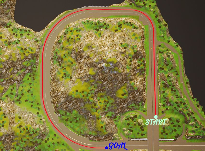
research). Figure 1 shows the protagonist’s 1.4 km desired route. The red curve
Fig. 1: Bird-eye view of the track
shows the trajectory the trained protagonist should learn to drive safely from
the start location (green circle) to the goal location (blue circle). We allow nine
Towards Safer Self-Driving Through Great PAIN 5
discrete actions A ∈ A for both agents, given by:
A = (T, S), where (1)
T ∈ {Constant, Accelerate, Decelerate} and S ∈ {Constant, Steer left, Steer right}.
For each action A = (T, S), the control commands are calculated based on the
previous control input:
Stpr ,
if S = Constant,
St(Stpr , A) = min{Stpr + 0.2, 1}, if S = Steer right, (2a)
max{Stpr − 0.2, −1}, if S = Steer left,
T hpr ,
if T = Constant,
T h(T hpr , A) = min{T hpr + 0.2, 1}, if T = Accelerate, (2b)
max{T hpr − 0.2, 0}, if T = Decelerate,
Brpr ,
if T = Constant,
Br(Brpr , A) = 0, if T = Accelerate, (2c)
max{Brpr + 0.2, 1}, if T = Decelerate,
where St ∈ [−1 1], T h ∈ [0 1], and Br ∈ [0 1] are the steering, throttle and brake
commands with subscript pr denoting the control commands at previous time
step. Incremental, control-targeted changes avoid abrupt changes in the outputs
that might violate a real vehicle’s kinematic constraints. We now provide our
input representation and reward structures for the agents.
3.1 Input Representation
(a) (b)
(c) (d)
Fig. 2: The visible car is an adversary seen by the progatonist’s front view a) RGB front
view, b) Semantic segmentation (CARLA segmented camera view), c) Post-processed,
masked image, d) Normalized gray-scale image used as network input
The CARLA simulation environment includes high-dimensional information
like road markings, traffic signs, objects, and weather effects. While AV’s require
these data for safe operation, the aim of this work is to study the impact of an6 P. Gupta et al.
adversary on training “defensive” agents and therefore does not require taking
traffic laws into consideration. Unlike a real-world AV which would utilize RGB
cameras, LiDAR, RADAR, and other sensors to cover the 360◦ field-of-view of
the vehicle, we instead utilize only the front view image, capturing 110◦ field-of-
view as perceptive input.
To simplify the high-dimensional front view, we utilize CARLA’s semantic
camera to pre-segment an image. Due to recent advances in semantic segmen-
tation [11], AVs can be equipped with such algorithms [9]. We therefore assume
the availability of such data.
We further reduce the state complexity by post-processing the semantically
segmented image to mask out vegetation and road markings. Figures 2a and 2b
show a protagonist’s front-view captured by (a) an RGB camera and (b) the
semantic segmentation camera. The processed, masked image is shown in Fig-
ure 2c. This image is converted to a normalized gray-scale image (Figure 2d) of
size 100x120, which is used in a sequence of four consecutive frames (to predict
vehicle motion) as a perceptive input to the neural network. To simplify motion
computation, we assume the availability of onboard sensors describing vehicle
pose and relative motion. Therefore, our augmented input state s ∈ S to the
neural network consists of:
1. sequence of four segmented, masked, normalized grayscale forward images,
2. vehicle motion state: (vlon , vlat , ω, alon , alat ) and,
3. previous control commands: (T hpr , Stpr , Brpr ),
where, vlon (alon ) and vlat (alat ) represents the longitudinal and lateral velocity
(acceleration) of the ego vehicle, respectively, and w represents its yaw rate. Ve-
hicle motion state and control commands are easily accessible through common
vehicle sensors such as IMU’s, GNSS, encoders, etc.
Figure 3 shows the PAIN framework with the two coupled networks and
the CARLA environment-in-the-loop. By using low-dimensional input data, the
trained algorithm will potentially be suitable for research and development on
low-cost single board computers, eventually enabling PAIN to be trained on
inexpensive physical test platforms [27].
3.2 Reward Design
Protagonist: The protagonist’s objective is to safely drive from a start loca-
tion to a goal location (Figure 1) in the minimum time without any collisions,
subject to a maximum “safe” acceleration limit. This limit ensures the vehicle
stays within the traction limits of the tire and suspension, as well as improves
the occupancy experience for passengers by minimizing large and potentially-
disruptive accelerations. For each state s ∈ S (Section 3.1) and action AP ∈ A
by the protagonist, we design the reward function RP (s, AP ) ∈ R:
RP (s, AP ) = RvP − RaP − Rst
P P
+ Rgoal P
− Rcol P
− Rcross , (3)
where RvP , RaP , Rst
P P
, Rcol P
, Rgoal P
, and Rcross are the rewards based on absolute
velocity v , absolute acceleration a , steering angle stP , collision event, distance
P PTowards Safer Self-Driving Through Great PAIN 7
Fig. 3: System framework with two coupled networks and environment-in-the-loop.
Sequence of processed semantic segmented front view images along with vehicle motion
and control states form a low-dimensional input for each agent, which then uses a deep
neural network to estimate Q values, which help calculate control commands.
to goal disgoal , and cross-track error ePcross (minimum euclidean distance from
protagonist location to its target trajectory), respectively. Reward terms are
defined as following:
−r1 ,
if v P ≤ vmin ,
P P
v
Rv = r2 × vmax (cos(θP ) − sin(θP )), if vmin ≤ v P ≤ vmax , (4)
0, if v P > vmax ,
RaP = r3 × 1(aP >= amax ), (5)
P
Rst = r4 × (stP )2 , (6)
P disgoal
Rgoal = r5 × 1 − + r6 × 1(disgoal < δ), (7)
Routelength
P
Rcol = r7 × 1(collisionP ), (8)
2
2 × eP
P cross
Rcross = r8 × , (9)
roadwidth
where ri , i ∈ {1, · · · , 8} are positive constants, θP is the angle of the protagonist
velocity with respect to the lane, and 1(·) represents the indicator function which
is true when the corresponding condition (·) is true. v P cos(θP ) (-v P sin(θP ))
encourages (penalizes) the velocity of the protagonist along (normal to) the
direction of the lane. vmin , vmax and amax are constants representing minimum
and maximum limits of the absolute velocity and acceleration. The penalty −r1
in RvP minimizes unnecessary stopping. RaP and Rst P
penalizes the agent for large
accelerations and over-steering, respectively, to improve stable and comfortable8 P. Gupta et al.
P
driving. Rcol provides a penalty for collisions determined by the CARLA collision
detector, which provides information such as object ids and intensity for each
P
occurrence. Rgoal provides a reward based on the distance to the goal normalized
against the route length Routelength . It also provides a reward if the protagonist
P
successfully reaches the goal point within a threshold δ. Rcross penalizes the
vehicle based on the cross-track error from the desired path which we normalize
with the half-width of the road road2width .
Other reward functions were considered, including functions that replace RvP
P
and Rgoal with:
−r1 ,
if v P ≤ vmin ,
P P
v
Rv = r2 × vmax , if vmin ≤ v P ≤ vmax , (10)
P
0, if v > vmax ,
P dissubgoal
Rgoal = r5 × 1 − + r6 × 1(disgoal < δ), (11)
disseg
where we divided the protagonist target trajectory into segments of length disseg ,
with each segment end waypoint acting as an intermediate destination. Based
on the segment closest to the protagonist, a reward based on the distance to the
next sub-goal point dissubgoal encouraged it to follow the sub-goals to reach the
final goal location. However, frequent transitions in sub-goal way-points with
changing-segments lead to unstable driving at transition points due to sudden
variation in dissubgoal . Furthermore, this RvP leads to perpetual collisions due to
large velocity component normal to the lane. (4) and (7) performed better as a
reward function.
Adversary: The adversary aims to maximize the peak absolute value of its
acceleration by colliding with the protagonist. Due to limited front perceptive
field of both the agents, we spawn the adversary facing towards the protagonist at
some distance. We design the adversary’s objective function to encourage driving
towards the protagonist (without environmental collisions), making collision with
the protagonist the top priority. For each state s ∈ S and action AA ∈ A by the
adversary, we utilize the reward function Radv (s, AA ) ∈ R:
RA (s, AA ) = RvA + Rcol
A A
+ Rdis A
− Rcross A
+ Rgoal A
− Rst , (12)
where RvA , Rcol
A A
, Rdis A
, and Rcross are rewards based on the absolute velocity v A ,
collision event, distance from the protagonist dispro , and cross-track error eAcross ,
respectively. To encourage driving towards the protagonist, we do online route
planning from the adversary spawn location to the protagonist start point and
A A A
utilize it to compute the cross-track error term Rcross . Rgoal , and Rst rewards
are analogous to the protagonist’s to encourage driving towards the goal point
(starting point of protagonist) and limiting over-steering, respectively. Other
terms are defined as:
(
vA
P r2 × vmax (cos(θA ) − sin(θA )), if 0 ≤ v A ≤ vmax ,
Rv = (13)
0, if v A > vmax ,Towards Safer Self-Driving Through Great PAIN 9
A
Rcol = r10 × 1(collisionA = pro) − r7 × 1(collisionA 6= pro), (14)
A dispro
Rdis = r9 × 1 − , (15)
d
2
2 × eA
A cross
Rcross = r8 × × 1(eAcross > ∆), (16)
roadwidth
where r9 , r10 , ∆ and d are positive constants. RvA provides reward to the ad-
versary for driving at high velocity opposite to the protagonist, since doing so
A
will produce peak maximum acceleration and maximum damage potential. Rcol
provides a reward to the adversary in case of successful collision with the pro-
A
tagonist and penalizes it for colliding with the environment. Rdis rewards the
A
adversary based on its distance to the protagonist. The term Rcross penalizes
the adversary for large (> ∆) cross-track error, making the adversary trajectory
susceptible to environmental collisions. This avoids forcing any specific trajec-
A A
tory on the adversary. Note that without the reward terms Rcross , Rgoal , and
A
Rst , the adversary learns to circle in the roadway at vmax , blocking the protag-
onist’s route. While such a policy will produce high hit rate for the adversary,
the generated data will not be as diverse as that from other policies.
4 Review of Deep Q Learning Algorithms
In RL, Q-learning [32] is often used to train agents with discrete action spaces.
Deep Q-learning algorithms such as Deep Q Networks (DQN) [20] and Double
Deep Q Networks (DDQNs) [29] utilize neural networks to better contend with
large state spaces by estimating Q-values. In this section, we review Q-learning,
followed by a discussion on common deep Q learning algorithms for discrete
action spaces.
Q-Learning: Q-learning is an off-policy model-free RL approach in which the
agent estimates the optimal Q-value for each action. For a given policy π, a
true Q-value (or action-value) for action a, Qπ (s, a), is defined as the expected
discounted reward for executing action a at current state s and following policy
π thereafter. Therefore,
Qπ (s, a) ≡ E[R1 + γR2 + ...|S0 = s, A0 = a, π], (17)
where γ ∈ [0, 1] is a discount factor that represents the trade off between the
importance of immediate and future rewards. The optimal Q-value is defined
∗
as Q∗ (s, a) ≡ Qπ (s, a) = maxπ Qπ (s, a), such that V ∗ (s) = maxa Q∗ (s, a) is
the optimal value in state s. Since an optimal policy is unknown during learning
stage, the objective for any Q-learning based algorithm is to estimate the optimal
Q-values, Q∗ (s, a), from which an optimal policy may be formed as π ∗ (s) ≡ a∗ =
argmaxa Q∗ (s, a). Although there might exist multiple optimal policies π ∗ , the
optimal Q-values are unique.10 P. Gupta et al.
To solve problems with large state-spaces, deep Q-learning methods approxi-
mate Q∗ (s, a) with a parameterized value function Q(s, a; w). These parameters
are updated after taking action At in state St and observing the immediate
reward Rt+1 and resulting state St+1 . This can be expressed as
wt+1 = wt + α(YtQ − Q(St , At ; wt ))∇wt Q(St , At ; wt ) (18)
where α is a step size and YtQ is the target Q-value defined as
YtQ ≡ Rt+1 + γ max Q(St+1 , a; wt ) (19)
a
We now review two commonly used deep Q learning algorithms: DQN’s and
DDQN’s, which utilize neural networks to estimate the optimal Q-values.
Deep Q Network (DQN): DQN utilizes a neural network that takes a state
as an input and approximates the Q-values for each discrete action based on
that state. The network weights are updated using stochastic gradient descent
resembling (18) and (19). The original DQN algorithm suffers from drawbacks
including slow convergence and unstable learning as the target Q-values change
in conjunction with the weight updates. It also suffers from over-estimation of
the Q-values due to lack of information about the Q-function in initial training
stages. Choosing actions by maximizing potentially poorly-estimated Q-values in
these stages can lead to sub-optimal policies. DQN algorithm discards experi-
ences after a single update, failing to learn from possibly rare and useful expe-
riences. The streaming experiences make the updates strongly correlated which
violates the i.i.d. assumption of many stochastic gradient-based algorithms.
Two advances using target networks and experience replay have been pro-
posed [21] to improve the performance of the DQN algorithm. First, a target
network Q(s, a; w− ), with parameters w− , is used to update the target Q-values
YtDQN used by DQN by modifying (19) to
YtDQN ≡ Rt+1 + γ max Q(St+1 , a; wt− ). (20)
a
Target network weights w− are copied from the online network weights w
every τ steps, and kept fixed during other steps. This speeds convergence during
training as well as provides a more stable learning process. The second advance
utilizes experience replay, in which past experiences are stored in a memory for a
time and this memory is sampled uniformly to update the network. This makes
weight updates less correlated and reuses past experiences to enhance training.
Double Deep Q Network (DDQN): Double Deep Q-Networks [29] improve
upon the DQN algorithm by decoupling action selection from action evaluation,
thereby reducing the likelihood of overestimation of Q-values. The update equa-
tion for DDQN weights is the same as that for DQN, with the exception that
the target value YtDQN is replaced by YtDDQN , defined as:
YtDDQN ≡ Rt+1 + γQ(St+1 , argmax Q(St+1 , a; wt ), wt− ) (21)
aTowards Safer Self-Driving Through Great PAIN 11
where wt− are the weights of the target network from the DQN.
Although DDQN improves upon DQN, both methods fails to identify the
difference between desirable and undesirable states, and suffer from overesti-
mation of Q values and unstable learning. An automated vehicle trained with
these algorithms might learn an unstable sub-optimal policy resulting in frequent
failures including collisions. A Dueling, Double Deep Q Network (DDDQN) [30]
improves upon these by estimating Q-values in a more reliable, faster, and stable
manner. We illustrate this further in Section 5.
5 Physically Adversarial Intelligent Network
The PAIN framework trains coupled networks in a high-entropy environment
to learn robust protagonist and adversary policies. We utilize DDDQN with
prioritized experience replay for agent training. We now discuss the PAIN im-
plementation’s algorithms, architecture, and methods.
5.1 Dueling Double Deep Q Network (DDDQN)
In some states, the next action is critical. In others, it makes little difference.
Whereas a action state may be critical for safety when driving on a narrow curvy
road, it may not be in a wide open parking lot. For states with minimal action
impact, it is unnecessary to estimate each action’s value. To this end, DDDQN
estimates Q-values by aggregating the state value V (s) of being at a state and
the advantage A(s, a) of taking a specific action at that state. This is realized
by splitting the output of the convolutional layers in a deep-Q network into two
streams of fully connected layers, one for estimating value of the state V (s) and
the other for the action advantage A(s, a). The final Q-value estimate in DDDQN
is obtained by aggregating estimates in an aggregation layer as following:
1
Q(s, a; w, α, β) = V (s; w, β) + (A(s, a; w, α) − A(s, a0 ; w, α)), (22)
|A|
where w, α, β are the common network weights, advantage stream parameters,
and the value stream parameters, respectively. Decoupling into two streams ac-
celerates training by providing a more reliable estimate of Q values for each
action [30]. Additionally, the network learns to identify whether a state is de-
sirable while identifying the importance of each actions in that state. DDDQN
therefore allows for faster, stable learning with reliable Q-value estimates.
5.2 Prioritized Experience Replay (PER)
PER [26] is an algorithm for sampling a batch of experiences from a memory
buffer to train a network. It improves the policy learned by DQN algorithms by
increasing the replay probability of experiences that have a high impact on the
learning process. These experiences may be rare but informative. The prediction12 P. Gupta et al.
error of the Q-learning algorithm is used to assign a priority value pi for each
experience stored in a memory buffer, which then generates a probability
pλ
P(i) = P i λ (23)
k pk
by normalizing the priority values pi with the total priority values of all the
experiences held in the memory. λ ∈ [0, 1] is a hyper-parameter that adds
randomness to experience selection. Sampling experiences from memory based
on (23) tends to add bias to the training data since high priority experiences
will get selected more often. To remove this bias, PER weights experiences with
importance sampling weights (IS) calculated as
1 1 µ
ωi = , (24)
N P(i)
where N is the number of experiences in memory, and the hyper-parameter
µ ∈ [0, 1] controls the impact of IS weights on learning. The hyper-parameter µ
is typically increased from a small value to 1 throughout training because the
weights are most important late in training (when Q-values start to converge).
PER improves learning speed and policy quality when compared to uniform
experience replay [26].
5.3 Network Architecture
Fig. 4: Neural Network architecture for both the agents.
Figure 4 shows our DDDQN-based neural network architecture for both the
agents. The sequence of four stacked normalized gray-scale images of size 100x120
is passed through 3 convolution layers with filter sizes 8x8x4-s-4, 4x4x32-s-2, and
4x4x64-s-2. The output after 3 convolutions (4x5x128) is flattened and passed
to two 512-dimensional fully connected layers along with the vehicle motion
state and previous control commands (see Section 3.1). The two fully connectedTowards Safer Self-Driving Through Great PAIN 13
layers estimate a one dimensional state value V (s) and 9 dimensional advantage
vector A(s, ai ), i ∈ {1, 2, · · · , 9}. Finally, the state value and advantage vector are
aggregated ((22)) through an aggregation layer to produce a 9-dimensional vector
corresponding to the Q-values for all possible actions. Similar architectures have
been used to train agents to play computer games [28].
5.4 Assisted Exploration
Algorithm 1 Assisted Exploration using PID controller
Input: Set of all actions A, PID action=AP ID ∈ A, Exploration probability , state
s, DDDQN network N et, Previous Control command (Stpr , T hpr , Brpr )
Output: Action A and Control command (St, T h, Br)
1: procedure GETACTION
2: Sample a random number α ∈ [0 1]
3: if α < then
4: PID probability PP ID ← 0.75
5: Sample a random number αP ID ∈ [0 1]
6: if αP ID < PP ID then
7: Action A ← AP ID
8: else
9: Sample a random action A ∈ A
10: else
11: Obtain network estimated Q values Q ← N et(s)
12: Action A ← argmaxa∈A {Q}
13: (St, T h, Br) ← CON T ROL((Stpr , T hpr , Brpr ), A)
14: return A, (St, T h, Br)
Due to high-dimensional state space for autonomous driving, training is time-
intensive. Researchers utilize techniques like imitation and transfer learning to
speed up the training process [27]. We introduce assisted exploration utilizing a
stochastic PID controller during exploration to speed up the training process.
Specifically, we tune a PID controller to follow a target path and utilize it to
generate preconditioning data along with the random exploration during train-
ing. Unlike the epsilon greedy approach, where random action are chosen during
exploration, we choose exploration actions based on PID controller with proba-
bility PP ID and random actions with probability 1 − PP ID . The probability of
sampling action from PID controller PP ID is decreased with training steps to
reduce the effect of PID controller over time. Algorithm 1 provides pseudo-code
for the assisted exploration strategy. The input exploration probability expo-
nentially decreases from its maximum max to min at a decay rate of ∆ with
training steps tsteps :
= min + (max − min ) ∗ exp(−∆ ∗ tsteps ), (25)
where min = 0.01, max = 1, and ∆ = 0.000001. Since the output of the
PID controller does not necessarily satisfy (2), the input PID action AP ID ∈ A14 P. Gupta et al.
is calculated by mapping the output of PID controller and previous control
command to the corresponding action in A. Without assisted exploration, the
untrained agent may not explore enough of the state space to learn an effective
policy from random actions.
The function CON T ROL((Stpr , T hpr , Brpr ), A) calculates the control in-
put using (2).
5.5 Frame skip
We utilize frame-skip technique to further accelerate training. In frame-skip, the
action of the agent is kept unchanged for k consecutive frames, after which a
new action is applied for next k. This technique reduces training complexity
and leads to stable policies. While training the protagonist, we change k from
one to three at pre-determined intervals. Initially actions are chosen from the
PID controller with high probability. Utilizing frame skip and PID with large
k causes error accumulation and unstable agent motion, and frame-skip with
random actions also leads to frequent collisions. Therefore, we increase k from
one to three after significant reduction in the exploration probability.
6 Experimental Evaluation
6.1 Training and simulation scenario
We first train the protagonist alone to learn a policy to reach the goal location
without collisions. This model serves as a baseline for the protagonist. Once the
baseline model learns to safety drive the route, we start our coupled training
with the adversary. We clone the baseline policy to use as the initial policy for
both the adversary and protagonist. We train two models for the protagonist;
Model 1 (243K episodes) and Model 2 (353K episodes).
6.2 Performance Evaluation
We utilize success rate, mean-time-to-failure (MTTF) and mean distance trav-
eled (normalized with total route length) as performance metrics for the pro-
tagonist. The success rates are recorded at four checkpoints: 25%, 50%, 75%,
and 95% of route length. If the protagonist successfully reaches the goal point,
the MTTF corresponds to its track completion time. In case of failure through
collision, we record the event’s collision intensity (CI).
We evaluate the protagonist’s performance in four scenarios: (1) without any
surrounding vehicles; (2) with 50 nearby vehicles driving in CARLA autopilot
mode; (3) 5 static vehicles obstructing the protagonist’s route; and (4) against
the adversary. Any vehicle initialized in autopilot mode randomly drives around
the environment while respecting driving rules. We conduct 100 trials for each
scenario and compare the performance with the baseline model of the protagonist
trained without an adversary.Towards Safer Self-Driving Through Great PAIN 15
Scenario 1: No surrounding vehicles
We evaluate the performance of the protagonist in an environment with no
other vehicles. This is the baseline agent’s training environment, a useful sce-
nario to evaluate whether the PAIN degraded baseline performance in safe en-
vironments (e.g. by learning over-conservative policies such as slow driving, or a
bangbang control strategy).
All tested models were able to complete the track with a 100% success rate
and therefore traveled the same distance without any collisions. The average
reward of all the models were similar which indicates that the performance of
the PAIN’s protagonist does not deteriorate in safe environments.
Scenario 2: Dynamic vehicles in autopilot mode
This scenario emulates typical driving with surrounding vehicles. We ran-
domly spawn 50 vehicles driving in autopilot mode in the environment. Due to
the large environment, the agent might only interact with few vehicles (5-15)
along its route. This scenario is a challenging as the protagonist has never seen
more than one vehicle (the adversary) during training.
Some rear-end collisions occurred, which is unavoidable due to limited per-
ceptive field (110◦ field-of-view) for all models’ input. Table 1 compares the per-
formance of the protagonist in Scenario 2 with the baseline model. Protagonists
trained through PAIN framework outperform the baseline in all performance
metrics, and Model 2 outperforms Model 1 in all metrics, indicating that the
PAIN framework will continue to improve over long timescales.
Model Model 1 Model 2 Model Baseline Model 1 Model 2
Average Reward 89.0% 107.6% 25% Route 73% 86% 90%
MTTF 38.0% 44.9% 50% Route 58% 77% 87%
Average Distance 29.6% 41.8% 75% Route 40% 65% 77%
Average CI -44.5% -65.5% 95% Route 23% 49% 61%
Table 1: Protagonist performance in Scenario 2. (Left table) Percentage change from
the baseline model, (Right table) Success Rate
Scenario 3: Static vehicles obstructing the protagonist route
In this scenario, we obstruct the protagonist’s trajectory by spawning 5 static
vehicles along its route. We choose random spawn locations for static vehicles
from the waypoints encountered by the protagonist in absence of surrounding
vehicles. This provides edge cases where the static vehicles block the road and
emulate real world accidents, roadkill, etc. It is a challenging scenario for the
protagonist because: (i) multiple vehicles were not encountered in training, (ii)
static vehicles were not in the training set, and (iii) the route blockage created
by static vehicles forces the agent to deviate from its typical trajectory and
attempt high-risk trajectories leading to unseen forwrad-facing camera data.
Table 2 compares the performance of the protagonist models in Scenario 3 with
the baseline model. The protagonist models trained through PAIN framework
outperforms the baseline in all performance metrics.16 P. Gupta et al.
Model Model 1 Model 2 Model Baseline Model 1 Model 2
Average Reward 151.1% 259.3% 25% Route 61% 79% 89%
MTTF 37.0% 63.0% 50% Route 20% 37% 59%
Average Distance 31.9% 64.1% 75% Route 07% 22% 35%
Average CI -15.3% -27.9% 95% Route 04% 12% 22%
Table 2: Protagonist performance in Scenario 3. (Left table) Percentage change from
the baseline model, (Right table) Success Rate
Scenario 4: Against Adversary
This scenario pits the protagonist against a trained adversary. The adversary
was spawned facing towards the protagonist at some random distance in front
of it. We evaluate the hit rate of the adversary, characterized as a successful
adversary-protagonist collision of any force. In 100 trials, the hit rate of the
adversary against the baseline, Model 1 and Model 2 was found to be 22%, 34%,
and 28%, respectively. Since the adversary is trained against the protagonist, it
has a higher hit-rate against these models than the baseline suggesting that, like
the protagonist, the adversary improves over episodes. In practice, we assume
that vehicle collisions are incidental, and therefore the protagonist will be better-
off in day-to-day driving, no matter how effective the adversary becomes.
7 Conclusions and Future Directions
In this work, we proposed a “physically adversarial intelligent network (PAIN)”
pitting multiple AVs against one another with the environment-in-the-loop. The
coupled networks attempt to find faults in one another which improves the per-
formance of both the protagonist and the adversary. We show that the pro-
tagonist trained with the adversary outperforms the baseline model in all per-
formance metrics. The presence of the adversary leads to more robust obstacle
avoidance policies for the protagonist as well as provides edge case training sce-
narios that are difficult to pre-program.
There are several avenues for future research. We plan to extend our dis-
crete action space to a continuous action space, utilizing state-of-the-art policy
gradient methods such as soft actor critic (SAC), and twin delayed deep deter-
ministic policy gradient (TD3). A continuous action space is a natural choice for
the self-driving vehicles, and policy gradient algorithms such as SAC, and TD3
have been successfully used in automated driving [3].
In our future work, we plan to add views from multiple cameras and other
sensors to improve the perceptive field, utilizing transfer learning based on our
current network trained with limited perceptive field to accelerate learning.
Perhaps most important is the planned deployment of a PAIN on small-
scale physical vehicles [27]. It is of interest to transition these trained models
from a simulation environment to scale-model vehicles in order to capture data
stemming from the entropy inherent in physical systems that is difficult to model
in simulations, even those based on the PAIN framework. Hundreds of small-scale
vehicles can be built for the price of one full sized AV, leading to a happy balanceTowards Safer Self-Driving Through Great PAIN 17
of data collection cost, diversity, and speed. Using a physical platform will help
cross the “reality gap” faster and more effectively than is feasible today.
8 Acknowledgements
We thank the NVIDIA Corporation for providing a Titan Xp and Vaibhav Sri-
vastava for providing additional resources supporting this research.
References
1. Baker, B., Kanitscheider, I., Markov, T., Wu, Y., Powell, G., McGrew, B.,
Mordatch, I.: Emergent tool use from multi-agent autocurricula. arXiv preprint
arXiv:1909.07528 (2019)
2. Bu, L., Babu, R., De Schutter, B., et al.: A comprehensive survey of multiagent
reinforcement learning. IEEE Transactions on Systems, Man, and Cybernetics,
Part C (Applications and Reviews) 38(2), 156–172 (2008)
3. Chen, J., Yuan, B., Tomizuka, M.: Model-free deep reinforcement learning for
urban autonomous driving. arXiv preprint arXiv:1904.09503 (2019)
4. Codevilla, F., Miiller, M., López, A., Koltun, V., Dosovitskiy, A.: End-to-end driv-
ing via conditional imitation learning. In: 2018 IEEE International Conference on
Robotics and Automation (ICRA). pp. 1–9. IEEE (2018)
5. Dosovitskiy, A., Ros, G., Codevilla, F., Lopez, A., Koltun, V.: CARLA: An open
urban driving simulator. In: Proceedings of the 1st Annual Conference on Robot
Learning. pp. 1–16 (2017)
6. Fujimoto, S., van Hoof, H., Meger, D.: Addressing function approximation error in
actor-critic methods. arXiv preprint arXiv:1802.09477 (2018)
7. Ghosh, A., Bhattacharya, B., Chowdhury, S.B.R.: Sad-gan: Synthetic autonomous
driving using generative adversarial networks. arXiv preprint arXiv:1611.08788
(2016)
8. Goodfellow, I., Pouget-Abadie, J., Mirza, M., Xu, B., Warde-Farley, D., Ozair,
S., Courville, A., Bengio, Y.: Generative adversarial nets. In: Advances in neural
information processing systems. pp. 2672–2680 (2014)
9. Ha, Q., Watanabe, K., Karasawa, T., Ushiku, Y., Harada, T.: Mfnet: Towards real-
time semantic segmentation for autonomous vehicles with multi-spectral scenes.
In: 2017 IEEE/RSJ International Conference on Intelligent Robots and Systems
(IROS). pp. 5108–5115. IEEE (2017)
10. Haarnoja, T., Zhou, A., Abbeel, P., Levine, S.: Soft actor-critic: Off-policy maxi-
mum entropy deep reinforcement learning with a stochastic actor. arXiv preprint
arXiv:1801.01290 (2018)
11. He, K., Gkioxari, G., Dollár, P., Girshick, R.: Mask r-cnn. In: Proceedings of the
IEEE international conference on computer vision. pp. 2961–2969 (2017)
12. Hochreiter, S., Schmidhuber, J.: Long short-term memory. Neural computation
9(8), 1735–1780 (1997)
13. Hu, J., Wellman, M.P., et al.: Multiagent reinforcement learning: theoretical frame-
work and an algorithm. In: ICML. vol. 98, pp. 242–250. Citeseer (1998)
14. Kahn, G., Villaflor, A., Pong, V., Abbeel, P., Levine, S.: Uncertainty-aware rein-
forcement learning for collision avoidance. arXiv preprint arXiv:1702.01182 (2017)18 P. Gupta et al.
15. Kaur, K., Rampersad, G.: Trust in driverless cars: Investigating key factors in-
fluencing the adoption of driverless cars. Journal of Engineering and Technology
Management 48, 87–96 (2018)
16. Krizhevsky, A., Sutskever, I., Hinton, G.E.: Imagenet classification with deep con-
volutional neural networks. In: Advances in neural information processing systems.
pp. 1097–1105 (2012)
17. Li, Y.: Deep reinforcement learning: An overview. arXiv preprint arXiv:1701.07274
(2017)
18. Lillicrap, T.P., Hunt, J.J., Pritzel, A., Heess, N., Erez, T., Tassa, Y., Silver, D.,
Wierstra, D.: Continuous control with deep reinforcement learning. arXiv preprint
arXiv:1509.02971 (2015)
19. Madrigal, A.C.: Inside waymos secret world for training self-driving cars. The At-
lantic 23 (2017)
20. Mnih, V., Kavukcuoglu, K., Silver, D., Graves, A., Antonoglou, I., Wierstra, D.,
Riedmiller, M.: Playing atari with deep reinforcement learning. arXiv preprint
arXiv:1312.5602 (2013)
21. Mnih, V., Kavukcuoglu, K., Silver, D., Rusu, A.A., Veness, J., Bellemare, M.G.,
Graves, A., Riedmiller, M., Fidjeland, A.K., Ostrovski, G., et al.: Human-level
control through deep reinforcement learning. Nature 518(7540), 529 (2015)
22. Pan, X., Seita, D., Gao, Y., Canny, J.: Risk averse robust adversarial reinforcement
learning. arXiv preprint arXiv:1904.00511 (2019)
23. Pan, Y., Cheng, C.A., Saigol, K., Lee, K., Yan, X., Theodorou, E., Boots, B.: Agile
autonomous driving using end-to-end deep imitation learning. In: Robotics: science
and systems (2018)
24. Pinto, L., Davidson, J., Sukthankar, R., Gupta, A.: Robust adversarial reinforce-
ment learning. In: Proceedings of the 34th International Conference on Machine
Learning-Volume 70. pp. 2817–2826. JMLR. org (2017)
25. Sallab, A.E., Abdou, M., Perot, E., Yogamani, S.: Deep reinforcement learning
framework for autonomous driving. Electronic Imaging 2017(19), 70–76 (2017)
26. Schaul, T., Quan, J., Antonoglou, I., Silver, D.: Prioritized experience replay. arXiv
preprint arXiv:1511.05952 (2015)
27. Siegel, J.E., Pappas, G., Politopoulos, K., Sun, Y.: A gamified simulator and phys-
ical platform for self-driving algorithm training and validation (2019)
28. Simonini, T.: A free course in deep reinforcement learning from begin-
ner to expert (2018), http://simoninithomas.github.io/Deep_reinforcement_
learning_Course/
29. Van Hasselt, H., Guez, A., Silver, D.: Deep reinforcement learning with double
q-learning. In: Thirtieth AAAI conference on artificial intelligence (2016)
30. Wang, Z., Schaul, T., Hessel, M., Van Hasselt, H., Lanctot, M., De Freitas, N.:
Dueling network architectures for deep reinforcement learning. arXiv preprint
arXiv:1511.06581 (2015)
31. Watkins, C.J., Dayan, P.: Q-learning. Machine learning 8(3-4), 279–292 (1992)
32. Watkins, C.J.C.H.: Learning from delayed rewards (1989)You can also read