PointRend: Image Segmentation as Rendering
←
→
Page content transcription
If your browser does not render page correctly, please read the page content below
PointRend: Image Segmentation as Rendering

                                                                 Alexander Kirillov         Yuxin Wu          Kaiming He            Ross Girshick
                                                                                      Facebook AI Research (FAIR)

                                                                                                                       Mask R-CNN                         + PointRend
                                                                  Abstract
arXiv:1912.08193v2 [cs.CV] 16 Feb 2020

                                            We present a new method for efficient high-quality
                                         image segmentation of objects and scenes. By analogizing
                                         classical computer graphics methods for efficient rendering
                                         with over- and undersampling challenges faced in pixel
                                         labeling tasks, we develop a unique perspective of image                                       28×28                           224×224
                                         segmentation as a rendering problem. From this vantage,
                                         we present the PointRend (Point-based Rendering) neural
                                         network module: a module that performs point-based
                                         segmentation predictions at adaptively selected locations
                                         based on an iterative subdivision algorithm. PointRend
                                         can be flexibly applied to both instance and semantic                    28×28             56×56           112×112          224×224
                                         segmentation tasks by building on top of existing state-of-
                                                                                                              Figure 1: Instance segmentation with PointRend. We introduce
                                         the-art models. While many concrete implementations of               the PointRend (Point-based Rendering) module that makes predic-
                                         the general idea are possible, we show that a simple design          tions at adaptively sampled points on the image using a new point-
                                         already achieves excellent results. Qualitatively, PointRend         based feature representation (see Fig. 3). PointRend is general and
                                         outputs crisp object boundaries in regions that are over-            can be flexibly integrated into existing semantic and instance seg-
                                         smoothed by previous methods. Quantitatively, PointRend              mentation systems. When used to replace Mask R-CNN’s default
                                         yields significant gains on COCO and Cityscapes, for both            mask head [19] (top-left), PointRend yields significantly more de-
                                         instance and semantic segmentation. PointRend’s efficiency           tailed results (top-right). (bottom) During inference, PointRend it-
                                         enables output resolutions that are otherwise impractical            erative computes its prediction. Each step applies bilinear upsam-
                                         in terms of memory or computation compared to existing               pling in smooth regions and makes higher resolution predictions
                                         approaches. Code has been made available at https://                 at a small number of adaptively selected points that are likely to
                                                                                                              lie on object boundaries (black points). All figures in the paper are
                                         github.com/facebookresearch/detectron2/
                                                                                                              best viewed digitally with zoom. Image source: [41].
                                         tree/master/projects/PointRend.

                                                                                                              ally ideal for image segmentation. The label maps pre-
                                         1. Introduction
                                                                                                              dicted by these networks should be mostly smooth, i.e.,
                                            Image segmentation tasks involve mapping pixels sam-              neighboring pixels often take the same label, because high-
                                         pled on a regular grid to a label map, or a set of label maps,       frequency regions are restricted to the sparse boundaries be-
                                         on the same grid. For semantic segmentation, the label map           tween objects. A regular grid will unnecessarily oversample
                                         indicates the predicted category at each pixel. In the case of       the smooth areas while simultaneously undersampling ob-
                                         instance segmentation, a binary foreground vs. background            ject boundaries. The result is excess computation in smooth
                                         map is predicted for each detected object. The modern tools          regions and blurry contours (Fig. 1, upper-left). Image seg-
                                         of choice for these tasks are built on convolutional neural          mentation methods often predict labels on a low-resolution
                                         networks (CNNs) [27, 26].                                            regular grid, e.g., 1/8-th of the input [35] for semantic seg-
                                            CNNs for image segmentation typically operate on reg-             mentation, or 28×28 [19] for instance segmentation, as a
                                         ular grids: the input image is a regular grid of pixels, their       compromise between undersampling and oversampling.
                                         hidden representations are feature vectors on a regular grid,           Analogous sampling issues have been studied for
                                         and their outputs are label maps on a regular grid. Regu-            decades in computer graphics. For example, a renderer
                                         lar grids are convenient, but not necessarily computation-           maps a model (e.g., a 3D mesh) to a rasterized image, i.e. a

                                                                                                          1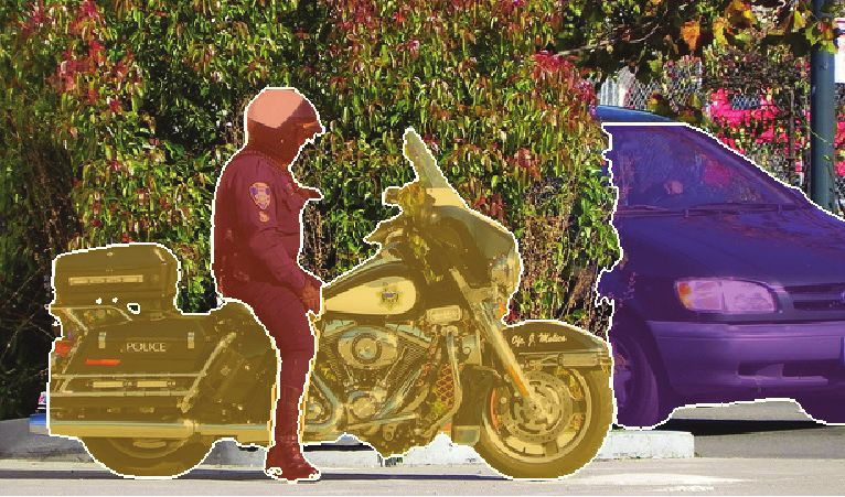
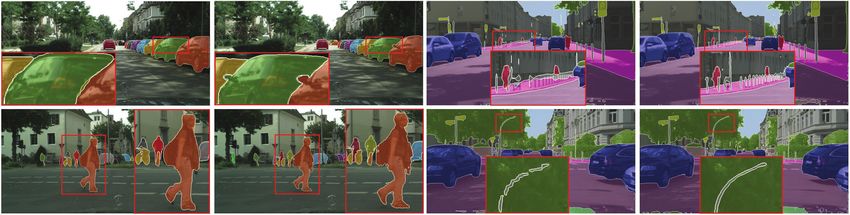
Figure 2: Example result pairs from Mask R-CNN [19] with its standard mask head (left image) vs. with PointRend (right image),
using ResNet-50 [20] with FPN [28]. Note how PointRend predicts masks with substantially finer detail around object boundaries.

regular grid of pixels. While the output is on a regular grid,         output grid, PointRend makes predictions only on carefully
computation is not allocated uniformly over the grid. In-              selected points. To make these predictions, it extracts a
stead, a common graphics strategy is to compute pixel val-             point-wise feature representation for the selected points by
ues at an irregular subset of adaptively selected points in the        interpolating f , and uses a small point head subnetwork to
image plane. The classical subdivision technique of [48], as           predict output labels from the point-wise features. We will
an example, yields a quadtree-like sampling pattern that ef-           present a simple and effective PointRend implementation.
ficiently renders an anti-aliased, high-resolution image.                 We evaluate PointRend on instance and semantic seg-
   The central idea of this paper is to view image seg-                mentation tasks using the COCO [29] and Cityscapes [9]
mentation as a rendering problem and to adapt classical                benchmarks. Qualitatively, PointRend efficiently computes
ideas from computer graphics to efficiently “render” high-             sharp boundaries between objects, as illustrated in Fig. 2
quality label maps (see Fig. 1, bottom-left). We encap-                and Fig. 8. We also observe quantitative improvements even
sulate this computational idea in a new neural network                 though the standard intersection-over-union based metrics
module, called PointRend, that uses a subdivision strategy             for these tasks (mask AP and mIoU) are biased towards
to adaptively select a non-uniform set of points at which              object-interior pixels and are relatively insensitive to bound-
to compute labels. PointRend can be incorporated into                  ary improvements. PointRend improves strong Mask R-
popular meta-architectures for both instance segmentation              CNN and DeepLabV3 [5] models by a significant margin.
(e.g., Mask R-CNN [19]) and semantic segmentation (e.g.,
FCN [35]). Its subdivision strategy efficiently computes               2. Related Work
high-resolution segmentation maps using an order of mag-               Rendering algorithms in computer graphics output a reg-
nitude fewer floating-point operations than direct, dense              ular grid of pixels. However, they usually compute these
computation.                                                           pixel values over a non-uniform set of points. Efficient pro-
   PointRend is a general module that admits many pos-                 cedures like subdivision [48] and adaptive sampling [38, 42]
sible implementations. Viewed abstractly, a PointRend                  refine a coarse rasterization in areas where pixel values
module accepts one or more typical CNN feature maps                    have larger variance. Ray-tracing renderers often use over-
f (xi , yi ) that are defined over regular grids, and outputs          sampling [50], a technique that samples some points more
high-resolution predictions p(x0i , yi0 ) over a finer grid. In-       densely than the output grid to avoid aliasing effects. Here,
stead of making excessive predictions over all points on the           we apply classical subdivision to image segmentation.

                                                                   2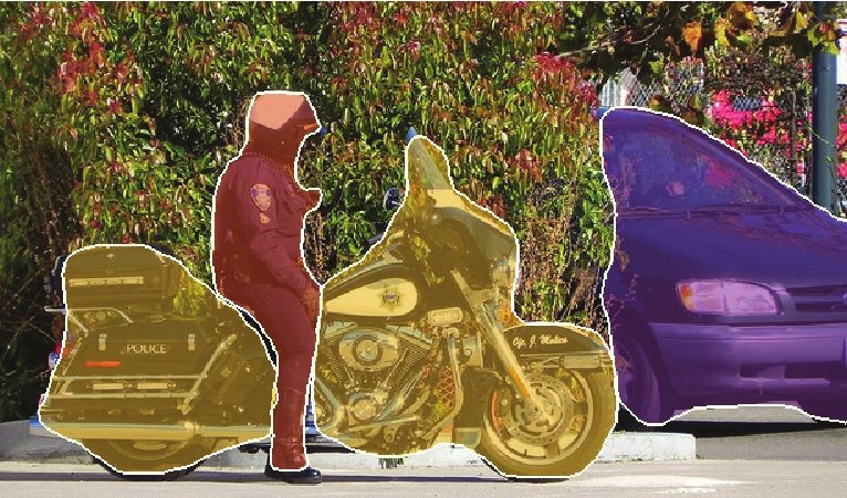
Non-uniform grid representations. Computation on reg-                                                       coarse prediction
ular grids is the dominant paradigm for 2D image analy-
                                                                                       CNN backbone
sis, but this is not the case for other vision tasks. In 3D
shape recognition, large 3D grids are infeasible due to cu-
bic scaling. Most CNN-based approaches do not go be-
yond coarse 64×64×64 grids [12, 8]. Instead, recent works
consider more efficient non-uniform representations such as
meshes [47, 14], signed distance functions [37], and oc-                                                                 MLP
trees [46]. Similar to a signed distance function, PointRend
can compute segmentation values at any point.
    Recently, Marin et al. [36] propose an efficient semantic
                                                                                           fine-grained     point features point predictions
segmentation network based on non-uniform subsampling
                                                                                              features
of the input image prior to processing with a standard se-
mantic segmentation network. PointRend, in contrast, fo-               Figure 3: PointRend applied to instance segmentation. A stan-
cuses on non-uniform sampling at the output. It may be                 dard network for instance segmentation (solid red arrows) takes
possible to combine the two approaches, though [36] is cur-            an input image and yields a coarse (e.g. 7×7) mask prediction for
rently unproven for instance segmentation.                             each detected object (red box) using a lightweight segmentation
                                                                       head. To refine the coarse mask, PointRend selects a set of points
Instance segmentation methods based on the Mask R-                     (red dots) and makes prediction for each point independently with
CNN meta-architecture [19] occupy top ranks in recent                  a small MLP. The MLP uses interpolated features computed at
challenges [32, 3]. These region-based architectures typ-              these points (dashed red arrows) from (1) a fine-grained feature
                                                                       map of the backbone CNN and (2) from the coarse prediction
ically predict masks on a 28×28 grid irrespective of ob-
                                                                       mask. The coarse mask features enable the MLP to make differ-
ject size. This is sufficient for small objects, but for large         ent predictions at a single point that is contained by two or more
objects it produces undesirable “blobby” output that over-             boxes. The proposed subdivision mask rendering algorithm (see
smooths the fine-level details of large objects (see Fig. 1,           Fig. 4 and §3.1) applies this process iteratively to refine uncertain
top-left). Alternative, bottom-up approaches group pixels              regions of the predicted mask.
to form object masks [31, 1, 25]. These methods can pro-
duce more detailed output, however, they lag behind region-
based approaches on most instance segmentation bench-                  3. Method
marks [29, 9, 40]. TensorMask [7], an alternative sliding-
window method, uses a sophisticated network design to                      We analogize image segmentation (of objects and/or
predict sharp high-resolution masks for large objects, but             scenes) in computer vision to image rendering in computer
its accuracy also lags slightly behind. In this paper, we              graphics. Rendering is about displaying a model (e.g., a
show that a region-based segmentation model equipped                   3D mesh) as a regular grid of pixels, i.e., an image. While
with PointRend can produce masks with fine-level details               the output representation is a regular grid, the underlying
while improving the accuracy of region-based approaches.               physical entity (e.g., the 3D model) is continuous and its
                                                                       physical occupancy and other attributes can be queried at
Semantic segmentation. Fully convolutional networks                    any real-value point on the image plane using physical and
(FCNs) [35] are the foundation of modern semantic seg-                 geometric reasoning, such as ray-tracing.
mentation approaches. They often predict outputs that have                 Analogously, in computer vision, we can think of an im-
lower resolution than the input grid and use bilinear upsam-           age segmentation as the occupancy map of an underlying
pling to recover the remaining 8-16× resolution. Results               continuous entity, and the segmentation output, which is a
may be improved with dilated/atrous convolutions that re-              regular grid of predicted labels, is “rendered” from it. The
place some subsampling layers [4, 5] at the expense of more            entity is encoded in the network’s feature maps and can be
memory and computation.                                                accessed at any point by interpolation. A parameterized
   Alternative approaches include encoder-decoder achitec-             function, that is trained to predict occupancy from these in-
tures [6, 24, 44, 45] that subsample the grid representation           terpolated point-wise feature representations, is the coun-
in the encoder and then upsample it in the decoder, using              terpart to physical and geometric reasoning.
skip connections [44] to recover filtered details. Current                 Based on this analogy, we propose PointRend (Point-
approaches combine dilated convolutions with an encoder-               based Rendering) as a methodology for image segmenta-
decoder structure [6, 30] to produce output on a 4× sparser            tion using point representations. A PointRend module ac-
grid than the input grid before applying bilinear interpola-           cepts one or more typical CNN feature maps of C chan-
tion. In our work, we propose a method that can efficiently            nels f ∈ RC×H×W , each defined over a regular grid (that
predict fine-level details on a grid as dense as the input grid.       is typically 4× to 16× coarser than the image grid), and

                                                                   3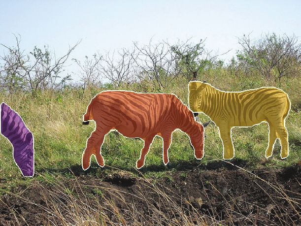
0    0             4×4                               8×8                         8×8
outputs predictions for the K class labels p ∈ RK×H ×W
over a regular grid of different (and likely higher) resolu-                                                               point
tion. A PointRend module consists of three main compo-                                         2×                        prediction
nents: (i) A point selection strategy chooses a small number
of real-value points to make predictions on, avoiding exces-
sive computation for all pixels in the high-resolution output
grid. (ii) For each selected point, a point-wise feature rep-          Figure 4: Example of one adaptive subdivision step. A predic-
resentation is extracted. Features for a real-value point are          tion on a 4×4 grid is upsampled by 2× using bilinear interpola-
computed by bilinear interpolation of f , using the point’s 4          tion. Then, PointRend makes prediction for the N most ambigu-
nearest neighbors that are on the regular grid of f . As a re-         ous points (black dots) to recover detail on the finer grid. This
sult, it is able to utilize sub-pixel information encoded in the       process is repeated until the desired grid resolution is achieved.
channel dimension of f to predict a segmentation that has
higher resolution than f . (iii) A point head: a small neu-                                   k = 1, β = 0.0     k = 3, β = 0.75      k = 10, β = 0.75

ral network trained to predict a label from this point-wise
feature representation, independently for each point.
    The PointRend architecture can be applied to instance
segmentation (e.g., on Mask R-CNN [19]) and semantic
segmentation (e.g., on FCNs [35]) tasks. For instance seg-
mentation, PointRend is applied to each region. It com-                 a) regular grid        b) uniform       c) mildly biased d) heavily biased

putes masks in a coarse-to-fine fashion by making predic-              Figure 5: Point sampling during training. We show N =142
tions over a set of selected points (see Fig. 3). For seman-           points sampled using different strategies for the same underlying
tic segmentation, the whole image can be considered as a               coarse prediction. To achieve high performance only a small num-
single region, and thus without loss of generality we will             ber of points are sampled per region with a mildly biased sampling
describe PointRend in the context of instance segmentation.            strategy making the system more efficient during training.
We discuss the three main components in more detail next.

3.1. Point Selection for Inference and Training                        is illustrated on a toy example in Fig. 4.
   At the core of our method is the idea of flexibly and                   With a desired output resolution of M ×M pixels and a
adaptively selecting points in the image plane at which to             starting resolution of M0 ×M0 , PointRend requires no more
                                                                                      M
predict segmentation labels. Intuitively, these points should          than N log2 M    0
                                                                                          point predictions. This is much smaller
be located more densely near high-frequency areas, such as             than M ×M , allowing PointRend to make high-resolution
object boundaries, analogous to the anti-aliasing problem in           predictions much more effectively. For example, if M0 is
ray-tracing. We develop this idea for inference and training.          7 and the desired resolutions is M =224, then 5 subdivision
                                                                       steps are preformed. If we select N =282 points at each
Inference. Our selection strategy for inference is inspired            step, PointRend makes predictions for only 282 ·4.25 points,
by the classical technique of adaptive subdivision [48] in             which is 15 times smaller than 2242 . Note that fewer than
computer graphics. The technique is used to efficiently ren-           N log2 M  M
                                                                                     points are selected overall because in the first
                                                                                   0
der high resolutions images (e.g., via ray-tracing) by com-
                                                                       subdivision step only 142 points are available.
puting only at locations where there is a high chance that
the value is significantly different from its neighbors; for all       Training. During training, PointRend also needs to select
other locations the values are obtained by interpolating al-           points at which to construct point-wise features for train-
ready computed output values (starting from a coarse grid).            ing the point head. In principle, the point selection strategy
    For each region, we iteratively “render” the output mask           can be similar to the subdivision strategy used in inference.
in a coarse-to-fine fashion. The coarsest level prediction is          However, subdivision introduces sequential steps that are
made on the points on a regular grid (e.g., by using a stan-           less friendly to training neural networks with backpropaga-
dard coarse segmentation prediction head). In each itera-              tion. Instead, for training we use a non-iterative strategy
tion, PointRend upsamples its previously predicted segmen-             based on random sampling.
tation using bilinear interpolation and then selects the N                 The sampling strategy selects N points on a fea-
most uncertain points (e.g., those with probabilities closest          ture map to train on.1         It is designed to bias se-
to 0.5 for a binary mask) on this denser grid. PointRend then          lection towards uncertain regions, while also retaining
computes the point-wise feature representation (described              some degree of uniform coverage, using three principles.
shortly in §3.2) for each of these N points and predicts their         (i) Over generation: we over-generate candidate points by
labels. This process is repeated until the segmentation is up-
sampled to a desired resolution. One step of this procedure               1 The   value of N can be different for training and inference selection.

                                                                   4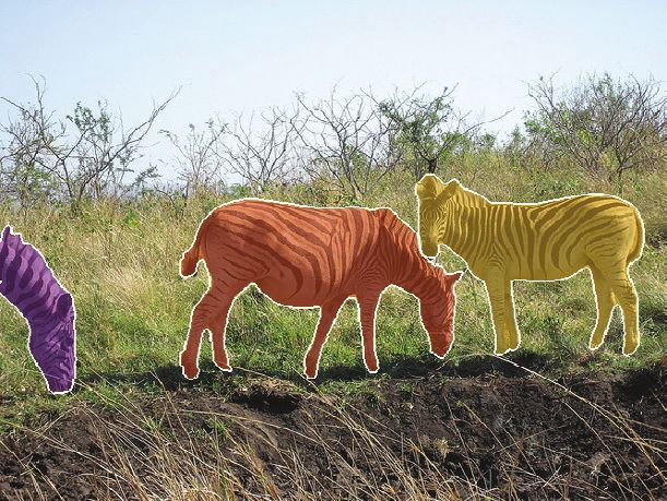
randomly sampling kN points (k>1) from a uniform distri-            are similar to the outputs made by the existing architectures,
bution. (ii) Importance sampling: we focus on points with           and are supervised during training in the same way as exist-
uncertain coarse predictions by interpolating the coarse            ing models. For instance segmentation, the coarse predic-
prediction values at all kN points and computing a task-            tion can be, for example, the output of a lightweight 7×7
specific uncertainty estimate (defined in §4 and §5). The           resolution mask head in Mask R-CNN. For semantic seg-
most uncertain βN points (β ∈ [0, 1]) are selected from             mentation, it can be, for example, predictions from a stride
the kN candidates. (iii) Coverage: the remaining (1 − β)N           16 feature map.
points are sampled from a uniform distribution. We illus-
                                                                    Point head. Given the point-wise feature representation
trate this procedure with different settings, and compare it
                                                                    at each selected point, PointRend makes point-wise seg-
to regular grid selection, in Fig. 5.
                                                                    mentation predictions using a simple multi-layer percep-
    At training time, predictions and loss functions are only
                                                                    tron (MLP). This MLP shares weights across all points (and
computed on the N sampled points (in addition to the coarse
                                                                    all regions), analogous to a graph convolution [23] or a
segmentation), which is simpler and more efficient than
                                                                    PointNet [43]. Since the MLP predicts a segmentation la-
backpropagation through subdivision steps. This design is
                                                                    bel for each point, it can be trained by standard task-specific
similar to the parallel training of RPN + Fast R-CNN in a
                                                                    segmentation losses (described in §4 and §5).
Faster R-CNN system [13], whose inference is sequential.

3.2. Point-wise Representation and Point Head                       4. Experiments: Instance Segmentation
   PointRend constructs point-wise features at selected             Datasets. We use two standard instance segmentation
points by combining (e.g., concatenating) two feature types,        datasets: COCO [29] and Cityscapes [9]. We report the
fine-grained and coarse prediction features, described next.        standard mask AP metric [29] using the median of 3 runs
                                                                    for COCO and 5 for Cityscapes (it has higher variance).
Fine-grained features. To allow PointRend to render fine               COCO has 80 categories with instance-level annotation.
segmentation details we extract a feature vector at each sam-       We train on train2017 (∼118k images) and report results
pled point from CNN feature maps. Because a point is a              on val2017 (5k images). As noted in [16], the COCO
real-value 2D coordinate, we perform bilinear interpolation         ground-truth is often coarse and AP for the dataset may not
on the feature maps to compute the feature vector, follow-          fully reflect improvements in mask quality. Therefore we
ing standard practice [22, 19, 10]. Features can be extracted       supplement COCO results with AP measured using the 80
from a single feature map (e.g., res2 in a ResNet); they can        COCO category subset of LVIS [16], denoted by AP? . The
also be extracted from multiple feature maps (e.g., res2 to         LVIS annotations have significantly higher quality. Note
res5 , or their feature pyramid [28] counterparts) and con-         that for AP? we use the same models trained on COCO
catenated, following the Hypercolumn method [17].                   and simply re-evaluate their predictions against the higher-
Coarse prediction features. The fine-grained features en-           quality LVIS annotations using the LVIS evaluation API.
able resolving detail, but are also deficient in two regards.          Cityscapes is an ego-centric street-scene dataset with
First, they do not contain region-specific information and          8 categories, 2975 train images, and 500 validation im-
thus the same point overlapped by two instances’ bound-             ages. The images are higher resolution compared to COCO
ing boxes will have the same fine-grained features. Yet, the        (1024×2048 pixels) and have finer, more pixel-accurate
point can only be in the foreground of one instance. There-         ground-truth instance segmentations.
fore, for the task of instance segmentation, where different        Architecture. Our experiments use Mask R-CNN with a
regions may predict different labels for the same point, ad-        ResNet-50 [20] + FPN [28] backbone. The default mask
ditional region-specific information is needed.                     head in Mask R-CNN is a region-wise FCN, which we de-
    Second, depending on which feature maps are used for            note by “4× conv”.2 We use this as our baseline for com-
the fine-grained features, the features may contain only rel-       parison. For PointRend, we make appropriate modifications
atively low-level information (e.g., we will use res2 with          to this baseline, as described next.
DeepLabV3). In this case, a feature source with more con-
textual and semantic information can be helpful. This issue         Lightweight, coarse mask prediction head. To compute
affects both instance and semantic segmentation.                    the coarse prediction, we replace the 4× conv mask head
    Based on these considerations, the second feature type is       with a lighter weight design that resembles Mask R-CNN’s
a coarse segmentation prediction from the network, i.e., a          box head and produces a 7×7 mask prediction. Specifi-
K-dimensional vector at each point in the region (box) rep-         cally, for each bounding box, we extract a 14×14 feature
resenting a K-class prediction. The coarse resolution, by               2 Four layers of 3×3 convolutions with 256 output channels are applied
design, provides more globalized context, while the chan-           to a 14×14 input feature map. Deconvolution with a 2×2 kernel trans-
nels convey the semantic classes. These coarse predictions          forms this to 28×28. Finally, a 1×1 convolution predicts mask logits.

                                                                5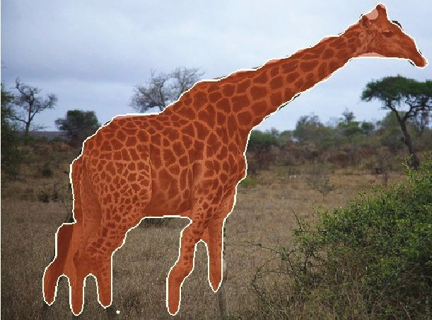
map from the P2 level of the FPN using bilinear interpola-                               output             COCO              Cityscapes
tion. The features are computed on a regular grid inside the            mask head      resolution      AP         AP?             AP
bounding box (this operation can seen as a simple version of            4× conv          28×28      35.2        37.6          33.0
RoIAlign). Next, we use a stride-two 2×2 convolution layer              PointRend        28×28      36.1 (+0.9) 39.2 (+1.6)   35.5 (+2.5)
                                                                        PointRend      224×224      36.3 (+1.1) 39.7 (+2.1)   35.8 (+2.8)
with 256 output channels followed by ReLU [39], which
reduces the spatial size to 7×7. Finally, similar to Mask            Table 1: PointRend vs. the default 4× conv mask head for Mask
R-CNN’s box head, an MLP with two 1024-wide hidden                   R-CNN [19]. Mask AP is reported. AP? is COCO mask AP eval-
layers is applied to yield a 7×7 mask prediction for each of         uated against the higher-quality LVIS annotations [16] (see text
the K classes. ReLU is used on the MLP’s hidden layers               for details). A ResNet-50-FPN backbone is used for both COCO
and the sigmoid activation function is applied to its outputs.       and Cityscapes models. PointRend outperforms the standard 4×
                                                                     conv mask head both quantitively and qualitatively. Higher output
PointRend. At each selected point, a K-dimensional fea-              resolution leads to more detailed predictions, see Fig. 2 and Fig. 6.
ture vector is extracted from the coarse prediction head’s
output using bilinear interpolation. PointRend also interpo-
lates a 256-dimensional feature vector from the P2 level of
the FPN. This level has a stride of 4 w.r.t. the input image.

                                                                     28×28
These coarse prediction and fine-grained feature vectors are
concatenated. We make a K-class prediction at selected
points using an MLP with 3 hidden layers with 256 chan-
nels. In each layer of the MLP, we supplement the 256 out-
put channels with the K coarse prediction features to make           224×224
the input vector for the next layer. We use ReLU inside the
MLP and apply sigmoid to its output.
Training. We use the standard 1× training schedule and
data augmentation from Detectron2 [49] by default (full de-          Figure 6: PointRend inference with different output resolu-
tails are in the appendix). For PointRend, we sample 142             tions. High resolution masks align better with object boundaries.
points using the biased sampling strategy described in the
§3.1 with k=3 and β=0.75. We use the distance between                          mask head   output resolution   FLOPs    # activations
0.5 and the probability of the ground truth class interpo-                     4× conv         28×28            0.5B        0.5M
lated from the coarse prediction as the point-wise uncer-                      4× conv        224×224           34B         33M
tainty measure. For a predicted box with ground-truth class                    PointRend      224×224           0.9B        0.7M
c, we sum the binary cross-entropy loss for the c-th MLP
output over the 142 points. The lightweight coarse predic-           Table 2: FLOPs (multiply-adds) and activation counts for a
tion head uses the average cross-entropy loss for the mask           224×224 output resolution mask. PointRend’s efficient subdi-
                                                                     vision makes 224×224 output feasible in contrast to the standard
predicted for class c, i.e., the same loss as the baseline 4×
                                                                     4× conv mask head modified to use an RoIAlign size of 112×112.
conv head. We sum all losses without any re-weighting.
    During training, Mask R-CNN applies the box and mask
heads in parallel, while during inference they run as a cas-         ing the COCO categories using the LVIS annotations (AP? )
cade. We found that training as a cascade does not improve           and for Cityscapes, which we attribute to the superior anno-
the baseline Mask R-CNN, but PointRend can benefit from              tation quality in these datasets. Even with the same output
it by sampling points inside more accurate boxes, slightly           resolution PointRend outperforms the baseline. The differ-
improving overall performance (∼0.2% AP, absolute).                  ence between 28×28 and 224×224 is relatively small be-
                                                                     cause AP uses intersection-over-union [11] and, therefore,
Inference. For inference on a box with predicted class c,            is heavily biased towards object-interior pixels and less sen-
unless otherwise specified, we use the adaptive subdivision          sitive to the boundary quality. Visually, however, the differ-
technique to refine the coarse 7×7 prediction for class c to         ence in boundary quality is obvious, see Fig. 6.
the 224×224 in 5 steps. At each step, we select and update
(at most) the N =282 most uncertain points based on the              Subdivision inference allows PointRend to yield a high
absolute difference between the predictions and 0.5.                 resolution 224×224 prediction using more than 30 times
                                                                     less compute (FLOPs) and memory than the default 4×
4.1. Main Results
                                                                     conv head needs to output the same resolution (based on
   We compare PointRend to the default 4× conv head in               taking a 112×112 RoIAlign input), see Table 2. PointRend
Mask R-CNN in Table 1. PointRend outperforms the de-                 makes high resolution output feasible in the Mask R-CNN
fault head on both datasets. The gap is larger when evaluat-         framework by ignoring areas of an object where a coarse

                                                                 6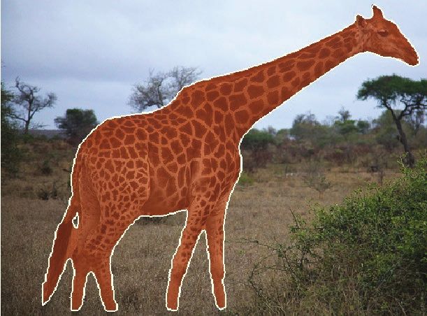
# points per        COCO        Cityscapes                                                COCO         Cityscapes
output resolution   subdivision step    AP AP?            AP                 selection strategy               AP AP?             AP
    28×28                 282           36.1 39.2        35.4                regular grid                     35.7 39.1         34.4
    56×56                 282           36.2 39.6        35.8                uniform (k=1, β=0.0)             35.9 39.0         34.5
   112×112                282           36.3 39.7        35.8                mildly biased (k=3, β=0.75)      36.3 39.7         35.8
   224×224                282           36.3 39.7        35.8                heavily biased (k=10, β=1.0)     34.4 37.5         34.1
   224×224                142           36.1 39.4        35.5
                                                                          Table 4: Training-time point selection strategies with 142 points
   224×224                282           36.3 39.7        35.8
                                                                          per box. Mildly biasing sampling towards uncertain regions per-
   224×224                562           36.3 39.7        35.8
                                                                          forms the best. Heavily biased sampling performs even worse than
   224×224               1122           36.3 39.7        35.8
                                                                          uniform or regular grid sampling indicating the importance of cov-
Table 3: Subdivision inference parameters. Higher output res-             erage. AP? is COCO mask AP evaluated against the higher-quality
olution improves AP. Although improvements saturate quickly (at           LVIS annotations [16] (see text for details).
underlined values) with the number of points sampled at each sub-
division step, qualitative results may continue to improve for com-                                                 COCO
plex objects. AP? is COCO mask AP evaluated against the higher-                   mask head    backbone         AP         AP?
quality LVIS annotations [16] (see text for details).                             4× conv      R50-FPN       37.2        39.5
                                                                                  PointRend    R50-FPN       38.2 (+1.0) 41.5 (+2.0)
    28×28            56×56          112×112           224×224                     4× conv      R101-FPN      38.6        41.4
                                                                                  PointRend    R101-FPN      39.8 (+1.2) 43.5 (+2.1)
                                                                                  4× conv      X101-FPN      39.5        42.1
                                                                                  PointRend    X101-FPN      40.9 (+1.4) 44.9 (+2.8)

                                                                          Table 5: Larger models and a longer 3× schedule [18].
                                                                          PointRend benefits from more advanced models and the longer
                                                                          training. The gap between PointRend and the default mask head
                                                                          in Mask R-CNN holds. AP? is COCO mask AP evaluated against
                                                                          the higher-quality LVIS annotations [16] (see text for details).

                                                                          4.2. Ablation Experiments
                                                                             We conduct a number of ablations to analyze PointRend.
Figure 7: Anti-aliasing with PointRend. Precise object delin-             In general we note that it is robust to the exact design of the
eation requires output mask resolution to match or exceed the res-        point head MLP. Changes of its depth or width do not show
olution of the input image region that the object occupies.               any significant difference in our experiments.
                                                                          Point selection during training. During training we select
prediction is sufficient (e.g., in the areas far away from ob-            142 points per object following the biased sampling strat-
ject boundaries). In terms of wall-clock runtime, our unop-               egy (§3.1). Sampling only 142 points makes training com-
timized implementation outputs 224×224 masks at ∼13 fps,                  putationally and memory efficient and we found that using
which is roughly the same frame-rate as a 4× conv head                    more points does not improve results. Surprisingly, sam-
modified to output 56×56 masks (by doubling the default                   pling only 49 points per box still maintains AP, though we
RoIAlign size), a design that actually has lower COCO AP                  observe an increased variance in AP.
compared to the 28×28 4× conv head (34.5% vs. 35.2%).                        Table 4 shows PointRend performance with different se-
                                                                          lection strategies during training. Regular grid selection
   Table 3 shows PointRend subdivision inference with dif-
                                                                          achieves similar results to uniform sampling. Whereas bias-
ferent output resolutions and number of points selected at
                                                                          ing sampling toward ambiguous areas improves AP. How-
each subdivision step. Predicting masks at a higher res-
                                                                          ever, a sampling strategy that is biased too heavily towards
olution can improve results. Though AP saturates, visual
                                                                          boundaries of the coarse prediction (k>10 and β close to
improvements are still apparent when moving from lower
                                                                          1.0) decreases AP. Overall, we find a wide range of param-
(e.g., 56×56) to higher (e.g., 224×224) resolution outputs,
                                                                          eters 2
Mask R-CNN + 4×conv                Mask R-CNN + PointRend                        DeeplabV3                   DeeplabV3 + PointRend

Figure 8: Cityscapes example results for instance and semantic segmentation. In instance segmentation larger objects benefit more
from PointRend ability to yield high resolution output. Whereas for semantic segmentation PointRend recovers small objects and details.

5. Experiments: Semantic Segmentation                                         method                             output resolution   mIoU
                                                                              DeeplabV3-OS-16                        64×128          77.2
   PointRend is not limited to instance segmentation and                      DeeplabV3-OS-8                        128×256          77.8 (+0.6)
can be extended to other pixel-level recognition tasks. Here,                 DeeplabV3-OS-16 + PointRend          1024×2048         78.4 (+1.2)
we demonstrate that PointRend can benefit two semantic
                                                                              Table 6: DeeplabV3 with PointRend for Cityscapes semantic
segmentation models: DeeplabV3 [5], which uses dilated
                                                                              segmentation outperforms baseline DeepLabV3. Dilating the res4
convolutions to make prediction on a denser grid, and Se-                     stage during inference yields a larger, more accurate prediction,
manticFPN [24], a simple encoder-decoder architecture.                        but at much higher computational and memory costs; it is still in-
Dataset. We use the Cityscapes [9] semantic segmentation                      ferior to using PointRend.
set with 19 categories, 2975 training images, and 500 vali-
dation images. We report the median mIoU of 5 trials.
Implementation details. We reimplemented DeeplabV3
and SemanticFPN following their respective papers. Se-
manticFPN uses a standard ResNet-101 [20], whereas
DeeplabV3 uses the ResNet-103 proposed in [5].3 We fol-
low the original papers’ training schedules and data aug-
mentation (details are in the appendix).
   We use the same PointRend architecture as for in-                          Figure 9: PointRend inference for semantic segmentation.
stance segmentation. Coarse prediction features come from                     PointRend refines prediction scores for areas where a coarser pre-
the (already coarse) output of the semantic segmentation                      diction is not sufficient. To visualize the scores at each step we
model. Fine-grained features are interpolated from res2 for                   take arg max at given resolution without bilinear interpolation.
DeeplabV3 and from P2 for SemanticFPN. During training
                                                                              method                         output resolution       mIoU
we sample as many points as there are on a stride 16 fea-
                                                                              SemanticFPN P2 -P5                256×512              77.7
ture map of the input (2304 for deeplabV3 and 2048 for Se-                    SemanticFPN P2 -P5 + PointRend   1024×2048             78.6 (+0.9)
manticFPN). We use the same k=3, β=0.75 point selection                       SemanticFPN P3 -P5                128×256              77.4
strategy. During inference, subdivision uses N =8096 (i.e.,                   SemanticFPN P3 -P5 + PointRend   1024×2048             78.5 (+1.1)
the number of points in the stride 16 map of a 1024×2048
image) until reaching the input image resolution. To mea-                     Table 7: SemanticFPN with PointRend for Cityscapes semantic
sure prediction uncertainty we use the same strategy dur-                     segmentation outperform the baseline SemanticFPN.
ing training and inference: the difference between the most
confident and second most confident class probabilities.
                                                                              PointRend has higher mIoU. Qualitative improvements are
DeeplabV3. In Table 6 we compare DeepLabV3 to                                 also evident, see Fig. 8. By sampling points adaptively,
DeeplabV3 with PointRend. The output resolution can also                      PointRend reaches 1024×2048 resolution (i.e. 2M points)
be increased by 2× at inference by using dilated convolu-                     by making predictions for only 32k points, see Fig. 9.
tions in res4 stage, as described in [5]. Compared to both,                   SemanticFPN. Table 7 shows that SemanticFPN with
   3 Itreplaces the ResNet-101 res1 7×7 convolution with three 3×3 con-       PointRend improves over both 8× and 4× output stride
volutions (hence “ResNet-103”).                                               variants without PointRend.

                                                                          8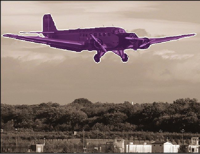
Appendix A. Instance Segmentation Details                              Appendix C. AP? Computation
   We use SGD with 0.9 momentum; a linear learning rate                   The first version (v1) of this paper on arXiv has an er-
warmup [15] over 1000 updates starting from a learning rate            ror in COCO mask AP evaluated against the LVIS annota-
of 0.001 is applied; weight decay 0.0001 is applied; hori-             tions [16] (AP? ). The old version used an incorrect list of
zontal flipping and scale train-time data augmentation; the            the categories not present in each evaluation image, which
batch normalization (BN) [21] layers from the ImageNet                 resulted in lower AP? values.
pre-trained models are frozen (i.e., BN is not used); no test-
time augmentation is used.                                             References
COCO [29]: 16 images per mini-batch; the training sched-                [1] Anurag Arnab and Philip HS Torr. Pixelwise instance
ule is 60k / 20k / 10k updates at learning rates of 0.02 / 0.002            segmentation with a dynamically instantiated network. In
                                                                            CVPR, 2017. 3
/ 0.0002 respectively; training images are resized randomly
to a shorter edge from 640 to 800 pixels with a step of 32              [2] Samuel Rota Bulò, Lorenzo Porzi, and Peter Kontschieder.
                                                                            In-place activated batchnorm for memory-optimized training
pixels and inference images are resized to a shorter edge
                                                                            of DNNs. In CVPR, 2018. 9
size of 800 pixels.
                                                                        [3] Kai Chen, Jiangmiao Pang, Jiaqi Wang, Yu Xiong, Xiaox-
                                                                            iao Li, Shuyang Sun, Wansen Feng, Ziwei Liu, Jianping Shi,
Cityscapes [9]: 8 images per mini-batch the training                        Wanli Ouyang, et al. Hybrid task cascade for instance seg-
schedule is 18k / 6k updates at learning rates of 0.01 /                    mentation. In CVPR, 2019. 3
0.001 respectively; training images are resized randomly to             [4] Liang-Chieh Chen, George Papandreou, Iasonas Kokkinos,
a shorter edge from 800 to 1024 pixels with a step of 32 pix-               Kevin Murphy, and Alan L Yuille. DeepLab: Semantic im-
els and inference images are resized to a shorter edge size                 age segmentation with deep convolutional nets, atrous con-
of 1024 pixels.                                                             volution, and fully connected CRFs. PAMI, 2018. 3
                                                                        [5] Liang-Chieh Chen, George Papandreou, Florian Schroff, and
Longer schedule: The 3× schedule for COCO is 210k /                         Hartwig Adam. Rethinking atrous convolution for semantic
40k / 20k updates at learning rates of 0.02 / 0.002 / 0.0002,               image segmentation. arXiv:1706.05587, 2017. 2, 3, 8, 9
respectively; all other details are the same as the setting de-         [6] Liang-Chieh Chen, Yukun Zhu, George Papandreou, Florian
scribed above.                                                              Schroff, and Hartwig Adam. Encoder-decoder with atrous
                                                                            separable convolution for semantic image segmentation. In
                                                                            ECCV, 2018. 3
Appendix B. Semantic Segmentation Details
                                                                        [7] Xinlei Chen, Ross Girshick, Kaiming He, and Piotr Dollár.
DeeplabV3 [5]: We use SGD with 0.9 momentum with 16                         TensorMask: A foundation for dense object segmentation. In
images per mini-batch cropped to a fixed 768×768 size;                      ICCV, 2019. 3
the training schedule is 90k updates with a poly learning               [8] Christopher B Choy, Danfei Xu, JunYoung Gwak, Kevin
rate [34] update strategy, starting from 0.01; a linear learn-              Chen, and Silvio Savarese. 3D-R2N2: A unified approach
ing rate warmup [15] over 1000 updates starting from a                      for single and multi-view 3D object reconstruction. In
                                                                            ECCV, 2016. 3
learning rate of 0.001 is applied; the learning rate for ASPP
and the prediction convolution are multiplied by 10; weight             [9] Marius Cordts, Mohamed Omran, Sebastian Ramos, Timo
                                                                            Rehfeld, Markus Enzweiler, Rodrigo Benenson, Uwe
decay of 0.0001 is applied; random horizontal flipping and
                                                                            Franke, Stefan Roth, and Bernt Schiele. The Cityscapes
scaling of 0.5× to 2.0× with a 32 pixel step is used as train-              dataset for semantic urban scene understanding. In CVPR,
ing data augmentation; BN is applied to 16 images mini-                     2016. 2, 3, 5, 8, 9
batches; no test-time augmentation is used;                            [10] Jifeng Dai, Haozhi Qi, Yuwen Xiong, Yi Li, Guodong
                                                                            Zhang, Han Hu, and Yichen Wei. Deformable convolutional
SemanticFPN [24]: We use SGD with 0.9 momentum                              networks. In ICCV, 2017. 5
with 32 images per mini-batch cropped to a fixed 512×1024              [11] Mark Everingham, SM Ali Eslami, Luc Van Gool, Christo-
size; the training schedule is 40k / 15k / 10k updates at                   pher KI Williams, John Winn, and Andrew Zisserman. The
learning rates of 0.01 / 0.001 / 0.0001 respectively; a linear              PASCAL visual object classes challenge: A retrospective.
learning rate warmup [15] over 1000 updates starting from                   IJCV, 2015. 6
a learning rate of 0.001 is applied; weight decay 0.0001 is            [12] Rohit Girdhar, David F Fouhey, Mikel Rodriguez, and Ab-
applied; horizontal flipping, color augmentation [33], and                  hinav Gupta. Learning a predictable and generative vector
crop bootstrapping [2] are used during training; scale train-               representation for objects. In ECCV, 2016. 3
time data augmentation resizes an input image from 0.5×                [13] Ross Girshick. Fast R-CNN. In ICCV, 2015. 5
to 2.0× with a 32 pixel step; BN layers are frozen (i.e., BN           [14] Georgia Gkioxari, Jitendra Malik, and Justin Johnson. Mesh
is not used); no test-time augmentation is used.                            R-CNN. In ICCV, 2019. 3

                                                                   9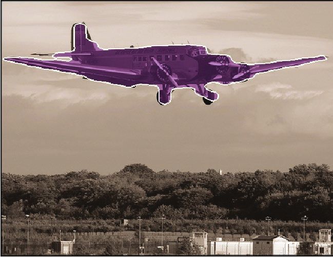
[15] Priya Goyal, Piotr Dollár, Ross Girshick, Pieter Noord-             [33] Wei Liu, Dragomir Anguelov, Dumitru Erhan, Christian
     huis, Lukasz Wesolowski, Aapo Kyrola, Andrew Tulloch,                     Szegedy, Scott Reed, Cheng-Yang Fu, and Alexander C
     Yangqing Jia, and Kaiming He. Accurate, large minibatch                   Berg. SSD: Single shot multibox detector. In ECCV, 2016.
     sgd: Training imagenet in 1 hour. arXiv:1706.02677, 2017.                 9
     9                                                                    [34] Wei Liu, Andrew Rabinovich, and Alexander C Berg.
[16] Agrim Gupta, Piotr Dollar, and Ross Girshick. LVIS: A                     Parsenet: Looking wider to see better. arXiv:1506.04579,
     dataset for large vocabulary instance segmentation. In ICCV,              2015. 9
     2019. 5, 6, 7, 9                                                     [35] Jonathan Long, Evan Shelhamer, and Trevor Darrell. Fully
[17] Bharath Hariharan, Pablo Arbeláez, Ross Girshick, and Ji-                convolutional networks for semantic segmentation. In
     tendra Malik. Hypercolumns for object segmentation and                    CVPR, 2015. 1, 2, 3, 4
     fine-grained localization. In CVPR, 2015. 5                          [36] Dmitrii Marin, Zijian He, Peter Vajda, Priyam Chatterjee,
[18] Kaiming He, Ross Girshick, and Piotr Dollár. Rethinking                  Sam Tsai, Fei Yang, and Yuri Boykov. Efficient segmenta-
     imagenet pre-training. In ICCV, 2019. 7                                   tion: Learning downsampling near semantic boundaries. In
                                                                               ICCV, 2019. 3
[19] Kaiming He, Georgia Gkioxari, Piotr Dollár, and Ross Gir-
     shick. Mask R-CNN. In ICCV, 2017. 1, 2, 3, 4, 5, 6                   [37] Lars Mescheder, Michael Oechsle, Michael Niemeyer, Se-
                                                                               bastian Nowozin, and Andreas Geiger. Occupancy networks:
[20] Kaiming He, Xiangyu Zhang, Shaoqing Ren, and Jian Sun.
                                                                               Learning 3d reconstruction in function space. In CVPR,
     Deep residual learning for image recognition. In CVPR,
                                                                               2019. 3
     2016. 2, 5, 8
                                                                          [38] Don P Mitchell. Generating antialiased images at low sam-
[21] Sergey Ioffe and Christian Szegedy. Batch normalization:                  pling densities. ACM SIGGRAPH Computer Graphics, 1987.
     Accelerating deep network training by reducing internal co-               2
     variate shift. In ICML, 2015. 9
                                                                          [39] Vinod Nair and Geoffrey E Hinton. Rectified linear units
[22] Max Jaderberg, Karen Simonyan, Andrew Zisserman, and                      improve restricted boltzmann machines. In ICML, 2010. 6
     Koray Kavukcuoglu. Spatial transformer networks. In NIPS,            [40] Gerhard Neuhold, Tobias Ollmann, Samuel Rota Bulò, and
     2015. 5                                                                   Peter Kontschieder. The mapillary vistas dataset for semantic
[23] Thomas N Kipf and Max Welling. Semi-supervised classifi-                  understanding of street scenes. In CVPR, 2017. 3
     cation with graph convolutional networks. ICLR, 2017. 5              [41] Paphio.       Jo-Wilfried Tsonga [19]. CC BY-NC-SA
[24] Alexander Kirillov, Ross Girshick, Kaiming He, and Piotr                  2.0. https://www.flickr.com/photos/paphio/
     Dollár. Panoptic feature pyramid networks. In CVPR, 2019.                2855627782/, 2008. 1
     3, 8, 9                                                              [42] Matt Pharr, Wenzel Jakob, and Greg Humphreys. Physically
[25] Alexander Kirillov, Evgeny Levinkov, Bjoern Andres, Bog-                  based rendering: From theory to implementation, chapter 7.
     dan Savchynskyy, and Carsten Rother. InstanceCut: from                    Morgan Kaufmann, 2016. 2
     edges to instances with multicut. In CVPR, 2017. 3                   [43] Charles R Qi, Hao Su, Kaichun Mo, and Leonidas J Guibas.
[26] Alex Krizhevsky, Ilya Sutskever, and Geoff Hinton. Im-                    PointNet: Deep learning on point sets for 3D classification
     ageNet classification with deep convolutional neural net-                 and segmentation. In CVPR, 2017. 5
     works. In NIPS, 2012. 1                                              [44] Olaf Ronneberger, Philipp Fischer, and Thomas Brox. U-
[27] Yann LeCun, Bernhard Boser, John S Denker, Donnie                         Net: Convolutional networks for biomedical image segmen-
     Henderson, Richard E Howard, Wayne Hubbard, and                           tation. In MICCAI, 2015. 3
     Lawrence D Jackel. Backpropagation applied to handwrit-              [45] Ke Sun, Yang Zhao, Borui Jiang, Tianheng Cheng, Bin Xiao,
     ten zip code recognition. Neural computation, 1989. 1                     Dong Liu, Yadong Mu, Xinggang Wang, Wenyu Liu, and
[28] Tsung-Yi Lin, Piotr Dollár, Ross Girshick, Kaiming He,                   Jingdong Wang. High-resolution representations for labeling
     Bharath Hariharan, and Serge Belongie. Feature pyramid                    pixels and regions. arXiv:1904.04514, 2019. 3
     networks for object detection. In CVPR, 2017. 2, 5                   [46] Maxim Tatarchenko, Alexey Dosovitskiy, and Thomas Brox.
[29] Tsung-Yi Lin, Michael Maire, Serge Belongie, James Hays,                  Octree generating networks: Efficient convolutional archi-
     Pietro Perona, Deva Ramanan, Piotr Dollár, and C Lawrence                tectures for high-resolution 3D outputs. In ICCV, 2017. 3
     Zitnick. Microsoft COCO: Common objects in context. In               [47] Nanyang Wang, Yinda Zhang, Zhuwen Li, Yanwei Fu, Wei
     ECCV, 2014. 2, 3, 5, 9                                                    Liu, and Yu-Gang Jiang. Pixel2Mesh: Generating 3D mesh
                                                                               models from single RGB images. In ECCV, 2018. 3
[30] Chenxi Liu, Liang-Chieh Chen, Florian Schroff, Hartwig
     Adam, Wei Hua, Alan L Yuille, and Li Fei-Fei. Auto-                  [48] Turner Whitted. An improved illumination model for shaded
     deeplab: Hierarchical neural architecture search for semantic             display. In ACM SIGGRAPH Computer Graphics, 1979. 2,
     image segmentation. In CVPR, 2019. 3                                      4
                                                                          [49] Yuxin Wu, Alexander Kirillov, Francisco Massa, Wan-Yen
[31] Shu Liu, Jiaya Jia, Sanja Fidler, and Raquel Urtasun. SGN:
                                                                               Lo, and Ross Girshick. Detectron2. https://github.
     Sequential grouping networks for instance segmentation. In
                                                                               com/facebookresearch/detectron2, 2019. 6
     CVPR, 2017. 3
                                                                          [50] Kun Zhou, Qiming Hou, Rui Wang, and Baining Guo. Real-
[32] Shu Liu, Lu Qi, Haifang Qin, Jianping Shi, and Jiaya Jia.
                                                                               time kd-tree construction on graphics hardware. In ACM
     Path aggregation network for instance segmentation. In
                                                                               Transactions on Graphics (TOG), 2008. 2
     CVPR, 2018. 3

                                                                     10
You can also read