The Horus WLAN Location Determination System
←
→
Page content transcription
If your browser does not render page correctly, please read the page content below
The Horus WLAN Location Determination System

                                              Moustafa Youssef∗ and Ashok Agrawala
                                                Department of Computer Science
                                                     University of Maryland
                                                 College Park, Maryland 20742
                                               {moustafa, agrawala}@cs.umd.edu

Abstract                                                         currently implemented as a client-based system. A large
We present the design and implementation of the Horus            class of applications [10], including location-sensitive
WLAN location determination system. The design of the            content delivery, direction finding, asset tracking, and
Horus system aims at satisfying two goals: high accuracy         emergency notification, can be built on top of the Horus
and low computational requirements. The Horus system             system.
identifies different causes for the wireless channel varia-         WLAN location determination is an active research
tions and addresses them to achieve its high accuracy. It        area [5, 6, 8, 9, 12, 13, 15, 17, 20–22, 29–31, 33, 34].
uses location-clustering techniques to reduce the compu-         WLAN location determination systems usually work in
tational requirements of the algorithm. The lightweight          two phases: an offline training phase and an online lo-
Horus algorithm helps in supporting a larger number of           cation determination phase. During the offline phase, the
users by running the algorithm at the clients.                   system tabulates the signal strength received from the ac-
   We discuss the different components of the Horus sys-         cess points at selected locations in the area of interest,
tem and its implementation under two different operating         resulting in a so-called radio map. During the location
systems and evaluate the performance of the Horus sys-           determination phase, the system use the signal strength
tem on two testbeds. Our results show that the Horus             samples received from the access points to “search” the
system achieves its goal. It has an error of less than 0.6       radio map to estimate the user location.
meter on the average and its computational requirements             Radio-map based techniques can be categorized into
are more than an order of magnitude better than other            two broad categories: deterministic techniques and prob-
WLAN location determination systems. Moreover, the               abilistic techniques. Deterministic techniques [5, 6, 22]
techniques developed in the context of the Horus sys-            represent the signal strength of an access point at a loca-
tem are general and can be applied to other WLAN lo-             tion by a scalar value, for example, the mean value, and
cation determination systems to enhance their accuracy.          use non-probabilistic approaches to estimate the user lo-
We also report lessons learned from experimenting with           cation. For example, in the Radar system [5, 6] the au-
the Horus system and provide directions for future work.         thors use nearest neighborhood techniques to infer the
                                                                 user location. On the other hand, probabilistic tech-
1      Introduction                                              niques [8, 9, 13, 17, 20, 21, 29–31, 33, 34] store informa-
                                                                 tion about the signal strength distributions from the ac-
Horus is an RF-based location determination system. It
                                                                 cess points in the radio map and use probabilistic tech-
is currently implemented in the context of 802.11 wire-
                                                                 niques to estimate the user location. For example, the
less LANs [25]. The system uses the signal strength ob-
                                                                 Nibble system [8, 9] uses a Bayesian Network approach
served for frames transmitted by the access points to in-
                                                                 to estimate the user location.
fer the user location. Since the wireless cards measure
                                                                    The Horus system lies in the probabilistic techniques
the signal strength information of the received frames as
                                                                 category. The design of the Horus system aims at satisfy-
part of their normal operation, this makes the Horus sys-
                                                                 ing two goals: high accuracy and low computational re-
tem a software solution on top of the wireless network
                                                                 quirements. The Horus system identifies different causes
infrastructure. There are two classes of WLAN location
                                                                 for the wireless channel variations and addresses them
determination systems: client-based and infrastructure-
                                                                 to achieve its high accuracy. It uses location-clustering
based. Both have their own set of applications. Horus is
                                                                 techniques to reduce the computational requirements of
    ∗ Also   affiliated with Alexandria University, Egypt.       the algorithm. The lightweight Horus algorithm allows
0.5 Lucent Orinoco silver network interface card (NIC) sup-
0.45
porting up to 11 Mbit/s data rate [3]. The Horus system
is implemented under both the Linux and Windows op-
0.4
erating systems.
0.35
For the Linux OS, we modified [1] the Lucent Wave-
Probability
0.3
lan driver so that it returns the signal strength of probe
0.25 response frames received from all access points in the
0.2 NIC range using active scanning [25]; our driver was the
0.15 first to support this feature.
0.1 The scanning process output is a list of the MAC ad-
0.05 dresses of the access points associated with the signal
0 strength observed in this scan (through probe response
-52 -50 -48 -46 -44 -42 -40 -38 -36 frames). Each scan’s result set represents a sample.
Signal Strength (dBm) We also developed a wireless API [1] that interfaces
with any device driver that supports the wireless exten-
Figure 1: An example of the normalized signal strength sions [2]. The device driver and the wireless API have
histogram from an access point. been available for public download and have been used
by others in wireless research.
For the Microsoft Windows operating system, we used
it to be implemented in energy-constrained devices. This a custom-built NDIS driver to obtain the signal strength
non-centralized implementation helps in supporting a from the wireless card (using active scanning). This
larger number of users. In this paper, we present the dif- gives us more control over the scanning process as de-
ferent components of the Horus system and show how scribed in Section 5.
they work together to achieve its goals. We discuss our We now describe the different causes of variations in
Horus implementation under two different operating sys- a wireless channel. We divide these causes into two cat-
tems and evaluate its performance on two different in- egories: temporal variations and spatial variations.
door testbeds. 2.2 Temporal variations
The rest of the paper is structured as follows: in the
next section, we describe the different causes of varia- This section describes how the wireless channel changes
tions in the wireless channel. In Section 3 we present over time when the user is standing at a fixed position.
the different components of the Horus system that deal 2.2.1 Samples from one access point
with the noisy characteristics of the wireless channel. We
present the results of testing the Horus system on two We measured the signal strength from a single access
different testbeds in Section 4. Section 5 presents our point over a five minute period. We took the samples one
experience while building the Horus system. In Section second apart for a total of 300 samples. Figure 1 shows
6 we discuss related work. Finally, Section 7 concludes the normalized histogram of the received signal strength.
the paper and provides directions for future work. In our experience, the histogram range can be as large as
10 dBm or more. This time variation of the channel can
2 Wireless Channel Characteristics be due to changes in the physical environment such as
people moving about [23].
In this section, we identify the different causes of vari- These variations suggest that the radio map should re-
ations in the wireless channel quality and how they af- flect this range of values to increase the accuracy. More-
fect the WLAN location determination systems. We are over, during the online phase, the system should use
mainly concerned with the variations that affect the re- more than one sample in the estimation process to have a
ceived signal strength. We start by describing our sam- better estimate of the signal strength at a location.
pling process. Then, we categorize the variations in the
wireless channel as temporal variations and spatial varia- 2.2.2 Samples Correlation
tions. We performed all the experiments in this section in Figure 2 shows the autocorrelation function of the sam-
a typical office building, measured during the day when ples collected from one access point (one sample per
people are around. second) at a fixed position. The figure shows that the
autocorrelation of consecutive samples (lag = 1) is as
2.1 Sampling Process high as 0.9. This high autocorrelation is expected as over
A key function required by all WLAN location determi- a short period of time the signal strength received from
nation systems is signal-strength sampling. We used a an access point at a particular location is relatively stable1 300
0.92
Receiver sensitivity
Number of Samples Collected
0.8 0.9
Autocorr. coeff.
0.88 250
Autocorrelation coefficient
0.86
0.6
0.84 200
0.82
0.4
0.8
0.78
150
0.2 0 1 2 3 4 5 6 7 8 9 10
Time (Seconds) 100
0
50
-0.2
0
-0.4
0 1000 2000 3000 4000 5000 6000 7000 8000 -95 -90 -85 -80 -75 -70 -65 -60 -55
Time (Seconds) Average Signal Strength (dBm)
Figure 2: An example of the autocorrelation between Figure 3: Relation between the average signal strength of
samples from an access point (one sample per second). an access point and the percentage of samples received
The sub-figure shows the autocorrelation for the first 10 from it during a 5-minute interval.
seconds.
scale variations and small-scale variations.
(modulo the changes in the environment discussed in the
previous section). 2.3.1 Large-Scale Variations
This high autocorrelation value has to be considered Figure 4 shows the average signal strength received from
when using multiple samples from one access point to an access point as the distance from it increases. The sig-
enhance accuracy. Assuming independence of samples nal strength varies over a long distance due to attenuation
from the same access point leads to the undesirable re- of the RF signal.
sult of degraded system performance as the number of Large-scale variations are desirable in RF-based sys-
samples is increased (as explained in Section 4) as in a tems as they lead to changing the signature stored in the
typical WLAN environment samples from the same AP radio map for different locations and, hence, better dif-
are highly correlated. ferentiation between these locations.
2.2.3 Samples from different access points 2.3.2 Small-Scale Variations
We performed an experiment to test the behavior of ac- These variations happen when the user moves over a
cess points with different average signal strength at the small distance (order of wavelength). This leads to
same location. During this experiment, we sampled the changes in the average received signal strength. For the
signal strength from each access point at the rate of one 802.11b networks working at the 2.4 GHz range, the
sample per second. Figure 3 shows the relation between wavelength is 12.5 cm and we measure a variation in the
the average signal strength received from an access point average signal strength up to 10 dBm in a distance as
and the percentage of samples we receive from it during small as 7.6 cm (3 inches) (Figure 5).
a period of 5 minutes. The figure shows that the number Dealing with small-scale variations is challenging. To
of samples collected from an access point is a monoton- limit the radio map size and the time required to build
ically increasing function of the average signal strength the radio map, selected radio map locations are typically
of this access point. Assuming a constant noise level, the placed more than a meter apart. This means that the ra-
higher the signal strength, the higher the signal to noise dio map does not capture small-scale variations leading
ratio and the more probable it becomes that the 802.11b to decreased accuracy in the current WLAN location sys-
card will identify the existence of a frame. The sharp tems.
drop at about -81 dBm can be explained by noting that
In the next section, we indicate how the Horus system
the receiver sensitivity (minimum signal power required
handles these temporal and spacial variations.
to detect a frame) for the card we used was -82 dBm.
2.3 Spatial characteristics 3 The Horus System
These variations occur when the receiver position is In this section, we present the different components of
changed. We further divide these variations into large- the Horus system.30 −60
4
-42 −6 8
−7
−6
4 −6
−70
2
8
Average Signal Strength (dBm)
-44
−6
−66
6
25 −6
−72
-46 −6 −6
−6
4
−6
8 6
4
-48 −62 −6
8
Y (centimeters)
−65
-50 20
6 8
−6 −6
−74
−7
-52
−68
−6
−6
0
−70
6
4
-54
−6
15 −66 −6
−7
4
6
2
−62
-56
−66
−6
0
−70
−60
−6
-58
8
2
−664
10 −
−
66
-60 8
−6
−7
−64
0
-62
−66
5
−68
2 4 6 8 10 12 14 16
−66
62
−6
4 −
6
Distance (Meter) 2 −75
−6 −6
8
−6
−70
−6
0
0
0 10 20 30 40 50
Figure 4: Large-scale variations: Average signal strength X (centimeters)
over distance.
Figure 5: Small-scale variations: Signal strength con-
tours from an AP in a 30.4 cm (12 inches) by 53.3 cm
3.1 Overview (21 inches) area.
Figure 6 shows the overall system. The Horus system
works in two phases:
The Small-Scale Compensator module handles the
1. Offline phase: to build the radio map, cluster ra-
small-scale variation characteristics of the wireless chan-
dio map locations, and do other preprocessing of the
nel (Section 3.6).
signal strength models.
We start by laying out the mathematical framework
2. Online Phase: to estimate the user location based on for the approach then give details about different com-
the received signal strength from each access point ponents of the system.
and the radio map prepared in the offline phase.
3.2 Mathematical Model
The radio map stores the distribution of signal strength Without loss of generality, let X be a 2 dimensional phys-
received from each access point at each sampled loca- ical space. At each location x ∈ X, we can get the
tion. There are two modes for operation of the Horus signal strength from k access points. We denote the k-
system: one uses non-parametric distributions and the dimensional signal strength space as S. Each element in
other uses parametric distributions. this space is a k-dimensional vector whose entries rep-
The Clustering module is used to group radio map lo- resent the signal strength readings from different access
cations based on the access points covering them. Clus- points. We denote samples from the signal strength space
tering is used to reduce the computational requirements S as s. We also assume that the samples from different
of the system and, hence, conserve power (Section 3.7). access points are independent.
The Discrete Space Estimator module returns the ra-
The problem becomes, given a signal strength vector
dio map location that has the maximum probability given
s = (s1 , ..., sk ), we want to find the location x ∈ X that
the received signal strength vector from different access
maximizes the probability P (x/s).
points (Section 3.3).
The Correlation Modelling and Handling modules use In the next section, we assume a discrete X space. We
an autoregressive model to capture the correlation be- discuss the continuous space case in Section 3.5.
tween consecutive samples from the same access point.
3.3 Discrete Space Estimator
This model is used to obtain a better discrete location es-
timate using the average of n correlated samples (Section During the offline phase, the Horus system estimates the
3.4). signal strength histogram for each access point at each
The Continuous Space Estimator takes as an input the location. These histograms represent the Horus system’s
discrete estimated user location, one of the radio map lo- radio map. Now consider the online phase. Given a sig-
cations, and returns a more accurate estimate of the user nal strength vector s = (s1 , ..., sk ), we want to find the
location in the continuous space (Section 3.5). location x ∈ X that maximizes the probability P (x/s),Applications one access point is as high as 0.9. Assuming indepen-
Estimated Location
dence of samples from the same access point leads to the
Location API
undesirable result of degraded system performance as the
number of averaged samples is increased (as we demon-
Continuous-Space strate below, in Section 4).
Estimator
Horus System Components
3.4.1 Mathematical model
Radio
Map Small-Scale
We use an autoregressive model to capture the correla-
and
clusters
Compensator tion between different samples from the same AP.
Let st be the stationary time series representing the
Discrete-Space
samples from an access point, where t is the discrete time
Correlation
Modeler
Estimator index. st can be represented as a first order autoregres-
sive model [7] as:
Radio Map
Builder Clustering
Correlation
Handler st = αst−1 + (1 − α)vt ;0 ≤ α ≤ 1 (4)
where vt is a noise process, independent of st , and α
Signal Strength Acquisition API is a parameter that determines the degree of autocorre-
(MAC, Signal Strength)
lation of the original samples. Moreover, different sam-
Device Driver ples from vt are independent and identically distributed
(i.i.d.).
The model in Equation 4 states that the current sig-
nal strength value (st ) is a linear aggregate of the previ-
ous signal strength value (st−1 ) and an independent noise
value (vt ). The parameter α gives flexibility to the model
as it can be used to determine the degree of autocorrela-
Figure 6: Horus Components: the arrows show infor- tion of the original process. For example, if α is zero, the
mation flow in the system. Shadowed blocks represent samples of the process st are i.i.d.’s, whereas if α is 1 the
modules used during the offline phase. original samples are identical (autocorrelation=1).
Assuming that the signal strength distribution of sam-
ples from an access point is Gaussian with mean µ and
variance σ 2 , we have shown in [29, 31] that the distribu-
i.e., we want tion of the average of n correlated samples is a Gaussian
argmaxx [P (x/s)] (1) distribution with mean µ and variance given by:
Using Bayes’ theorem, this can be shown to be equiva- 1+α 2
lent to [33]: σ (5)
1−α
argmaxx [P (x/s)] = argmaxx [P (s/x)] (2) 3.4.2 Correlation modeler
The purpose of the correlation modeler component is to
P (s/x) can be calculated using the radio map as:
estimate the value of α in the autoregressive model and
k to pre-calculate the parameters of the distribution of the
Y
P (s/x) = P (si /x) (3) average of n correlated samples during the offline phase.
i=1 In a previous work [29,31], we have shown that α can be
approximated using the autocorrelation coefficient with
The signal-strength histogram can be approximated by lag 1. The variance of the distribution can be calculated
a parametric distribution such as the Gaussian distribu- using Equation 5. These distribution parameters (µ, σ,
tion. We compare the performance of the discrete-space and α) are then stored in the radio map.
estimator based on the parametric and non-parametric
3.4.3 Correlation handler
distributions in the Section 4.
During the online phase, the correlation handler mod-
3.4 Correlation Handling ule averages the value of n consecutive samples from an
To account for the temporal signal-strength variations, it access point and passes this information to the discrete-
is important to average multiple signal strength samples space estimator, which uses the distributions stored in the
from the same access point. As we showed in Figure 2, radio map (taking correlation into account using the in-
the autocorrelation of successive samples collected from formation in Section 3.4.1) to estimate the user location.3.5 Continuous Space Estimator uses the Perturbation technique to handle the small-scale
The discrete-space estimator returns a single location variations. The technique is based on two sub-functions:
from the set of locations in the radio map. To increase the detecting small-scale variations and compensating for
system accuracy, the Horus system uses two techniques small-scale variations.
to obtain a location estimate in the continuous space. 3.6.1 Detecting small-scale variations
3.5.1 Technique 1: Center of Mass of the Top Can- In order to detect small-scale variations, the Horus sys-
didate Locations tem uses the heuristic that users’ location cannot change
This technique is based on treating each location in the faster than their movement rate. The system calculates
radio map as an object in the physical space whose the estimated location using the standard radio map and
weight is equal to the normalized probability1 assigned the inference algorithm, then calculates the distance be-
by the discrete-space estimator. We then obtain the cen- tween the estimated location and the previous user loca-
ter of mass of the N objects with the largest mass, where tion. If this distance is above a threshold, based on the
N is a parameter to the system, 1 ≤ N ≤ ||X||. user movement rate and estimation frequency, the system
More formally, let p(x) be the probability of a location decides that there are small-scale variations affecting the
x ∈ X, i.e., the radio map, and let X̄ be the list of loca- signal strength.
tions in the radio map ordered in a descending order ac- 3.6.2 Compensating for small-scale variations
cording to the normalized probability (the location with To compensate for these small-scale variations, the sys-
lower ID comes first for locations with equal probabil- tem perturbs the received vector entries, re-estimates the
ity). The center of mass technique estimates the current location, and chooses the nearest location to the previous
location x as: user location as the final location estimate. For exam-
P
N ple, if one sample includes a signal-strength observation
p(i)X̄(i) from each of k access points (s1 , s2 , . . . , sk ), the system
i=1
x= tries all 3k combinations in which each of the k observa-
PN
(6)
p(i) tions i is replaced by one of three values, si , si (1 + d), or
i=1
si (1 − d); we explore the parameter d in Section 4.2.4.
where X̄(i) is the ith element of X̄ An enhancement of this approach is to perturb a subset
of the access points. The effect of the number of access
Note that the estimated location x need not be one of the
points to perturb and the value of d on accuracy is de-
radio map locations.
scribed in Section 4.
3.5.2 Technique 2: Time-Averaging in the Physical
Space 3.7 Clustering Module
The second technique uses a time-average window to This section describes the Incremental Triangulation
smooth the resulting location estimate. The technique (IT) clustering technique used by the Horus system to re-
obtains the location estimate by averaging the last W duce the computational requirements of the location de-
locations estimates obtained by either the discrete-space termination algorithm. We define a cluster as a set of
estimator or the continuous-space estimator discussed in locations sharing a common set of access points. We call
the previous section. this common set of access points the cluster key. The
More formally, given a stream of location estimates problem can be stated as: Given a location x, we want
x1 , x2 , ..., xt , the technique estimates the current loca- to determine the cluster to which x belongs. The noisy
tion x¯t at time t as: characteristics of the wireless channel described in Sec-
tion 2 make clustering a challenging problem because the
t
X
1 number of access points covering a location varies with
x¯t = xi (7)
min(W, t) time.
t−min(W,t)+1
The IT approach is based on the idea that each access
We compare the two techniques in Section 4. point defines a subset of the radio map locations that
are covered by this access point. These locations can
3.6 Small-Scale Compensator be viewed as a cluster of locations whose key is the ac-
Dealing with small-scale variations (Figure 5) is chal- cess point covering the locations in this cluster. If during
lenging. Since the selected radio map locations are typ- the location determination phase we use the access points
ically placed more than a meter apart, to limit the ra- incrementally, one after the other, then starting with the
dio map size, the radio map does not capture small-scale first access point, we restrict our search space to the lo-
variations. This contributes significantly to the estima- cations covered by this access point. The second access
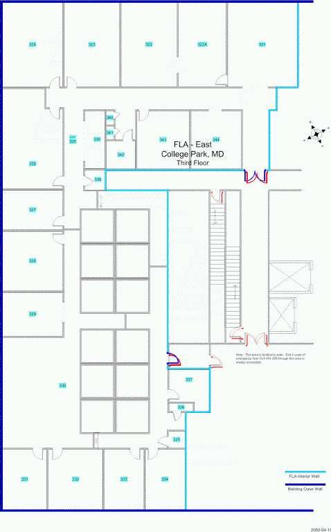
tion errors in the current systems. The Horus system point chooses only the locations in the range of the firstFigure 7: Floor plan for the first testbed. Readings were Figure 8: Floor plan of the office space where the second
collected in the corridors and inside the rooms. experiment was conducted. Readings were collected in
the corridors and inside the rooms.
access point and covered by the second access point and 4.1.1 Testbed 1
so on, leading to a multi-level clustering process.
We performed our first experiment in the south wing of
Notice that no preprocessing is required in the offline the fourth floor of the A. V. Williams building in the Uni-
training phase. During the online phase, a location x be- versity of Maryland at College Park. The layout of the
longs to a cluster whose key is access point a if there floor is shown in Figure 7. The wing has a dimension of
is information about access point a at location x in the 68.2 meters by 25.9 meters. The technique was tested
radio map. in the University of Maryland wireless network using
The algorithm works as follows. Given a sequence of Cisco access points. 21 access points cover the multi-
observations from each access point, we start by sort- story wing and were involved in testing.
ing the access points in descending order according to The radio map has 110 locations along the corridors
the average received signal strength. For the first access and 62 locations inside the rooms. On the average, each
point, the one with the strongest average signal strength, location is covered by 6 access points. The Horus system
we calculate the probability of each location in the radio was running under the Windows XP professional operat-
map set given the observation sequence from this access ing system.
point alone. This gives us a set of candidate locations 4.1.2 Testbed 2
(locations that have non-zero probability). If the prob-
ability of the most probable location is “significantly” We performed the second experiment in another office
higher (according to a threshold) than the probability of space (Figure 8). The area of the experiment site is ap-
the second most probable location, we return that most proximately 11.8 meters by 35.9 meters covering corri-
probable location as our location estimate, after consult- dors, cubicles, and rooms. Five LinkSys access points
ing only one access point. If this is not the case, we go to and one Cisco access point cover the test area.
the next access point in the sorted access point list. For We have a total of 110 locations in the radio map. On
this access point, we repeat the same process again, but the average, each location is covered by 4 access points.
only for the set of candidate locations obtained from the The Horus system was running under the Linux (kernel
first access point. We study the performance of the IT 2.5.7) operating system.
approach in Section 4. 4.1.3 Data collection
The radio map locations were marked on the floor before
4 Experimental Evaluation the experiment and the user clicked on the map to point
the location of the radio map points. We collected 100
In this section we start by showing the effect of each samples, spaced 300 ms apart, at each radio map loca-
module independently on the the accuracy of the basic tion. We expect an error of about 15-20 cm due to the
algorithm. We then show the effect of using all the com- inaccuracies in clicking the map.
ponents together on the performance of the Horus sys- The training data was placed 1.52 meters (5 feet) apart
tem. for the first testbed and 2.13 meters apart for the second
testbed (7 feet).
4.1 Experimental Testbed For each testbed, we selected 100 test locations to ran-
dom cover the entire test area (none of them coincide
We performed our experiment in two different testbeds. with a training point). For both testbeds, the test set was1
Table 1: Summary of the percentage enhancement of dif-
0.9
ferent components on the basic algorithm
0.8 Technique Testbed 1 Testbed 2
0.7 Correlation Handling 19% 11%
0.6 Center of Mass 13% 6%
Probability
0.5 Time Averaging 24% 15%
0.4 Small-Scale Compensator 25% 21%
0.3
0.2 0.8
Average distance error (Meter)
0.1 Non-Parametric 0.7
Parametric
0
0 1 2 3 4 5 6 0.6
Distance Error (Meter)
0.5
Figure 9: Performance of the basic algorithm of the Ho- 0.4
rus system for the first testbed. 0.3
0.2
0.1 Without Corr.
collected by different persons on different days and times With Corr.
of day than the training set. This difference presents 0
1 2 3 4 5
a realistic testbed and should, if anything, decrease the
Number of samples (n)
measured accuracy of our approach because it lessens
the likelihood that the test data is a close match to the
Figure 10: Average distance error with and without tak-
training data.
ing correlation into account for the first testbed.
4.2 Results
We show the effect of each module independently on the
performance of the discrete-space estimator and present averaged samples increases, the performance degrades.
the overall system performance in Section 4.3. The minimum value at n = 2 can be explained by noting
4.2.1 Discrete-space estimator (Basic algorithm) that there are two opposing factors affecting the system
accuracy:
Figure 9 shows the performance of the basic algorithms
of the Horus system for the first testbed. The system 1. as the number of averaged samples n increases, the
can achieve an accuracy of 1.4 meters 90% of the time. accuracy of the system should increase.
The performance of the parametric and non-parametric
methods is comparable with a slight advantage for the 2. as n increases, the estimation of the distribution of
parametric method. Using a parametric distribution to the average of the n samples becomes worse due to
estimate the signal-strength distribution smooths the dis- the wrong independence assumption.
tribution shape to account for missing signal strength val-
ues in the training phase (due to the finite training time). At low values of n (n = 1, 2) the first factor is the dom-
This smoothing avoids obtaining a zero probability for inating factor and hence the accuracy increases. Start-
any signal strength value that was not obtained in the ing from n = 3, the effect of the bad estimation of the
training phase and hence enhances the accuracy. distribution becomes the dominating factor and accuracy
Table 1 shows the summary of the results for the two degrades.
testbeds. Details for the second testbed can be found in Using the modified technique, the system average ac-
[28]. curacy is enhanced by more than 19% using five signal-
strength samples.
4.2.2 Correlation handler
4.2.3 Continuous space estimator
Figure 10 shows the performance of the Horus system
when taking the correlation into account and without tak- Center of Mass Technique: Figure 11 shows the effect of
ing the correlation into account for the first testbed. We increasing the parameter N (number of locations to in-
estimated the value of α to be 0.9. The figures show that terpolate between) on the performance of the center of
under the independence assumption, as the number of mass technique for the first testbed. Note that the specialAverage distance error (Meter) 0.7 0.7
Average Distance Error (Meter)
0.6 0.6
0.5 0.5
0.7
0.4 0.6 0.4
0.5
0.3 0.4 0.3
0.3
0.2 0.2 0.2
0.1
0.1 0 0.1
0 2 4 6 8 10
0 0
0 20 40 60 80 100 120 140 160 180 0 0.02 0.04 0.06 0.08 0.1 0.12 0.14 0.16 0.18 0.2
Number of locations (N) Perturbation Fraction
Figure 11: Average distance error using the center of Figure 13: Effect of changing the perturbation fraction
mass technique for the first testbed. on average distance error.
0.7 each access point) on average error. We can see from this
Average distance error (Meter)
0.6 figure that the best value for the perturbation fraction is
0.05 for the first testbed. We use these values for the rest
0.5 of this section.
0.4
Figure 14 shows the effect of increasing the number
of perturbed access points on the average distance error.
0.3 The access points chosen at a location are the strongest
access points in the set of access points that cover that
0.2
location. The figure shows that perturbation technique is
0.1 not sensitive to the number of access points. This means
that perturbing one access point only is sufficient to en-
0
0 2 4 6 8 10 hance the performance.
Averaging window size (W)
Figures 15 shows the effect of using the perturbation
technique on the basic Horus system. The perturbation
Figure 12: Average distance error using the time- technique reduces the average distance error by more
averaging technique for the first testbed. than 25% and the worst-case error is reduced by more
than 30%.
4.2.5 Clustering module
case of N = 1 is equivalent to the discrete-space estima- Figures 16 and 17 shows the effect of the parameter
tor output. The figures show that the performance of the T hreshold on the performance. For small values of the
Horus system is enhanced by more than 13% for N = 6. T hreshold parameter, the decision is taken quickly af-
Time-averaging Technique: Figure 12 shows the ef- ter examining a small number of access points. As the
fect of increasing the parameter W (size of the averag- threshold value increases, more access points are con-
ing window) on the performance of the time-averaging sulted to reach a decision. As the number of access points
technique. The figures show that the larger the averag- consulted increases, the number of operations (multipli-
ing window, the better the accuracy. The performance cations) per location estimate increases and so does the
of the Horus system is enhanced by more than 24% for accuracy.
W = 10.
4.3 Overall System Performance
4.2.4 Small-scale compensator
In the previous sections, we studied the effect of each
For the purpose of detecting small-scale variations, we component of the Horus system separately on the perfor-
assume a maximum user speed of two meters per second. mance. In this section, we compare the performance of
Figure 13 shows the effect of changing the perturba- the full Horus system, to the performance of a determin-
tion fraction (d, which is the amount by which to perturb istic technique (the Radar system [5]) and a probabilisticAverage Distance Error (Meter) 0.5 0.7
Average distance error (Meter)
0.45
0.6
0.4
0.35 0.5
0.3 0.4
0.25
0.2 0.3
0.15 0.2
0.1
0.1
0.05
0 0
1 2 3 No Clust. 0.1 0.3 0.5 0.7
Number of Access Points Used Threshold
Figure 14: Effect of changing the number of perturbed Figure 16: Effect of the parameter T hreshold on the
access points on average distance error. average distance error for the first testbed.
1
0.9 Table 2: Estimation parameters for the two testbeds
0.8 Parameter Test. 1 Test. 2
0.7 Correlation Degree (α) 0.9 0.7
Probability
0.6 Num. of avg. samples (n) 10 10
0.5 Num. of loc. used in interp. (N ) 6 6
0.4 Averaging window (W ) 10 10
0.3 Threshold 0.1 0.1
0.2
0.1 Perturbation
Basic
0 posed techniques.
0 2 4 6
Error Distance (Meter) The performance of the three systems is better in the
first testbed than the second testbed as the first testbed
Figure 15: CDF for the distance error for the first testbed. has a higher density of APs per location and the calibra-
tion points were closer for the first testbed.
Moreover, the Horus system leads to more than an
technique [21]. We use the parametric distribution tech- order of magnitude savings in the number of multipli-
nique. Table 2 shows the values of different parameters. cations required per location estimate compared to the
other systems (250 multiplications for Horus compared
Figures 18 shows the comparison for the two testbeds to 2708 for the other two systems).
(the curve for the Radar system is truncated). Tables 3 We also applied the enhancement discussed in this pa-
summarizes the results. The table shows that the average per (without correlation handling) to the Radar system.
accuracy of the Horus system is better than the Radar We summarize the results is Table 3. These results show
system by more than 89% for the first testbed and 82% the effectiveness of the techniques proposed in the paper
for the second testbed. The worst case error is decreased and that these techniques are general and can be applied
by more than 93% for the first testbed and 70% for the to other WLAN location determination systems to en-
second testbed. hance their accuracy.
Comparing the probabilistic system in [21] to the Ho-
rus system shows that the average error is decreased by
more than 35% for the first testbed and 27% for the sec- 5 Discussion
ond testbed. The worst case error is decreased by more
than 78% for the first testbed and 70% for the second In this section, we highlight some of our experience with
testbed. These results show the effectiveness of the pro- the Horus system.Table 3: Comparison of the Horus system and other systems (error in centimeters)
Testbed 1 Testbed 2
Median Avg Stdev 90% Max Median Avg Stdev 90% Max
Horus 39 42 28 86 121 51 64 53 132 289
System [21] 48 65 63 143 578 72 86 77 181 991
Radar 296 400 326 853 1757 341 361 184 611 967
Radar with Horus tech. 161 193 107 302 423 142 195 106 332 483
is dependent on the application in use.
Avg. num. of oper. per location estimate
4000
80 Latency can be reduced by presenting the location es-
3500 70 timate incrementally using one sample at a time. The
60
3000 50 system need not to wait until it acquires the n samples
40 all at once. Instead, it can give a more accurate estimate
2500 30
20 of the location as more samples become available by re-
2000 10 porting the estimated location given the partial samples
0
1500 0.1 0.3 0.5 0.7 it has. Other factors that affect the choice of the value of
n are the user mobility rate and the sampling rate. The
1000
higher the user mobility rate or the sampling rate, the
500 lower the value of n.
0 5.3 User Profile
No Clust. 0.1 0.3 0.5 0.7
Threshold A common assumption of WLAN location determination
systems is that the user position follows a uniform distri-
Figure 17: Effect of the parameter T hreshold on the bution over the set of possible locations. Our analysis
average number of operations per location estimate for and experimentation [32] show that knowing the prob-
the first testbed. The sub-figure shows the same curve ability distribution of the user position can reduce the
for T hreshold = [0.1, 0.7]. number of access points required to obtain a given accu-
racy. However, with a high density of access points, the
performance of the Horus system is consistent under dif-
ferent probability distributions for the user position, i.e.,
5.1 Parametric vs Non-Parametric Distri- the effect of the user profile is not significant with a high
butions density of access points. Systems can use this fact to re-
duce the energy consumed in the location determination
The Horus system can model the signal strength distribu-
algorithm by not using the user profile in the estimation
tions received from the access points using parametric or
process.
non-parametric distributions. The main advantage of the
non-parametric technique is the efficiency of calculating 5.4 Effect of Different Hardware
the location estimate, while the parametric technique re- One of the hardware related questions is whether differ-
duces the radio map size and smooths the distribution ent hardware from different manufacturers are compati-
shape which leads to a slight computational advantage of ble. That is, how does using different APs, mobile de-
the parametric technique over the non-parametric tech- vices, or wireless cards affect the accuracy?
nique. Our experience with the Horus system shows that the
Laptop or PDA used for the calibration has no effect on
5.2 Location Estimation Latency
the accuracy if a different device is used in tracking. APs
The correlation handling and the continuous space es- from different manufacturers can be used without affect-
timator modules each use more than one sample to in- ing the accuracy since the radio map captures the sig-
crease the accuracy of the system. However, a side effect nature of the AP at each location (note that the second
of this increased accuracy is that the latency of calculat- testbed uses mixed types of APs). The 802.11h specifica-
ing the location estimate increases. In general, we have a tions, however, require APs to have transmission power
tradeoff between the accuracy required and the latency of control (TPC) and dynamic frequency selection (DFS).
the location estimate. The higher the required accuracy, This presents an open research direction for the current
the higher the number of samples required and the higher WLAN location determination systems as they assume
the latency to obtain the location estimate. This decision that the AP transmission power does not change over1 drivers that support that interface. Under the Windows
OS, NDIS allowed us to perform the same functions.
Our experience with both systems shows that drivers
0.8
under Linux conform to the Wireless Extensions APIs
better than Windows Drivers do with the NDIS. For ex-
Probability
0.6 ample, under the Windows, some cards, like the Cisco
card, respond to scans with low frequency (every 2-3
0.4 seconds) and return only one AP. We hope that future
versions of the driver will have better support for the
0.2 NDIS interface. Moreover for both systems, better ac-
Horus
System [21] tive scanning techniques needs to be developed to reduce
Radar the scanning overhead.
0
0 1 2 3 4 5
Error Distance (Meter) 6 Related Work
(a) First testbed Many systems over the years have tackled the problem
of determining and tracking the user position. Examples
1
include GPS [11], wide-area cellular-based systems [24],
infrared-based systems [4, 26], ultrasonic-based sys-
0.8 tems [19], various computer vision systems [16], and
physical contact systems [18].
Probability
0.6 Compared with these systems, WLAN location de-
termination systems are software based (do not require
0.4 specialized hardware) and may provide more ubiquitous
coverage. This feature adds to the value of the wireless
0.2 data network.
Horus
System [21] The Daedalus project [14] developed a system for
Radar coarse-grained user location. A mobile host estimates
0
0 1 2 3 4 5 its location to be the same as the base station to which
Error Distance (Meter) it is attached. Therefore, the accuracy of the system is
(b) Second testbed
limited by the access point density.
The RADAR system [5] uses the RF signal strength
Figure 18: CDF of the performance of the Horus system as an indication of the distance between the transmitter
and the Radar and the probabilistic system. and receiver. During an offline phase, the system builds
a radio map for the RF signal strength from a fixed num-
ber of receivers. During normal operation, the RF signal
strength of the mobile client is measured by a set of fixed
time. receivers and is sent to a central controller. The central
The main factor that may affect the accuracy when controller uses a K-nearest approach to determine the lo-
changing hardware is the wireless card. Our experience cation from the radio map that best fits the collected sig-
shows that cards from the same manufacture are inter- nal strength information.
changeable. The good news is that a linear mapping ex- The Aura system proposed in [22] uses two tech-
ists between different NICs [13]. Unfortunately, some of niques: pattern matching (PM) and triangulation, map-
the cards in the market are so noisy [27] that with this ping and interpolation (TMI). The PM approach is very
linear mapping the obtained radio map is not represen- similar to the RADAR approach. In the TMI technique,
tative of the environment. We found that Orinoco cards the physical position of all the access points in the area
and Cisco cards are stable, in terms of signal-strength needs to be known and a function is required to map sig-
measurements. nal strength onto distances. They generate a set of train-
ing points at each trained position. The interpolation of
5.5 Operating System Interface the training data allows the algorithm to use less training
We implemented the Horus system under both Linux data than the PM approach. During the online phase, they
and Windows. The main functionality we require from use the approximate function they got from the training
the OS is support for issuing scan requests and return- data to generate contours and they calculate the intersec-
ing the results. Under the Linux OS, the wireless exten- tion between different contours yielding the signal space
sions [1,2] give us a common interface to query different position of the user. The nearest set of mappings fromthe signal-space to the physical space is found by apply- handling small-scale variations. The perturbation tech-
ing a weighted average, based on proximity, to the signal nique enhances the average distance error by more than
space position. 25% for the first testbed and more than 21% for the sec-
The Nibble location system, from UCLA, uses a ond testbed. Moreover, the worst-case error is reduced
Bayesian network to infer a user location [8]. Their by more than 30% for the two testbeds.
Bayesian network model include nodes for location, The basic Horus technique chooses the estimated lo-
noise, and access points (sensors). The signal to noise cation from the discrete set of radio map locations. We
ratio observed from an access point at a given location described two techniques for allowing continuous-space
is taken as an indication of that location. The system estimation: the Center of Mass technique and the Time-
also quantizes the SNR into four levels: high, medium, Averaging technique. Using the Center of Mass tech-
low, and none. The system stores the joint distribution nique, the accuracy of the Horus system was increased
between all the random variables of the system. by more than 13% for the first testbed and by more than
Another system, [21], uses Bayesian inversion to re- 6% for the second testbed compared to the basic tech-
turn the location that maximizes the probability of the re- nique. The Time-Averaging technique enhances the per-
ceived signal strength vector. The system stores the sig- formance of the Horus system by more than 24% for the
nal strength histograms in the radio map and uses them first testbed and more than 15% for the second testbed.
in the online phase to estimate the user location. Yet, The two techniques are independent and can be applied
another system, [17], applies the same technique to the together.
robotics domain. We also compared the performance of the Horus sys-
The Horus system is unique in defining the possible tem to the performance of the Radar system. We showed
causes of variations in the received signal strength vec- that the average accuracy of the Horus system is better
tor and devising techniques to overcome them, namely than the Radar system by more than 89% for the first
providing the correlation modeler, correlation handler, testbed and 82% for the second testbed. The worst case
continuous space estimator, and small-space compen- error is decreased by more than 93% for the first testbed
sator modules. Moreover, it reduces the computational and 70% for the second testbed. Comparing the prob-
requirements of the location determination algorithm by abilistic system in [21] to the Horus system shows that
applying location-clustering techniques. This allows the the average error is decreased by more than 35% for the
Horus system to achieve its goals of high accuracy and first testbed and 27% for the second testbed. The worst
low energy consumption. case error is decreased by more than 78% for the first
testbed and 70% for the second testbed. These results
7 Conclusions show the effectiveness of the proposed techniques. In
In this paper, we presented the design of the Horus terms of computational requirements, the Horus system
system: a WLAN-based location determination system. is more efficient by more than an order of magnitude.
We approached the problem by identifying the various The proposed modules are all applicable to any of
causes of variations in a wireless channel and developed the current WLAN location determination systems. We
techniques to overcome them. We also showed the vari- show the result of applying the techniques of the Horus
ous components of the system and how they interact. system to the Radar system. The results show that the
The Horus system models the signal strength distribu- average distance error is reduced by more than 58% for
tions received from access points using parametric and the first testbed and by more than 54% for the second
non-parametric distributions. By exploiting the distribu- testbed. The worst case error is decreased by more than
tions, the Horus system reduces the effect of temporal 76% for the first testbed and by more than 48% for the
variations. second testbed.
We showed that the correlation of the samples from As part of our ongoing work we are experimenting
the same access point can be as high as 0.9. Experi- with different clustering techniques. Automating the
ments showed that under the independence assumption, radio-map generation process is a possible research area.
as the number of averaged samples increases, the per- The Horus system provides an API for location-aware
formance degrades. Therefore, we introduced the cor- applications and services. We are looking at designing
relation modeler and handling modules that use an au- and developing applications and services over the Horus
toregressive model for handling the correlation between system. A possible future extension is to dynamically
samples from the same access point. Using the modi- change the system parameters based on the environment,
fied technique, the system average accuracy is enhanced such as changing the averaging window size as the user
by more than 19% for the first testbed and 11% for the speed changes or using a time-dependent radio map. We
second testbed. are also working on the theoretical analysis of different
The Horus system uses the Perturbation technique for components of the system.Our experience with the Horus system showed that it [13] H AEBERLEN , A., F LANNERY, E., L ADD , A., RUDYS , A.,
WALLACH , D., AND K AVRAKI , L. Practical Robust Localiza-
has achieved its goals of: tion over Large-Scale 802.11 Wireless Networks. In 10th ACM
MOBICOM (Philadelphia, PA, September 2004).
• High accuracy: through a probabilistic location de- [14] H ODES , T. D., K ATZ , R. H., S CHREIBER , E. S., AND ROWE ,
L. Composable ad hoc mobile services for universal interaction.
termination technique, using a continuous-space es- In 3rd ACM MOBICOM (September 1997), pp. 1–12.
timator, handling the high correlation between sam- [15] K RISHNAN , P., K RISHNAKUMAR , A., J U , W. H., M ALLOWS ,
C., AND G ANU , S. A System for LEASE: Location Estima-
ples from the same access point, and the perturba- tion Assisted by Stationary Emitters for Indoor RF Wireless Net-
tion technique to handle small-scale variations. works. In IEEE Infocom (March 2004).
[16] K RUMM , J., ET AL . Multi-camera multi-person tracking for Easy
Living. In 3rd IEEE Int’l Workshop on Visual Surveillance (Pis-
• Low computational requirements: through the use cataway, NJ, 2000), pp. 3–10.
[17] L ADD , A. M., B EKRIS , K., RUDYS , A., M ARCEAU , G.,
of clustering techniques. K AVRAKI , L. E., AND WALLACH , D. S. Robotics-Based Lo-
cation Sensing using Wireless Ethernet. In 8th ACM MOBICOM
(Atlanta, GA, September 2002).
The design of Horus also allows it to achieve scalabil- [18] O RR , R. J., AND A BOWD , G. D. The Smart Floor: A Mech-
ity to large coverage areas, through the use of clustering anism for Natural User Identification and Tracking. In Confer-
ence on Human Factors in Computing Systems (CHI 2000) (The
techniques, and to large number of users, through the dis- Hague, Netherlands, April 2000), pp. 1–6.
tributed implementation on the mobile devices and due to [19] P RIYANTHA , N. B., C HAKRABORTY, A., AND BALAKRISH -
NAN , H. The Cricket Location-Support system. In 6th ACM
the low energy requirements of the algorithms. MOBICOM (Boston, MA, August 2000).
Moreover, the techniques presented in this paper may [20] ROOS , T., M YLLYMAKI , P., AND T IRRI , H. A Statistical Mod-
eling Approach to Location Estimation. IEEE Transactions on
be applicable to other RF-technologies such as 802.11a, Mobile Computing 1, 1 (January-March 2002), 59–69.
802.11g, HiperLAN, and BlueTooth. [21] ROOS , T., M YLLYMAKI , P., T IRRI , H., M ISIKANGAS , P., AND
S IEVANEN , J. A Probabilistic Approach to WLAN User Loca-
tion Estimation. International Journal of Wireless Information
Acknowledgments Networks 9, 3 (July 2002).
[22] S MAILAGIC , A., S IEWIOREK , D. P., A NHALT, J., KOGAN , D.,
AND WANG , Y. Location Sensing and Privacy in a Context Aware
This work was supported in part by the Maryland In- Computing Environment. Pervasive Computing (2001).
formation and Network Dynamics (MIND) Laboratory, [23] S TALLINGS , W. Wireless Communications and Networks,
first ed. Prentice Hall, 2002.
its founding partner Fujitsu Laboratories of America, [24] T EKINAY, S. Special issue on Wireless Geolocation Systems and
and by the Department of Defense through a University Services. IEEE Communications Magazine (April 1998).
[25] T HE I NSTITUTE OF E LECTRICAL AND E LECTRONICS E NGI -
of Maryland Institute for Advanced Computer Studies NEERS , I NC . IEEE Standard 802.11 - Wireless LAN Medium
Access Control (MAC) and Physical Layer (PHY) specifications.
(UMIACS) contract. [26] WANT, R., H OPPER , A., FALCO , V., AND G IBBONS , J. The Ac-
tive Badge Location System. ACM Transactions on Information
Systems 10, 1 (January 1992), 91–102.
Availability [27] Y EO , J., BANERJEE , S., AND AGRAWALA , A. Measuring traffic
on the wireless medium: experience and pitfalls. In Technical Re-
The MAPI API and the Linux device drivers are available port, CS-TR 4421, Department of Computer Science, University
for download at [1]. of Maryland, College Park (Dec. 2002).
[28] YOUSSEF, M. Horus: A WLAN-Based Indoor Location Deter-
mination System. PhD thesis, University of Maryland at College
References Park, May 2004. Submitted for SigMobile Dissertation Page.
[29] YOUSSEF, M., A BDALLAH , M., AND AGRAWALA , A. Mul-
[1] http://www.cs.umd.edu/users/moustafa/Downloads.htm. tivariate Analysis for Probabilistic WLAN Location Determina-
[2] http://www.hpl.hp.com/personal/Jean Tourrilhes/. tion Systems. In The Second Annual International Conference on
[3] http://www.orinocowireless.com. Mobile and Ubiquitous Systems: Networking and Services (July
[4] A ZUMA , R. Tracking requirements for augmented reality. Com- 2005).
munications of the ACM 36, 7 (July 1997). [30] YOUSSEF, M., AND AGRAWALA , A. Small-Scale Compensation
[5] BAHL , P., AND PADMANABHAN , V. N. RADAR: An In- for WLAN Location Determination Systems. In IEEE WCNC
Building RF-based User Location and Tracking System. In IEEE 2003 (March 2003).
Infocom 2000 (March 2000), vol. 2, pp. 775–784. [31] YOUSSEF, M., AND AGRAWALA , A. Handling Samples Corre-
[6] BAHL , P., PADMANABHAN , V. N., AND BALACHANDRAN , A. lation in the Horus System. In IEEE Infocom (March 2004).
Enhancements to the RADAR User Location and Tracking Sys- [32] YOUSSEF, M., AND AGRAWALA , A. On the Optimality of
tem. Tech. Rep. MSR-TR-00-12, Microsoft Research, February WLAN Location Determination Systems. In Communication
2000. Networks and Distributed Systems Modeling and Simulation
[7] B OX , G. E. P., J ENKINS , G. M., AND R EINSEL , G. C. Time Conference (January 2004).
Series Analysis: Forcasting and Control, third ed. Prentice Hall, [33] YOUSSEF, M., AGRAWALA , A., AND S HANKAR , A. U. WLAN
1994. Location Determination via Clustering and Probability Distribu-
[8] C ASTRO , P., C HIU , P., K REMENEK , T., AND M UNTZ , R. A tions. In IEEE PerCom 2003 (March 2003).
Probabilistic Location Service for Wireless Network Environ- [34] YOUSSEF, M., AGRAWALA , A., S HANKAR , A. U., AND N OH ,
ments. Ubiquitous Computing 2001 (September 2001). S. H. A Probabilistic Clustering-Based Indoor Location Deter-
[9] C ASTRO , P., AND M UNTZ , R. Managing Context for Smart mination System. Tech. Rep. UMIACS-TR 2002-30 and CS-
Spaces. IEEE Personal Communications (OCTOBER 2000). TR 4350, University of Maryland, College Park, March 2002.
[10] C HEN , G., AND KOTZ , D. A Survey of Context-Aware Mobile http://www.cs.umd.edu/Library/TRs/.
Computing Research. Tech. Rep. Dartmouth Computer Science
Technical Report TR2000-381, 2000.
[11] E NGE , P., AND M ISRA , P. Special issue on GPS: The Global
Positioning System. Proceedings of the IEEE (January 1999),
3–172. Notes
[12] G WON , Y., JAIN , R., AND K AWAHARA , T. Robust Indoor Loca- 1 The normalization is used to ensure that the sum of the probabili-
tion Estimation of Stationary and Mobile Users. In IEEE Infocom ties of all locations equals one.
(March 2004).You can also read