A Novel Decentralized Game-Theoretic Adaptive Traffic Signal Controller: Large-Scale Testing - MDPI
←
→
Page content transcription
If your browser does not render page correctly, please read the page content below
sensors
Article
A Novel Decentralized Game-Theoretic Adaptive
Traffic Signal Controller: Large-Scale Testing
Hossam M. Abdelghaffar 1,2 and Hesham A. Rakha 3, *
 1    Department of Computers & Control Systems, Engineering Faculty, Mansoura University, Mansoura,
      Dakahlia 35516, Egypt; hossamvt@vt.edu
 2    Center for Sustainable Mobility, Virginia Tech Transportation Institute, Virginia Tech,
      Blacksburg, VA 24061, USA
 3    Charles E. Via, Jr. Dept. of Civil and Environmental Engineering, Director of the Center of Sustainable
      Mobility, Virginia Tech Transportation Institute, Virginia Tech, Blacksburg, VA 24061, USA
 *    Correspondence: hrakha@vt.edu

 Received: 26 March 2019; Accepted: 13 May 2019; Published: 17 May 2019

 Abstract: This paper presents a novel de-centralized flexible phasing scheme, cycle-free, adaptive
 traffic signal controller using a Nash bargaining game-theoretic framework. The Nash bargaining
 algorithm optimizes the traffic signal timings at each signalized intersection by modeling each phase
 as a player in a game, where players cooperate to reach a mutually agreeable outcome. The controller
 is implemented and tested in the INTEGRATION microscopic traffic assignment and simulation
 software, comparing its performance to that of a traditional decentralized adaptive cycle length and
 phase split traffic signal controller and a centralized fully-coordinated adaptive phase split, cycle
 length, and offset optimization controller. The comparisons are conducted in the town of Blacksburg,
 Virginia (38 traffic signalized intersections) and in downtown Los Angeles, California (457 signalized
 intersections). The results for the downtown Blacksburg evaluation show significant network-wide
 efficiency improvements. Specifically, there is a 23.6% reduction in travel time, a 37.6% reduction
 in queue lengths, and a 10.4% reduction in CO2 emissions relative to traditional adaptive traffic
 signal controllers. In addition, the testing on the downtown Los Angeles network produces a 35.1%
 reduction in travel time on the intersection approaches, a 54.7% reduction in queue lengths, and a 10%
 reduction in CO2 emissions compared to traditional adaptive traffic signal controllers. The results
 demonstrate significant potential benefits of using the proposed controller over other state-of-the-art
 centralized and de-centralized adaptive traffic signal controllers on large-scale networks both during
 uncongested and congested conditions.

 Keywords: traffic signal control; game theory; decentralized control; large-scale network control

1. Introduction
     Traffic growth and limited available capacity within the roadway system produces problems
and challenges for transportation agencies. Traffic congestion affects traveler mobility and has an
impact on air quality, and consequently on public health. The stopping and starting in traffic jams
burns fuel at a higher rate than the smooth rate of travel, and contributes to the amount of emissions
released by vehicles that create air pollution and are related to global warming [1]. Reduction in traffic
congestion improves traveler mobility and accessibility, while also reducing vehicle fuel consumption
and emissions.
     Traffic congestion in 2013 cost Americans $124.2 billion [2], and this number is projected to rise to
$186.2 billion in 2030. Traffic signal controllers attempt to optimize various traffic variables (e.g., delay,
queue length, and energy and emission levels), by optimizing signal control variables, including the
cycle length, the phasing scheme and sequence, the phase split, and the offset. Most of the currently

Sensors 2019, 19, 2282; doi:10.3390/s19102282                                      www.mdpi.com/journal/sensors
Sensors 2019, 19, 2282 2 of 20
implemented traffic signal systems can be categorized into one of the following categories: fixed-time
control (FP), actuated control (ACT), responsive control, or adaptive control [3].
An FP control system is developed off-line using historical traffic data to compute traffic signal
timings; real-time traffic data is not taken into account, and the duration and order of all phases
stay fixed without any adaptation to real-time traffic demand fluctuations [4]. Previous studies
have found this approach to only be appropriate for under-saturated conditions and traffic flows
that are stable or relatively stable [5]. By comparison, ACT systems respond to changes in traffic
demand patterns by communicating with the controller based on the presence or absence of vehicles as
identified by local detectors installed at intersection approach stop lines. While ACT has been proven
to generally perform better than FP for very low demand levels, it still offers no real-time optimization
to adapt to traffic fluctuations, and may result in long network queues [6]. Adaptive systems have
the potential to alleviate traffic congestion by adjusting signal timing parameters in response to
real-time traffic fluctuations. These systems use detector inputs, historical trends, and predictive
models to predict vehicle arrivals at intersections, and then use the predictions to determine the
best gradual changes in cycle length, phase splits, and offsets to minimize vehicle delays or queue
lengths [7]. Some examples in this category are: the Split Cycle Offset Optimization Tool (SCOOT) [8],
a macroscopic model that minimizes delay and the number of vehicle stops at all intersection
approaches, and performs effectively in under-saturated traffic conditions. The Sydney Coordinated
Adaptive Traffic System (SCATS) [9] operates in a centralized hierarchical mode, and allocates green
times to the phases of greatest need. OPAC [10] optimizes an objective function for a specified rolling
horizon using dynamic-programming-based traffic prediction models that require a traffic environment
state transition probability model, which can be difficult to generate. TR2 and UTCS-1 [11], optimized
off-line, are incapable of handling stochastic variations in traffic patterns.
The operation of actuated and adaptive controllers is constrained by minimum and maximum
cycle lengths, green indication durations and offsets, and also require going through a pre-defined
sequence of phases. In addition, some systems use hierarchies that either partially or totally centralize
decisions, rendering them more susceptible to failures. Hierarchies make scaling these systems up
more difficult, relatively more complex to operate, and more expensive [12].
Various computational intelligence-based techniques have been investigated in the domain
of traffic signal optimization domain, and are still under continuous research and development,
using fuzzy sets, genetic algorithms, reinforcement learning, and neural networks. Genetic algorithms
compute the optimal solution using an evolutionary process of possible solutions [13,14]; it solves
simple networks and deals with static traffic volumes. However, as the network increases in size,
the search space involved in finding effective signal plans increases significantly, and a large amount of
centralized computing power is required. Pappis [15] proposed the first signal controller using fuzzy
logic for an isolated intersection. Ella [16] proposed a neuro-fuzzy controller, where the parameters of
the fuzzy membership functions were adjusted using a neural network. The neural learning algorithm
in Ella’s work was reinforcement learning, which was found to be successful at constant traffic volumes,
but failed when the traffic demand changed rapidly. The choice of the membership functions (building
blocks of fuzzy set theory) are important for a particular problem since they affect a fuzzy inference
system. As a traffic control system is a complex large-scale system with many interactive factors, it is
more appropriate to use fuzzy control for isolated intersections [17].
Several approaches have been proposed for designing traffic signal controllers using neural
networks [18,19]. Most of these works are based on a distributed approach, where an agent is assigned
to update the traffic signals of a single intersection. Neural networks also adapt very slowly to
changing traffic parameters, where on-line learning has to take place continuously. Some networks
require multiple models to be maintained for various times within a day. Most intelligence-based
approaches are still being researched and are thus under development or have only been implemented
and tested on an isolated intersection, so their effectiveness for controlling a large-scale traffic network
is also unknown.Sensors 2019, 19, 2282 3 of 20
Reinforcement learning is inspired by behavioral psychology [20]. It is a machine learning
approach which allows agents to interact with the environment, attempting to learn the optimal
behavior based on the feedback received from interactions. The feedback may be available right
after the action, or several time steps later, which makes the learning more challenging [21].
Abdulhai et al. [22] applied a model-free Q-learning technique to a simple two-phase isolated traffic
signal in a two-dimensional road network. Salkham et al. [23] applied a Q-learning strategy that
allowed an agent to exchange rewards with its neighbors on 64 signalized intersections. The state-action
space was simple and very time coarse. Each agent decided the phase splits every two cycles, which did
not capture of the rapid dynamics of congestion–coordination between the agents actions was missing.
Studies have considered the use of RL algorithms for traffic control, but they are very limited in
terms of network complexity and traffic loadings, so that realistic scenarios, over saturated conditions,
and transitions from under saturation to over saturation (and vice versa) have not been fully explored.
Game theory studies the interactive cooperation between intelligent rational decision makers
with the specific goal of cooperating and benefiting from reaching a mutually agreeable outcome.
It has been widely used in economic, military, communication applications [24,25], model traveler
route choice behavior [26], control connected vehicle movements [27], and to in-route guidance [28].
The literature indicates that investigation of game-theoretic traffic signal control is very limited.
Bargaining theory is related to cooperative games through the concept of Nash bargaining (NB).
A bargaining situation is defined as a situation in which multiple players with specific objectives
cooperate and benefit by reaching a mutually agreeable outcome [29]. The bargaining process is the
procedure that bargainers follow to reach an agreement (outcome) [30], and the bargaining outcome is
the result of the bargaining process [31,32].
Traffic flow is affected by a number of factors, including weather, time-of-day, day-of-week,
and unpredictable events, such as special events, incidents, and work zones. Consequently,
traffic control strategies could be improved if control systems responded not only to actual conditions,
but also adapted their actions to transient conditions. Due to the stochastic nature of traffic flows,
an adaptive control strategy that adjusts to stochastic changes is needed. Cycle-free strategies may
present an innovative and less restrictive means of accommodating variations in traffic conditions.
Traffic signal controllers can be categorized as centralized or decentralized. Centralized
systems require a reliable and direct communication network between a central computer and
the local controllers. The main advantage of these systems is that they allow for traffic signal
coordination. However, decentralized systems offer many advantages over centralized control systems
as they are computationally less demanding and require only relevant information from adjacent
intersections/controllers. Robustness is also guaranteed in decentralized control systems, because if
one or more controllers fail, the remaining controllers can take over some of their tasks. Decentralized
systems are scalable and easy to expand by inserting new controllers into the system. Additionally,
decentralized systems are often inexpensive to establish and operate, as there is no essential need for a
reliable and direct communication network between a central computer and the local controllers in
the field.
To mitigate traffic congestion, a novel de-centralized traffic signal controller, considering a flexible
phasing sequence and cycle-free operation, using a NB game-theoretic framework (DNB) is developed.
The proposed controller was implemented and evaluated in the INTEGRATION microscopic traffic
assignment and simulation software [33–35]. INTEGRATION is a microsopic model that replicates
vehicle longitudinal motion using the Rakha–Pasumarthy–Adjerid collision-free car-following model,
also known as the RPA model [36]. The RPA model captures vehicle steady-state car-following behavior
using the Van Aerde model [37,38]. Movement from one steady state to another is constrained by a
vehicle dynamics model described in [39,40]. Vehicle lateral motion is modeled using lane-changing
models described in [35]. The model estimates of vehicle delay were validated in [41], while vehicle stop
estimation procedures are described and validated in [42]. Vehicle fuel consumption and emissions
are modeled using the VT-Micro model [43–45]. The developed controller was compared to theSensors 2019, 19, 2282 4 of 20
operation of a decentralized phase split and cycle length controller (PSC) [6], and a fully coordinated
adaptive phase split-cycle length and offset optimization controller (PSCO) to evaluate its performance,
where PSCO is based on the REALTRAN (REAL-time TRANsyt) controller that emulates the SCOOT
system [46,47]. The DNB controller was implemented and evaluated on large-scale networks consisting
of 38 (Blacksburg) and 457 (downtown Los Angeles) signalized intersections.
This paper describes the application and the testing of the proposed DNB controller on large-scale
networks and is organized as follows. Section 2 describes the developed de-centralized traffic signal
controller using a game-theoretic framework. Section 3 presents the experimental setup and results
of a large-scale study in the town of Blacksburg, Virginia, consisting of 38 signalized intersections.
Section 4 describes the experimental setup and the experimental results of a large-scale study on a
downtown network in Los Angeles, California, consisting of 457 signalized intersections. Section 5
presents a summary and conclusions drawn from these studies.
2. Traffic Signal Controller
This section describes the NB solution for two players (Section 2.1), Section 2.2 describes how
the NB approach is adapted and extended to control a multi-phase (player) signalized intersection
(DNB), and Section 2.3 describes the de-centralized mechanism of the DNB controller over an entire
transportation network.
2.1. NB Solution for Two Players
A bargaining situation is defined as a situation in which multiple players with specific objectives
cooperate and benefit by reaching a mutually agreeable outcome (agreement). In bargaining theory,
there are two concepts: the bargaining process and the bargaining outcome.
The bargaining process is the procedure that bargainers follow to reach an agreement (outcome).
Nash adopted an axiomatic approach that abstracts the bargaining process and considers only the
bargaining outcome [31]. The bargaining problem consists of three basic elements: players, strategies,
and utilities (rewards). Bargaining between two players is illustrated in the bi-matrix shown in Table 1.
Each player, namely P1 and P2 , has a set of possible actions A1 and A2 , whose outcome preferences are
given by the utility functions u and v, respectively, as they take relevant actions.
Table 1. Two players matrix game.
P2
A1 A2
A1 u1 , v1 u2 , v2
P1
A2 u3 , v3 u4 , v4
The space (S) shown in Figure 1, is the set of all possible utilities that the two players can achieve;
the vertices of the area are the utilities where each player chooses their pure strategy. The disagreement
or the threat point d = (d1 , d2 ) corresponds to the minimum utilities that the players want to achieve.
The threat point is a benchmark, and its selection affects the bargaining solution. Each player attempts
to choose their threat point in order to maximize their bargaining position. Subsequently, a bargaining
problem is defined as the pair (S,d) where S ∈ R2 and d ∈ S such that S is a convex and compact set,
and there exists some s ∈ S such that s > d.
Nash’s theorem states that there exist a unique solution satisfying four axioms (Pareto efficiency,
symmetry, invariance to equivalent utility representation, and independence of irrelevant alternatives),
and this solution is the pair of utilities (u∗ , v∗ ) that solves the following optimization problem:
max (u − d1 )(v − d2 )
u,v
(1)
s.t.(u, v) ∈ S, (u, v) ≥ (d1 , d2 )Sensors 2019, 19, 2282 5 of 20
The NB solution (u∗ , v∗ ) of this optimization problem can be calculated as the point in the
bargaining set that maximizes the product of the players utility gains relative to a fixed threat point.
Figure 1. Utility region.
2.2. DNB Traffic Signal Controller for Multi-Players
This section describes the game model and the DNB solution for multi-players (N), and shows how
the model is adapted (from Section 2.1) and applied to control a multi-phase signalized intersection.
First, a four-phase scheme for a four-legged intersection is used, assuming four players (N = 4),
to represent the intersection phases as shown in Figure 2, with protected, leading main street
left-turn phases.
Figure 2. Phasing scheme.
In the game model, the four phases are modeled as four players P1 , P2 , P3 , and P4 in a four-player
cooperative game. For each player (phase), there are two possible actions: maintain ( A1 ) or change
( A2 ). These actions produce the state for the traffic signal. Specifically, the action maintain maintains
the traffic signal (i.e., if it is displaying a green indication, it will remain green; if it is displaying a
red indication, it will remain red). The action change entails changing the state of the traffic signal
(i.e., if it is displaying a green indication, it will switch its state by first introducing a yellow indication
followed by a red indication; if it is red, it will switch to a green indication) in the simulated time
interval. The combinations of phases offer four possibilities, where only one player holds the green
indication and all others hold red indications [48].
The INTEGRATION software is a microscopic traffic simulation model that traces individual
vehicle movements every deci-second. Driver characteristics such as reaction times, acceleration and
deceleration levels, desired speeds, and lane-changing behavior are examples of stochastic variables
that are modeled in INTEGRATION. The threshold speed is fixed and assigned to the entire network
(chosen to be equal to the typical pedestrian speed, s Th = 4.5 (km/h)). We continuously check the
vehicle speeds when they are within the threat distance from the approach stop bar. If the vehicle (v)
speed (stv ) is less than the threshold speed (s Th ) at time (t), the vehicle is assigned to the queue, and the
current queue length associated with the corresponding lane (l) is updated. Once the vehicle’s speed
exceeds (s Th ) the queue length is updated (i.e., shortened by the number of vehicles leaving the queue).
This is formulated mathematically as
qtl = ∑ qtv (2)
v∈vtlSensors 2019, 19, 2282 6 of 20
if stv−1 > s Th & stv ≤ s Th
1
−1 t −1 Th t Th
( sv ≤ s & sv > s
if
qtv = (3)
if stv−1 ≤ s Th & stv ≤ s Th
0
if stv−1 > s Th & stv > s Th
qtl is the number of queued vehicles in lane l at time t. The index (t − 1) is used to refer to the previous
time step. In this case the previous deci-second as the INTEGRATION model tracks vehicle movements
at a frequency of 10 hertz.
The utilities (rewards) for each player (phase) in the game can be defined as the estimated sum
of the queue lengths in each phase after applying a specific action. The estimated queue length after
applying a specific action is calculated according to the following equation:
Q P (t + ∆t) = ∑ qtl + Qinl ∆t − Qoutl ∆t (4)
l∈P
where ∆t is the updating time interval, qtl is the current queue length at time t, Q P (t + ∆t) is the
estimated queue length after ∆t for phase P, Qinl is the arrival flow rate (veh/h/lane), and Qoutl is the
departure flow rate (veh/h/lane).
The NB solution is extended to four players (N=4) with a four-dimensional utility space and
threat points. The solution for the four-phase NB problem can be formulated as:
N
max ∏ ( ui − di )
(u1 ,...,u N i =1
) (5)
s.t.(u1 , ..., uN ) ∈ S, (u1 , ..., uN ) ≥ (d1 , ..., dN )
The NB solution can be calculated as the vector that maximizes the product of the player’s utility
gains relative to a fixed threat point. The threat point represents the maximum number of vehicles
that could be accumulated per lane (i.e., the maximum measurable queue length). The objective is to
minimize and equalize the queue lengths across the different phases. Hence, the negative queue length
is used as the utility of each strategy considering a negative threat point. In other words, the reward
(u) is defined to be the negative of the estimated queue length (Q P ), i.e., u = − Q P , and we substitute
(d) with a negative number. Consequently, the objective function can be rewritten as follows:
N
max ∏ (di − QPi )
( Q P1 ,...,Q PN i =1
) (6)
s.t.(QP1 , ..., QPN ) ∈ S, (QP1 , ..., QPN ) ≤ (d1 , ..., dN )
The block diagram for the DNB controller is shown in Figure 3, where the predefined threat point
values are an input to the controller (i.e., the maximum queue size that each player can accommodate).
Qoutl are generally measured at the approach stop bar, whereas Qinl are measured at a distance from
the stop bar equal to the threat point divided by the approach jam density (i.e., the maximum length of
the queue assuming all vehicles are stopped).
Queue Length
Prediction ql , Qinl , Qoutl
QP
Threat
points DNB Signal Timing Traffic
Controller Environment
Measurements
sv , G, R
Figure 3. System block diagram.Sensors 2019, 19, 2282 7 of 20
The flows Qinl and Qoutl can be measured using stationary sensors (e.g., loop detectors or through
video image processor (VIP) detection obtained from CCTV cameras). The queue length estimates can
be obtained using CCTV cameras or via GPS-equipped vehicles that communicate with the the traffic
signal controller. As such, the proposed controller is technology agnostic.
2.3. DNB Controller for Multi-Intersections
This section presents the DNB controller formulation for a network composed of multiple
signalized intersections. For illustration purposes only, we formulate the problem considering three
signalized intersections, as shown in Table 2. It should be noted, however that the algorithm can
operate on a network of any number of signalized intersections.
Assume we have three signalized intersections (I1 , I2 , I3 ), each traffic signal has three phases
(Ph1 , Ph2 , Ph3 ), where each phase is modeled as a player in a game resulting in a total of nine players
where I1 has three players (P1 , P2 , P3 ), I2 has three players (P4 , P5 , P6 ), and I3 has three players
(P7 , P8 , P9 ). Each traffic signal has three possible actions (A), where one phase displays a green
indication (G) while the others display a red indication (R), as illustrated in Table 2.
Table 2. Multi-player matrix game.
Intersection First Intersection (I1 ) Second Intersection (I2 ) Third Intersection (I3 )
Player
Ph1(P1 ) Ph2(P2 ) Ph3(P3 ) Ph1(P4 ) Ph2(P5 ) Ph3(P6 ) Ph1(P7 ) Ph2(P8 ) Ph3(P9 )
Action
G R R G R R G R R
First | {z } | {z } | {z }
A11 A21 A31
R G R R G R R G R
Second | {z } | {z } | {z }
A12 A22 A32
R R G R R G R R G
Third | {z } | {z } | {z }
A13 A23 A33
Consequently, for the three signalized network illustrated in Table 2, there are 27 possible scenarios
(action permutations) as shown in Table 3. The optimum overall network performance (NB optimum,
Equation (6)) can be computed from Table 3.
Referring to Table 2, and assuming that the first traffic signal (I1 ) has action (A12 ) that optimizes
its performance, traffic signal (I2 ) has action (A21 ) that optimizes its performance, and traffic signal
(I3 ) has action (A33 ) that optimizes its performance. Consequently, searching in Table 3 for the Nash
optimum combination yields scenario 12. This implies that in order to achieve the Nash optimum
network performance, it is sufficient to search for the actions that optimize the operations of each
signalized intersection. This can be described using the NB optimization problem shown in the
following equations.
9
max
(u ,...,u )
∏ ( ui − di )
1 9 i =1
3 6 9
= max [∏ (ui − di ) ∏ ( ui − di ) ∏ ( ui − di ) ]
(u1 ,...,u9 ) i =1 i =4 i =7
| {z } | {z } | {z } (7)
I1 I2 I3
3 6 9
= max
(u ,...,u )
∏ ( ui − di ) max
(u ,...,u )
∏ ( ui − di ) max
(u ,...,u )
∏ ( ui − di )
1 3 i =1 4 6 i =4 7 9 i =7
| {z } | {z } | {z }
I1 I2 I3Sensors 2019, 19, 2282 8 of 20
The network-wide Nash optimum solution is obtained by maintaining the Nash optimum
solution at each signalized intersection. As such, while the proposed NB controller is decentralized
(i.e., DNB), it still produces the network-wide Nash-optimum control strategy relying solely on
edge computing. The Nash optimum should not be mistaken for the system-optimum solution,
where the system optimum might sacrifice the performance of one or more traffic signals to achieve
optimum network-wide performance. It should be noted that obtaining the system-optimum solution is
impossible given the scale and level of interactions of the various network-wide traffic signal controllers.
The DNB controller, thus, provides a scalable and resilient controller that circumvents the problems
inherent in complex centralized systems with minimum sacrifices to network-wide performance.
Table 3. All possible Network Actions (Permutations).
Scenario # Network Action
1 A11 A21 A31
2 A11 A21 A32
3 A11 A21 A33
4 A11 A22 A31
5 A11 A22 A32
6 A11 A22 A33
7 A11 A23 A31
8 A11 A23 A32
9 A11 A23 A33
10 A12 A21 A31
11 A12 A21 A32
12 A12 A21 A33
13 A12 A22 A31
14 A12 A22 A32
15 A12 A22 A33
16 A12 A23 A31
17 A12 A23 A32
18 A12 A23 A33
19 A13 A21 A31
20 A13 A21 A32
21 A13 A21 A33
22 A13 A22 A31
23 A13 A22 A32
24 A13 A22 A33
25 A13 A23 A31
26 A13 A23 A32
27 A13 A23 A33
Note that a single traffic signal cannot be decomposed (i.e., optimize each decision variable
independently), as the utilities of the players within the same traffic signal are dependent on each other.
Specifically, if one player displays a green indication by default the other players have to display a
red indication given that this would result in conflicting movements being discharged simultaneously.
Alternatively, each traffic signal controller operates independently. Consequently, decomposition is
invalid within a traffic signal but valid between traffic signals, as players within a traffic signal compete
for the same resource, namely green time.
3. Blacksburg Town Experiments
This section presents the experimental setup and the results of a testing of the proposed system in
the town of Blacksburg, Virginia, illustrated in Figure 4. The simulations were conducted using
the morning peak hour (7–8 a.m.) traffic demand. The town of Blacksburg has 38 signalized
intersections, 549 stop signs, 30 yield signs, and 1844 links. The minimum free-flow speed on
the network was 30 (km/h), and the maximum free-flow speed on the network was 105 (km/h).Sensors 2019, 19, 2282 9 of 20
The minimum link length was 50 m while the maximum link length was 2932 m. The jam density was
set at 160 (veh/km/lane). The traffic signal phasing scheme used in the study was the same as those
in the field. These varied between 2 to 4 phases.
3.1. Blacksburg Experimental Setup
The time-dependent static O-D demand matrices were generated every 15 min using the
QueensOD software [49–51]. QueensOD estimates the most likely O-D matrix that is as close
structurally as a seed matrix while at the same time minimizing the error between the estimated and
field observed link flow counts. The time-dependent static O-Ds were then used to compute a dynamic
O-D matrix using procedures described in [52]. The final peak-hour dynamic O-D matrix consisted
of 23, 260 vehicular trips. Vehicles were loaded for one hour, while the simulation continued until all
vehicles cleared the network to ensure that the same number of vehicles were used in comparing the
performance of the various traffic signal control algorithms.
The performance of the DNB controller was evaluated by comparing its performance to that
of the PSC and PSCO controllers. The network-wide average of each of the following measures of
effectiveness (MOEs) was calculated to assess the DNB controller’s performance: travel time, total
delay, stopped delay, queue length, fuel consumption, and emission levels. The INTEGRATION
microscopic traffic assignment and simulation software was used to model the network, shown in
Figure 4. Three experiments were conducted on the BB network, as discussed in the following sections.
Figure 4. Blacksburg network.
3.2. BB Experimental Results: 1
In this experiment the performance of the DNB controller was compared to the PSC and PSCO
controllers. The threat point (d) values per lane for the DNB controller were assigned based on the
link’s lengths (L), the link’s free-flow speeds (U f ), and the updating time intervals (∆t), using the
following formula; d=min[N ( L/2), N (U f ×∆t)], where N ( L/2) represents the number of vehicles
that could be accumulated up to the half length of the link, and N (U f ×∆t) represents the maximum
number of stopped vehicles that could be stored in the distance (U f × ∆t). Using this distance allowed
vehicles to proceed through the intersection in a minimal time without stopping if there was no queue
ahead of them. A distance of L/2 was used instead of L to get a better estimate of the queue length
for each movement because drivers typically moved to their desired lanes as they got closer to the
signalized intersection, and to avoid being fully queued (i.e., players will accept a fully occupied
(queued) link).
The average MOE values over the entire simulation for the PSC, PSCO, and DNB control scenarios
are summarized in Table 4. In addition, Table 4 shows the percent improvement in MOEs using the
proposed DNB controller over the PSC and PSCO controllers. The improvement (%) is calculated as:
MOE(PSC/PSCO) − MOE(DNB)
Improvement(%) = × 100 (8)
MOE(PSC/PSCO)Sensors 2019, 19, 2282 10 of 20
Table 4. Average measures of effectiveness (MOEs) and (%) improvement for game-theoretic framework
(DNB) DNB over phase split and cycle length controller (PSC) and phase split-cycle length and offset
optimization controller (PSCO) controllers.
System
PSC PSCO DNB
MOE
Average Total Delay (s/veh) 96.234 100.197 80.323
Improvement % 16.534 19.823
Average Stopped Delay (s/veh) 20.285 25.649 12.1074
Improvement % 40.314 52.7962
Average Travel time (s) 306.254 310.225 290.175
Improvement % 5.25 6.46
Average Number of Stops 4.662 4.5899 4.281
Improvement % 8.18 6.734
Average Fuel (L) 0.4142 0.4129 0.40
Improvement % 3.38 3.07
Average CO2 Emissions (g) 913.833 912.495 883.127
Improvement % 3.36 3.22
The simulation results demonstrated a significant reduction in the average travel time of 5.25%,
a reduction in the average total delay of 16.5%, and a reduction in the average stopped delay of
40.3% over the PSC controller. In addition, the results indicated significant reduction in the average
travel time of 6.5%, a reduction in the average total delay of 19.8%, and a reduction in the average
stopped delay of 52.7% over the PSCO controller. These results show that the proposed DNB controller
outperforms both the PSC and PSCO controllers.
3.3. BB Experimental Results: 2
This section presents a potential solution to better estimate the queue length considering the
driver’s lane changing behavior close to the intersections. A suggested phasing scheme, shown in
Figure 5b, where all vehicles on the link discharge in a single phase, might provide a better estimate
of the queue length per phase over the currently implemented phase scheme shown in Figure 5a,
where each link discharges in two phases. Two simulations were conducted using the DNB controller
to evaluate the effectiveness of the two phasing scheme on the MOEs, where the threat point per lane
was assigned using the following formula: d=min[N ( L/2), N (U f × ∆t)]. The simulation results using
the two schemes (Figure 5) are shown in Table 5.
(a) (b)
Figure 5. Four phasing scheme. (a) Implemented phasing scheme. (b) Suggested phasing scheme.
Table 5. MOEs using two different phasing schemes.
System
DNB (Field Scheme) DNB (Modified Scheme ) Imp. (%)
MOE
Average Total Delay (s/veh) 80.323 94.712 −17.913
Average Stopped Delay (s/veh) 12.107 24.381 −101.374
Average Travel Time (s) 290.175 302.425 −4.222
Average Number of Stops 4.281 4.417 −3.177
Average Fuel (L) 0.40 0.41 −2.274
Average CO2 Emissions (g) 883.127 902.277 −2.168Sensors 2019, 19, 2282 11 of 20
The simulation results demonstrate that the suggested phasing scheme does not improve the
network performance.
3.4. BB Experimental Results: 3
This section presents the effect of reducing the number of vehicles that can be accumulated in a
lane on the network’s performance. The minimum free-flow speed on the network was 30 (km/h),
and the maximum free-flow speed on the network was 105 (km/h), with updating time intervals of
10 s. Assigning the detector locations to be the min(L/2, U f × ∆t), the detectors could be located for
long links between 84 m (i.e., 13 veh/lane) to 292 m (i.e., 47 veh/lane). Employing the free-flow speed
to determine the threat point (d = min[N ( L/2), N (U f × ∆t)]) is a good choice for low traffic demand,
as vehicles are not required to stop at the intersection); however, for high traffic demand, long links
can accommodate long queues, which causes delays for the vehicles on that link. Hence, reducing the
number of vehicles that can accumulate in a lane might enhance the network’s performance. To examine
the effectiveness of changing the maximum number of vehicles that could be accumulated per lane
on the MOEs, a sensitivity analysis was conducted, as shown in Figure 6, with d = min[N ( L/2), NV],
where NV presents the maximum number of vehicles that can be stored in a lane; this number ranges
between 6 to 32 vehicles.
Analysis of the results in Figure 6 demonstrated that better performance using the DNB controller
could be achieved if the threat points are assigned as a minimum of 12 veh/lane and the number of
vehicles that could be accumulated in L/2, (d=min[N ( L/2), 12]).
Table 6 shows the average MOEs values over the entire simulation time and the percent
improvement in MOEs using the proposed DNB controller over PSC and PSCO controllers. Simulation
results indicate significant reduction in the average total delay of 19.38%, a reduction in the average
stopped delay of 51.18%, a reduction in the average travel time of 6.162%, a reduction in the average
number of stops of 8.39%, a reduction in the average fuel consumption of 3.89%, and a reduction in the
emission levels of 3.84% over the PSC controller. The results show that the proposed DNB approach
outperforms both the PSC and PSCO controllers.
(a) (b)
Figure 6. Sensitivity analysis. (a) Average travel time. (b) Average CO2 .Sensors 2019, 19, 2282 12 of 20
Table 6. Average MOEs and (%) improvement using DNB over the PSC and PSCO controllers.
System
PSC PSCO DNB
MOE
Average Total Delay (s/veh) 96.234 100.197 77.577
Improvement % 19.3871 22.575
Average Stopped Delay (s/veh) 20.285 25.649 9.903
Improvement % 51.182 61.391
Average Travel Time (s) 306.254 310.225 287.384
Improvement % 6.162 7.362
Average Number of Stops 4.662 4.5899 4.271
Improvement % 8.393 6.95
Average Fuel (L) 0.4142 0.4129 0.3981
Improvement % 3.887 3.584
Average CO2 (grams) 913.833 912.495 878.739
Improvement % 3.84 3.7
To further investigate the achieved improvements using the DNB controller, it was taken into
consideration that the network has 459 stop signs and 30 yield signs, which might conceal the full
degree of improvement achieved using the DNB controller on the signalized intersection. Accordingly,
we investigated the percent improvement in MOEs using the DNB controller over the PSC controller
over only the links that were directly associated with intersections. Table 7 shows the percent
improvement in MOEs using the DNB controller over the PSC controller on the 38 intersections.
Table 7 demonstrates an improvement in the travel time on the intersections between 6% to 52%,
an improvement in the queue length on the intersections between 8% to 60%, and an improvement
in the number of stops on the intersections between 8% to 80%. In addition, Table 7 demonstrates
an overall reduction in the average travel time of 23.63%, in the average queued vehicles of 37.66%,
in the average number of stops of 23.58%, in the average fuel consumption of 10.44%, in the average
CO2 emitted of 9.84%, and in the average NOX emitted of 5.4% over the PSC controller. These results
revealed that the DNB controller performs significantly better than the PSC controller.Sensors 2019, 19, 2282 13 of 20
Table 7. Intersections (%) improvement of MOEs using DNB over PSC controller.
MOEs
Travel Time Queue Num. of Stops CO2 Fuel NOX
Int. #
1 6.15 22.02 24.31 2.65 2.57 0.16
2 16.41 26.80 21.18 7.71 7.71 5.86
3 8.49 18.23 32.78 6.03 6.45 9.04
4 31.11 52.87 39.56 8.17 6.60 8.76
5 22.23 53.88 52.91 9.36 8.96 3.31
6 23.18 34.44 14.24 11.59 10.72 4.75
7 8.97 15.88 17.83 3.89 3.60 2.27
8 24.06 41.87 16.11 13.75 13.48 9.16
9 40.71 56.27 29.85 25.25 24.65 13.84
10 13.40 26.35 41.44 8.63 8.65 9.77
11 17.63 26.34 11.80 9.01 8.35 1.35
12 7.64 7.97 32.65 3.48 3.37 3.48
13 19.41 37.91 20.92 8.99 8.75 3.76
14 28.50 35.50 25.36 7.85 6.62 8.15
15 23.87 39.63 34.58 12.55 12.27 6.17
16 27.55 59.10 41.88 15.11 14.79 8.84
17 42.00 60.00 56.97 16.90 14.83 12.84
18 26.26 49.88 32.72 14.49 13.41 5.70
19 19.68 36.53 21.10 4.96 4.25 4.98
20 52.24 76.08 63.09 32.97 31.76 20.16
21 34.82 50.16 46.27 21.57 21.39 18.27
22 38.27 59.40 37.47 27.63 27.28 26.53
23 17.19 30.86 16.27 7.60 6.92 5.26
24 34.67 44.00 11.27 14.63 13.34 3.24
25 23.48 44.59 57.38 5.76 4.50 0.09
26 18.03 26.03 30.50 4.02 2.48 0.75
27 28.13 36.34 8.57 16.77 16.19 14.48
28 14.53 35.05 11.90 9.46 9.85 11.61
29 13.13 19.12 9.60 5.35 4.99 1.14
30 23.63 47.38 23.22 19.33 19.41 24.77
31 32.76 55.70 80.38 18.00 17.27 19.33
32 34.76 53.07 35.46 26.64 27.05 29.31
33 35.98 48.47 15.26 20.35 19.56 11.67
34 16.68 32.68 30.34 11.27 11.15 11.76
35 18.01 28.95 21.58 18.24 18.67 26.12
36 22.59 46.51 34.33 7.68 7.03 2.47
37 29.31 46.50 31.49 7.40 6.68 1.08
38 14.32 14.55 8.06 4.67 4.17 1.14
Overall (%) 23.63 37.67 23.59 10.44 9.84 5.39
4. Downtown Los Angeles Experiments
This section describes the experimental setup and the experimental results of large scale studies
in downtown Los Angeles, California comprised of 457 signalized intersections.
4.1. Los Angeles Experimental Setup
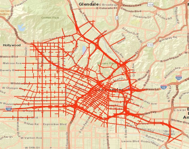
These experiments were large scale studies of a network in downtown Los Angeles (LA),
California, including the most congested downtown area, as shown in Figure 7a. The INTEGRATION
microscopic traffic assignment and simulation software was used to model the network, as shown
in Figure 7b.
Simulations were conducted using the morning peak hour (7–8 a.m.) traffic demand that was
calibrated in a previous effort [53]. The downtown LA network has 457 signalized intersections,
285 stop signs, 23 yield signs, and 3556 links. The origin-destination (O-D) demand matrices
were generated, as described earlier, using a combination of the QueensOD software, to generate
time-dependent static O-D demands, and then converting these static O-D demands to a dynamic O-DSensors 2019, 19, 2282 14 of 20
demand. The resulting O-D consisted of a total of 143,957 vehicle trips. Vehicles were loaded for the
one-hour period and the simulation continued until all vehicles cleared the network to ensure that all
comparisons were made for the same number of vehicles.
The traffic signal phasing schemes varied from 2 to 6 phases, reflecting the field implemented
traffic signal settings in downtown LA. The minimum free-flow speed on the network was 15 (km/h),
and the maximum free-flow speed on the network was 120 (km/h). The minimum link length on the
network was 50 m, and the maximum link length on the network was 4400 m. The jam density of the
various network links was set equal to 180 (veh/km/lane).
(a) (b)
Figure 7. Downtown Los Angeles network. (a) LA, Google maps. (b) LA, INTEGRATION.
The DNB controller was compared to the PSC controller to evaluate their relative performance.
The average of each of the following measures of effectiveness (MOEs) was calculated to assess
the performance of the DNB controller: travel time, total delay, stopped delay, queue length,
fuel consumption, and emission levels.
4.2. LA Experimental Results: 1
In this experiment, the performance of the DNB controller was compared to that of the PSC
controller using the full traffic demand in the morning peak hour. The threat point per lane for the
DNB controller was assigned as the minimum of 12 veh/lane and the number of vehicles that could be
accumulated on L/2 (i.e., d = min[N ( L/2), 12]) based on the sensitivity analysis shown in Figure 8.
(a) (b)
Figure 8. LA Sensitivity Analysis. (a) Average Travel Time. (b) Average Fuel Consumption.
The average MOE values over the entire simulation for the PSC and DNB controllers are shown
in Table 8. In addition, Table 8 shows the percent improvement in MOEs using the proposed DNB
controller relative to the PSC controller. The simulation results demonstrate a significant reductionSensors 2019, 19, 2282 15 of 20
in the average the average travel time of 7.89%, a reduction in the total delay of 14.55%, a reduction
in the average stopped delay of 25.18%, a reduction in the average number of vehicle stops of 12.4%,
a reduction in the average fuel consumption of 4.0%, and a reduction in CO2 emission levels of 4.25%,
relative to the PSC controller. Analysis of the results demonstrated that the proposed DNB controller
outperforms current state-of-the-art de-centralized traffic signal controllers.
Table 8. Average MOEs and the (%) improvement using DNB controller over PSC controller (100% Demand).
System
PSC DNB DNB Imp. (%)
MOE
Average Total Delay (s/veh) 557.46 476.35 14.55
Average Stopped Delay (s/veh) 256.77 192.12 25.18
Average Travel Time (s) 1034.27 952.73 7.89
Average Number of Stops 7.41 6.49 12.40
Average Fuel (L) 1.16 1.11 4.00
Average CO2 (grams) 2482.13 2376.59 4.25
The improvements produced by the DNB controller, only at the signalized intersections,
were further analyzed. Accordingly, we investigated the percent improvement in MOEs using the
DNB controller over the PSC controller over only the links that were directly associated with signalized
intersections. Table 9.
Table 9 demonstrates a reduction in the average travel time of 35.16%, a reduction in the average
queued vehicles of 54.67%, a reduction in the average number of stops of 44.03%, a reduction in the
average fuel consumption of 9.97%, a reduction in the CO2 emissions of 9.92%, and a reduction in the
NOX emissions of 11.78% relative to the PSC controller. These results revealed that the DNB controller
has significantly better performance potential than the PSC controller.
Table 9. Average (%) improvements of MOEs using DNB controller over PSC controller (100% Demand),
over the links that are directly associated with intersections.
MOEs
Travel Time Queue Num. of Stops CO2 Fuel NOX
Int. #
Overall 457 Int. (%) 35.16 54.66 44.03 9.97 9.92 11.77
4.3. LA Experimental Results: 2
A simulation was conducted for lower levels of traffic congestion by scaling the demand down by
90% (i.e., 10% of the peak demand) to investigate the performance potential using the DNB controller.
Table 10 shows a reduction in the average travel time of 7.1%, a reduction in the average total delay
of 36.79%, a reduction in the average stopped delay of 90.26%, a reduction in the average number of
vehicle stops of 34.66%, a reduction in the average fuel consumption of 4.8%, and a reduction in CO2
emission levels of 4.79%, relative to the PSC controller.
Table 10. Average MOEs and the (%) improvement using DNB over PSC controller (10% Demand).
System
PSC DNB DNB Imp. (%)
MOE
Average Total Delay (s/veh) 84.94 53.69 36.79
Average Stopped Delay (s/veh) 19.97 1.95 90.26
Average Travel Time (s) 450.11 418.18 7.10
Average Number of Stops 4.48 2.92 34.66
Average Fuel (L) 0.85 0.81 4.80
Average CO2 (grams) 1830.27 1742.53 4.79
Once more, to further investigate the achieved improvements using the DNB controller,
we investigated the improvement in MOEs over only the links that were directly associated withSensors 2019, 19, 2282 16 of 20
signalized intersections, as shown in Table 11. Table 11 demonstrates a reduction in the average travel
time of 19.19%, a reduction in the average queued vehicles of 49.84%, a reduction in the average
number of stops of 53.71%, a reduction in the average fuel consumption of 54.16%, a reduction in
the average CO2 emitted of 16.09%, and a reduction in the average NOX emitted of 25.94% over
PSC controller.
These results demonstrate that the DNB controller performed significantly better than the PSC
controller in both congested and uncongested conditions, however, produced more savings as the
traffic demand decreased.
Table 11. Average (%) improvements of MOEs using DNB over PSC controller (10% Demand) over the
links directly associated with intersections.
MOEs
Travel Time Queue Num. of Stops CO2 Fuel NOX
Int. #
Overall 457 Int. (%) 19.19 49.84 53.71 54.16 16.09 25.94
The results show that the DNB controller yielded significant improvements in the average values
of all MOEs, demonstrating improved system efficiency.
5. Summary & Conclusions
The research presented in this paper develops and evaluates a Nash bargaining de-centralized
flexible phasing cycle-free traffic signal controller (DNB controller) on large-scale networks.
The controller was implemented and tested in the INTEGRATION microscopic traffic assignment
and simulation software. The performance of the DNB controller was compared to a decentralized
phase split and cycle length optimization controller based on the HCM procedures (PSC) and a
fully-coordinated adaptive phase split, cycle length and offset optimization controller (PSCO), in the
town of Blacksburg, Virginia and in downtown Los Angeles, California.
Several simulations were conducted on the Blacksburg network using different threat point values
and phasing schemes to determine their effect on the controller’s performance. The results show
significant reductions in the network-wide average travel time of 6.1% and 7.3%, a reduction in the
average total delay of 19.3% and 22.6%, a reduction in the stopped delay of 51% and 61%, and a
reduction in CO2 emission levels of 3.8% and 3.7%, over the PSC and PSCO controllers, respectively.
In addition, the results show significant reductions on the intersection approach average travel time of
23.6%, a reduction in the average queue length of 37.6%, a reduction in the average number of vehicle
stops of 23.6%, a reduction in the fuel consumption of 9.8%, a reduction in the CO2 emissions of 10.4%,
and a reduction in NOX emissions of 5.4%.
In addition, the DNB controller’s performance was tested in downtown Los Angeles, California,
and compared to the performance of the de-centralized PSC controller. The results show significant
improvements in various network-wide measures of performance. Specifically, a reduction in the
average travel time of 8%, a reduction in the average total delay of 14.5%, a reduction in the stopped
delay of 25.1%, a reduction in the average number of vehicle stops of 12.4%, and a reduction in CO2
emissions of 4.25%, over the PSC controller. Moreover, the results show significant improvements in
the signalized intersection operations with a reduction in the average travel time of 35.1%, a reduction
in the average queue length of 54.7%, a reduction in the average number of vehicle stops of 44%,
a reduction in the fuel consumption and CO2 emissions of 10%, and a reduction in NOX emissions
of 11.7%. Furthermore, simulations conducted for lower traffic demand levels showed significant
network-wide improvements with a reduction in the average total delay of 36.7%, a reduction in the
stopped delay of 90.2%, and a reduction in the average number of stops of 35% over the PSC controller.
As these results indicate, the DNB controller can generate major performance improvements at lower
demands. The results demonstrate significant potential benefits of using the proposed controller over
other state-of-the-art centralized and de-centralized controllers on large scale networks.Sensors 2019, 19, 2282 17 of 20
In summary, a novel traffic signal controller is developed that offers a number of unique features.
First, the controller adapts signal timings dynamically to changing traffic conditions without using
historical data, which tends to be inaccurate, resulting in inefficient traffic signal plans. Second,
the developed controller is de-centralized, which increases both the scalability and robustness of the
system, to avoid the problems inherent with complex centralized communication. Decentralized
systems are often inexpensive to establish and operate, as there is no essential need for a reliable and
direct communication network between a central computer and the local controllers in the field. Third,
the controller, while de-centralized, does not sacrifice in system-wide performance and computes the
network-wide Nash optimum solution. Finally, the controller is designed to operate with current traffic
signal controllers. This controller should increase the traffic handling capacity of roads, and reduce
unnecessary stop-and-go vehicular movement, which will reduce fuel consumption and, accordingly,
air pollution.
Author Contributions: The work described in this article is the collaborative development of all authors,
conceptualization, H.M.A. and H.A.R; methodology, H.M.A. and H.A.R.; software, H.M.A. and H.A.R.; validation,
H.M.A. and H.A.R.; formal analysis, H.M.A. and H.A.R.; investigation, H.M.A. and H.A.R.; writing—review and
editing, H.M.A. and H.A.R.
Funding: This effort was funded by the US Department of Transportation through the University Mobility and
Equity Center (Award 69A3551747123).
Conflicts of Interest: The authors declare no conflicts of interest.
References
1. Elbakary, M.I.; Abdelghaffar, H.M.; Afrifa, K.; Rakha, H.A.; Cetin, M.; Iftekharuddin, K.M. Aerosol
Detection Using Lidar-Based Atmospheric Profiling. In SPIE Optics and Photonics for Information Processing
XI; SPIE: Bellingham, WA, USA, 2017; doi:10.1117/12.2275626.
2. The future economic and environmental costs of gridlock in 2030; Technical Report; Center for Economics and
Business Research: London, UK, 2014.
3. Dai, Y.; Zhao, D.; Zhang, Z. Computational Intelligence in Urban Traffic Signal Control: A Survey.
IEEE Trans. Syst. Man, Cybern. 2012, 42, 485–494, doi:10.1109/TSMCC.2011.2161577. [CrossRef]
4. Turky, A.M.; Ahmad, M.S.; Yusoff, M.; Hammad, B.T. Using genetic algorithm for traffic light control
system with a pedestrian crossing. In Proceedings of the 4th International Conference, RSKT, Gold Coast,
Australia, 14–16 July 2009; doi:10.1007/978-3-642-02962-2_65.
5. Yang, X. Comparison Among Computer Packages in Providing Timing Plans for Iowa Arterial in Lawrence,
Kansas. J. Transp. Eng. 2001, 127, 311–318, doi:10.1061/(ASCE)0733-947X(2001)127:4(311). [CrossRef]
6. Roess, R.; Prassas, E.S.; McShane, W.R. Traffic Engineering, 4th ed.; Pearson Higher Education, Inc.:
Upper Saddle River, NJ, USA, 2010.
7. French, L.J.; French, M.S. Benefits of Signal Timing Optimization and ITS to Corridor Operations; Technical
Report; French Engineering, LLC: Spring, TX, USA, 2006.
8. Hunt, P.B.; Robertson, D.I.; Bretherton, R.D.; Winton, R.I. SCOOT-A Traffic Responsive Method of Coordinating
Signals; Technical Report; Transport and Road Research Laboratory: Wokingham, UK, 1981.
9. Sims, A.G.; Dobinson, K.W. SCAT-The Sydney Co-ordinated Adaptive Traffic System Philosophy and
Benefits. In Proceedings of the International Symposium on Traffic Control Systems, Berkeley, CA,
USA, 6–9 August 1979.
10. Gartner, N.H. OPAC: A demand-responsive strategy for traffic signal control. Transp. Res. Rec. J. Transp.
Res. Board 1983, 906, 75–81.
11. MacGowan, J.; Fullerton, I.J. Development and testing of advanced control strategies in the urban traffic
control system. Public Roads 1979, 43, 97–105.
12. Evans, M.R. Balancing Safety and Capacity in an Adaptive Signal Control System—Phase 1; Technical Report
FHWA-HRT-10-038; Federal Highway Administration: Washington, DC, USA, 2010.
13. Ceylan, H.; Bell, M.G.H. Traffic signal timing optimization based on genetic algorithm approach, including
driver’s routing. Transp. Res. Part B 2004, 38, 329–342, doi:10.1016/S0191-2615(03)00015-8. [CrossRef]Sensors 2019, 19, 2282 18 of 20
14. Chin, Y.; Yong, K.; Bolong, N.; Yang, S.; Teo, K. Multiple Intersections Traffic Signal Timing Optimization
with Genetic Algorithm. In Proceedings of the IEEE International Conference on Control System,
Computing and Engineering, Penang, Malaysia, 25–27 November 2011; doi:10.1109/ICCSCE.2011.6190569.
15. Pappis, C.; Mamdani, E. A Fuzzy Logic Controller for a Traffic Junction Systems. IEEE Trans. Man Cybern.
1977, 7, 707–717, doi:10.1109/TSMC.1977.4309605. [CrossRef]
16. Bingham, E. Neurofuzzy Traffic Signal Control; Helsinki University of Technology: Espoo, Finland, 1998.
17. Liu, Z. A Survey of Intelligence Methods in Urban Traffic Signal Control. Int. J. Comput. Sci. Netw. Secur.
2007, 7, 105–112.
18. Spall, J.; Chin, D. A model-free approach to optimal signal light timing for system-wide traffic control.
In Proceedings of the 33rd IEEE Conference on Decision and Control, Lake Buena Vista, FL, USA, 14–16
December 1994; doi:10.1109/CDC.1994.411110.
19. Srinivasan, D.; Choy, M.C.; Cheu, R.L. Neural Networks for Real-Time Traffic Signal Control. IEEE Trans.
Intell. Transp. Syst. 2006, 7, 261–272, doi:0.1109/TITS.2006.874716. [CrossRef]
20. Shoham, Y.; Powers, R.; Grenager, T. Multi-Agent Reinforcement Learning: A Critical Survey; Technical
Report; Computer Science Department, Stanford University: Stanford, CA, USA, 2003.
21. Sutton, R.S.; Barto, A.G. Reinforcement Learning: An Introduction; The MIT Press: Cambridge, MA, USA;
London, UK, 2012.
22. Abdulhai, B.; Pringle, R.; Karakoulas, G.J. Reinforcement learning for true adaptive traffic signal control.
J. Transp. Eng. 2003, 129, 278–285, doi:10.1061/(ASCE)0733-947X(2003)129:3(278). [CrossRef]
23. Salkham, A.; Cunningham, R.; Garg, A.; Cahill, V. A collaborative reinforcement learning approach to
urban traffic control optimization. In Proceedings of the International Conference on Web Intelligence and
Intelligent Agent Technology, Sydney, Australia, 9–12 December 2008; doi:10.1109/WIIAT.2008.88.
24. Park, H.; van, M. Bargaining strategies for networked multimedia resource management. IEEE Trans.
Signal Process 2007, 55, 3496–3511, doi:10.1109/TSP.2007.893755. [CrossRef]
25. Han, Z.; Liu, K.J.R. Fair Multiuser Channel Allocation for OFDMA Networks Using Nash Bargaining
Solutions and Coalitions. IEEE Trans. Commun. 2005, 53, 1366–1376, doi:10.1109/TCOMM.2005.852826.
[CrossRef]
26. Chen, J. Game-Theoretic Formulations Of Interaction Between Dynamic Traffic Control and Dynamic
Traffic Assignment. Transp. Res. Rec. 1998, 1617, 179–188, doi:10.3141/1617-25. [CrossRef]
27. Elhenawy, M.; Elbery, A.A.; Hassan, A.A.; Rakha, H.A. An Intersection Game-Theory-Based Traffic Control
Algorithm in a Connected Vehicle Environment. In Proceedings of the 2015 IEEE 18th International
Conference on Intelligent Transportation Systems, Las Palmas, Spain, 15–18 September 2015; pp. 343–347,
doi:10.1109/ITSC.2015.65. [CrossRef]
28. Jun, L. Study on Game-Theory-Based Integration Model for Traffic Control and Route Guidance; Tian Jin
University: Tianjin, China, 2003.
29. Abdelghaffar, H.M.; Yang, H.; Rakha, H.A. Isolated Traffic Signal Control using Nash Bargaining
Optimization. Glob. J. Res. Eng. B Automot. Eng. 2016, 16, 27–36.
30. Abdelghaffar, H.M.; Yang, H.; Rakha, H.A. Isolated traffic signal control using a game theoretic framework.
In Proceedings of the IEEE 19th International Conference on Intelligent Transportation Systems (ITSC),
Rio de Janeiro, Brazil, 1–4 November 2016; pp. 1496–1501, doi:10.1109/ITSC.2016.7795755. [CrossRef]
31. Han, Z.; Niyato, D.; Saad, W.; Basar, T.; Hjorungnes, A. Game Theory in Wireless and Communication Networks:
Theory, Models, and Applications; Cambridge University Press: New York, NY, USA, 2012.
32. Abdelghaffar, H.M.; Yang, H.; Rakha, H.A. A Novel Game Theoretic De-Centralized Traffic Signal
Controller: Model Development and Testing. In Proceedings of the 97th Annual Meeting of Transportation
Research Board, Washington, DC, USA, 7–11 January 2018.
33. Aerde, M.V.; Rakha, H.A. INTEGRATION c Release 2.40 for Windows: User’s Guide—Volume I: Fundamental
Model Features; Technical Report; Center for Sustainable Mobility, Virginia Tech Transportation Institute:
Blacksburg, VA, USA, 2012.
34. Aerde, M.V.; Rakha, H.A. INTEGRATION c Release 2.40 for Windows: User’s Guide—Volume II: Advanced
Model Features; Technical Report, Center for Sustainable Mobility, Virginia Tech Transportation Institute:
Blacksburg, VA, 24060, USA, 2013.You can also read