Exploring countrywide spatial systems: 084 SSS10 Proceedings of the 10th International Space Syntax Symposium
←
→
Page content transcription
If your browser does not render page correctly, please read the page content below
SSS10 Proceedings of the 10th International Space Syntax Symposium

084
Exploring countrywide spatial systems:
Spatio-structural correlates at the regional and national scales

Miguel Serra
Space Syntax Laboratory, The Bartlett School of Architecture, University College London.
m.serra@ucl.ac.uk

Bill Hillier
Space Syntax Laboratory, The Bartlett School of Architecture, University College London.
b.hillier@ucl.ac.uk

Kayvan Karimi
Space Syntax Laboratory, The Bartlett School of Architecture, University College London.
k.karimi@ucl.ac.uk

Abstract
In this paper we take a step towards extending space syntax analysis into the countrywide scale,
through the study of three very-large spatial systems in the UK, namely the top-tier road network of
the entire country (170,007 nodes), the complete road network (1,208,674 nodes) of three
contiguous NUTS1 regions (the East of England, South East of England and Greater London) and the
complete road network of UK’s mainland (2,031,971 nodes). We compare the results of our analysis
with several types of functional and socio-economic data, finding clear statistical associations at the
scale of the entire country between network structure, vehicular movement flows and the spatial
distribution of several socio-economic variables. We conclude by arguing that space syntax models
and analysis hold their value at very-large territorial scales, being highly robust and producing
coherent results between datasets of different sources, themes and dimensionalities.

Keywords
Space syntax, territorial scale, regional, national.

1. Introduction
Throughout the last three decades, space syntax has imposed itself as a reliable analytical technique
for quantifying specific structural properties of urban spatial networks, which have been shown to
be strongly associated with a wide range of urban social and functional phenomena. The findings of
the space syntax research programme led to the progressive construction of a new morphological
theory of the city: one that merges objective observational knowledge of urban spatial structures,
with knowledge of the human sociological and behavioural phenomena occurring therein, while
trying to find systematic relations between both; and so, a theory that was able to propose cogent
causal explanations for the fact of cities being like they are (Hillier 1999a, Hillier 2012).

M Serra, B Hillier & K Karimi                                                                             84:1
Exploring countrywide spatial systems: Spatio-structural correlates at the regional and national scales
SSS10 Proceedings of the 10th International Space Syntax Symposium

Space syntax studies have been predominantly dedicated to the inner urban scale - territorial scales
beyond that of the city have been seldom explored. However, the urban phenomenon is today no
longer local, but regional – large contemporary cities are diffuse structures with illusive limits,
frequently encompassing previously separated settlements and former rural hinterlands, within
which fast and little-understood urbanization dynamics take place. Furthermore, spatial networks
are not restricted to the urban environment, either on its historical or contemporary manifestations:
they have always been the vascular systems of human territorial occupancy, extending themselves
between cities, linking them, irrigating and making accessible the entire territory of countries and
beyond. And thus, in view of space syntax’s previous achievements, it seems not too overstated to
say that if its descriptive and predictive capabilities could to be extended to the scale of entire
countries (or even beyond), new insights into human geographic phenomena would be at hand.

In this paper we take a step in that direction, extending space syntax analysis to the countrywide
scale, through the comparison of the analytical results of three large spatial network models, with
several types of functional and socio-economic data. Our aim is to answer the following question: “Is
country-sized space syntax analysis viable?”

By ‘viable’, we mean several things. Firstly, the feasibility of the construction of such large spatial
network models; secondly, the problems raised by their processing time, or even if they are at all
processable by current micro-computers; and thirdly, if space syntax’ analytical results are
meaningful at such large territorial scales; that is, if the patterns revealed by space syntax’ topo-
geometric centrality metrics at the scale of entire countries, show significant statistical associations
with other types of quantified human geographical phenomena, observed at the same territorial
scale.

The rationale behind the expectation that such associations should occur at spatial scales above the
urban, and even at the scale of entire countries and beyond, is straightforward. The development of
space syntax’s topo-geometric centrality measures was the product of previous findings, regarding
particular geometric regularities of urban grids, seemingly universal and systematized formally by
the first time in (Hillier, 1999b). Such regularities pertain to the acknowledgment that all urban
spatial systems, as morphologically diverse as they may seem at first sight, all share the same basic,
underlying dual geometric scheme: a foreground network of main streets - made up of longer street
segments, connected at wide obtuse angles, and thus forming a system of straighter paths - imposed
over a background network of secondary streets – made up of a much greater number of shorter
street segments, connected at nearly right angles; see (Hillier 2012) for a recent recension on this
subject, and on its association with social and economic mechanisms. Even though this basic dual
structuring of urban space has been identified initially in axial maps, the development of segment
models and of the geometric-weighted centrality measures they allow [see (Hillier and Iida 2005) for
details], has made it much easier to detect, visualize and study, because the measures themselves
are sensitive to that particular topo-geometric structuring.

Now, recent findings are making increasingly evident that road networks show geometric and
topological self-similar characteristics, not only at the inner urban scale but also at scales well above
that one (Batty 2005, 2008; Kalapala et al. 2006; Reis 2008; Zhang and Li 2012). We follow this lead,
departing from the simple hypothesis that the foreground/background network principle – that is,
the geometric hierarchization of main paths through their higher linearity regarding secondary paths
- is liable of being extended to territorial scales above that of the city; and, consequently, that space
syntax’s topo-geometric algorithms are bounded to hold their validity at those scales.

One word on the fundamental difference between causality and correlation (i.e. statistical
association) is due, though. It will never be enough to remember that correlation is not causation.
Throughout this work we will be looking at correlations between space syntax centrality measures
and a number of socio-economic phenomena. However, we do not claim direct causal relationships
between the centrality structures thus detected and the spatial distributions of such phenomena –
given the exploratory character of the work that would be unwary, to say the least. But we do claim
that the presence of such statistical associations makes the centrality patterns of countrywide spatial
networks, as described by space syntax measures, reliable proxies of those socio-economic

M Serra, B Hillier & K Karimi                                                                             84:2
Exploring countrywide spatial systems: Spatio-structural correlates at the regional and national scales
SSS10 Proceedings of the 10th International Space Syntax Symposium

phenomena and of their spatial distributions; and that the study of such centrality patterns may
therefore help to clarify how human geographical phenomena are territorialized at the scale of
entire countries.

We start by describing the models, datasets and methods used in this study. We then report the
results of our analysis, showing clear statistical associations between network structure, global
vehicular movement flows and the spatial distribution of several socio-economic variables (namely:
poverty and affluence, the several domains of the UK’s Index of Multi Deprivation, and employment
location). We conclude by arguing that space syntax models and analysis hold their value at very-
large territorial scales, being highly robust and producing coherent results between datasets of
different sources, themes and dimensionalities.

2. Datasets and methods
The bulk of this work was carried out using two different segment models, derived from road-centre
line data (Figure 1). One, representing the system of UK’s A-roads, covering the entire country, with
170,007 nodes and a total road-length of 77,718 Km; and another, covering the Great South-East
(GSE) area of the UK, representing every street segment, with 1,342,365 nodes and a total road-
length of 20,377Km. The A-road’s model (and, later, also the complete UK’s road network model; see
below) were constructed with data from the Meridian2 dataset 1 , and the GSE model was
constructed with data from the Integrated Transport Network (ITN) dataset 2, both provided by UK’s
Ordnance Survey.

The results of the analysis of these two models, and their crossing with several other types of
empirical data, shown that they produced consistent results from a given spatial scale up, but also
that at short spatial scales only complete street network models (as the GSE model) were capable of
emulating certain types of empirical data. Therefore, a last model of the complete road network of
UK’s mainland, with 2,031,971 nodes and a total road-length of 568,333Km, was constructed and
tested through a short analytical exercise, reported in the last section of this paper. However, work
with this very large model is still on-going, and the results shown here are preliminary. The
acknowledgment that the GIS network representation of road-centre lines, when analysed by space
syntax topo-geometric centrality metrics, could emulate the syntactic segment representation
derived from axial lines (Turner 2007), has greatly facilitated the creation of very large spatial
network models. Indeed, today, given the widespread availability of road-centre line data, both from
official sources as from open-source databases, the creation of country-sized syntactic models has
become not only possible but even a relatively simple process.

1 Meridian 2 is a geometrically structured vector database customised from a variety of Ordnance Survey data
sets that define the real world geographic entities. Regarding roads, it has the advantage of representing the full
network hierarchy, but not with its entire geometric composition, which has been usefully simplified. This
makes it ideal for the construction of syntactic models.
2 The ITN is a highly detailed vector database, representing the full geometric composition of the entire UK road

network. The creation of syntactic segment models from ITN is not as simple as from Meridian 2, because a
great deal of GIS pre-processing for simplifying and generalizing irrelevant road features are necessary.

M Serra, B Hillier & K Karimi                                                                                 84:3
Exploring countrywide spatial systems: Spatio-structural correlates at the regional and national scales
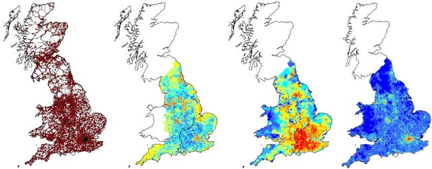
SSS10 Proceedings of the 10th International Space Syntax Symposium

Figure 1: UK’s A-roads model (left) and the GSE model (right).

There are representation issues to be dealt with, as the simplification and generalization of the
detailed geometries of non-relevant road features (as double-carriageways, roundabouts or highway
interchanges), which are non-trivial GIS processing tasks; on this subject see, for example, (Dhanani,
Vaughn et al. 2012). But both the Meridian 2 and the ITN are highly structured datasets, making such
tasks straightforward.

A number of common network centrality algorithms were run on these spatial models across a wide
range of radii, in order to test their adherence to reality, as described by four types of empirical data
(Figure 2): vehicular movement counts, the UK’s index of multi-deprivation (IMD), model-based
income estimates, and data on workplace zones’ population (a proxy of the location and density of
economic activities). All these datasets were provided by independent official sources (namely, UK’s
Office for National Statistics, ONS, and the Department for Transports, DfT).

Figure 2: Empirical datasets (from left to right): movement counts (5429 points), index of multi-deprivation
(31,672 LSOA polygons), model-based income estimates (7,194 MSOA polygons) and location of jobs (53,578
WZ polygons).

M Serra, B Hillier & K Karimi                                                                             84:4
Exploring countrywide spatial systems: Spatio-structural correlates at the regional and national scales
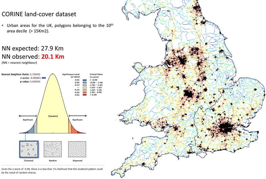
SSS10 Proceedings of the 10th International Space Syntax Symposium

The several datasets represented in Figure 2 have different territorial coverages and geographic
representations. Movement data 3 covers the entire country, and is represented as points located at
the geographic location of the measurement. Units are average annual daily flow (AADF) values, i.e.
the annual average number of vehicles passing daily at each observation point.

IMD data 4 covers the territory of England, and is encoded into Lower Super Output Area (LSOA)
polygons. These are relatively small areas of homogeneous population size (around 1,500 people),
but varying in area accordingly to spatial fluctuations of population density (therefore being much
smaller in cities than outside them). IMD units are abstract scores (calculated from 38 socio-
economic indicators), quantifying seven distinct domains of deprivation.

Income data 5 covers the territories of both England and Wales and comes in Medium Super Output
Area (MSOA) Polygons. MSOAs are larger than LSOAs, with a population of around 7,500 inhabitants;
MSOAs geometries are agglutinations of LSOAs (i.e. the latter are always perfectly contained in the
former). Income units are pounds sterling (values are model estimations), representing the average
net weekly income of the resident population.

Finally, working population data 6 (covering also England and Wales) is represented in Workplace
Zones (WZs) polygons: quite small areas (smaller than LSOAs) with approximately the same number
of workers (around 500), varying in area according to local densities of employing activities. As
LSOAs, WZs are significantly smaller in cities. The values are the number of people working at each
WZ, thus good proxies of employment and economic activities locations.

The processing of the several models used in this study was performed in depthmapX (Varoudis
2012), using three graph centrality algorithms constrained by metric radius, namely node count,
angular integration and angular choice. The historical space syntax terms of integration and choice
are equivalent to the more general terms of closeness and betweenness centralities (respectively),
used in the wider fields of mathematics, network physics and structural sociology. For generality
reasons, henceforth we will adopt the latter terminology, but when talking about closeness and
betweenness centralities, we will always be refereeing to the geometric-weighted versions of these
centrality algorithms, proposed by (Hillier and Iida 2005). Such algorithms, in particular
betweenness, are computationally demanding; current micro-computers can handle graphs with a
few hundreds of thousands of nodes, but processing time grows exponentially with graph-size. The
A-roads model used here, with 170,007 nodes, is well within the processing capabilities of micro-
computers, but the GSE model (1,342,365 nodes) and the full UK network model (2,031,971 nodes),
are at the very-limit of those capabilities. Their processing times, for a restricted number of radii
(maximum 100Km for GSE and 70Km for the complete model), was in the order of several weeks.
Therefore, one initial remark regarding the viability of the syntactic analysis of entire countries’
spatial networks, is the need to adopt parallel processing algorithms, common today in other
computing demanding fields but currently not implemented within space syntax software.

In Figure 3, we show the centrality patterns of angular closeness (radius 10Km) and angular
betweenness (radius 50Km), for both the A-roads and the GSE models. These two centrality
measures describe different things and thus produce quite different patterns. Closeness measures
the average angular distance of each node to all the others (or to those within radius), and
betweenness measures the number of times each nodes is part of the shortest angular paths
between all the other nodes (or between those within radius). Closeness, particularly at median radii
(e.g. 10 Km), typically produces patchy patterns of more central areas which, at the scale
represented in Figure 3, correspond to medium and large sized settlements. Betweenness typically
produces web-like patterns, corresponding to the most central paths of a spatial network. As we will
see, these specificities of closeness and betweenness are quite relevant to the crossing of spatial

3 Accessible at http://www.dft.gov.uk/traffic-counts/download.php
4 Accessible at http://data.gov.uk/dataset/index-of-multiple-deprivation
5 Accessible at http://www.ons.gov.uk/ons/rel/ness/small-area-model-based-income-estimates/index.html
6 Accessible at http://www.ons.gov.uk/ons/guide-method/geography/beginner-s-guide/census/workplace-

zones--wzs-/index.html

M Serra, B Hillier & K Karimi                                                                             84:5
Exploring countrywide spatial systems: Spatio-structural correlates at the regional and national scales
SSS10 Proceedings of the 10th International Space Syntax Symposium

centrality information with other types of data encoded in the three spatial data vector formats
(points, lines or polygons).

Figure 3: Centrality patterns of angular closeness at radius 10 Km (a and c) and angular betweenness at radius
50Km (b and d), for the A-roads and GSE models.

The processed network data was then imported into ArcGIS10 (ESRI 2011), as segment geometries
plus their centrality attributes, in order to be spatially related to the quantities described by all the
other previously mentioned empirical datasets. This was done by simple GIS analytical procedures,
spatially joining the attributes of the points or polygons with those of the segments they intersect,
who in turn hold a number of attributes describing their network centrality values across radii. In the
case of points (encoding vehicular movement data), the transfer of centrality attributes onto them is
direct, since the spatial relation is one of ‘one point / one segment’. In the case of data encoded into
polygons, which are intersected by a large number of segments, the centrality values of the
segments occurring within each polygon were averaged and then transferred to the corresponding
polygon. This method produced four data tables, whose lines correspond to spatial objects (points or
polygons), and columns correspond to attributes quantifying a given type of empirical phenomena
for that object (i.e. movement counts, socio-economic deprivation scores, income values and jobs
densities), and the average of the centrality values of the segments occurring within that spatial
object.

These data tables were afterwards studied through descriptive and correlational statistics, looking
for potential associations between spatial centrality variables and the variables describing the
functional and socio-economic phenomena mentioned before. Descriptive analysis included the
study of variables’ frequency distributions, transformations to normality and outlier analysis. In
general, numeric samples describing human geographic phenomena, as well as spatial network
centrality values, show long-tailed distributions of the log-normal type, which need to be
transformed to normality in order to meet the assumptions of parametric correlation methods. In
this work, we make extensive use of Pearson’s product-moment correlation coefficient as a measure
of the association between network centrality data and other socio-geographic data, and thus our
variables were in general log-transformed. The detection and isolation of extreme outliers (using the

M Serra, B Hillier & K Karimi                                                                             84:6
Exploring countrywide spatial systems: Spatio-structural correlates at the regional and national scales

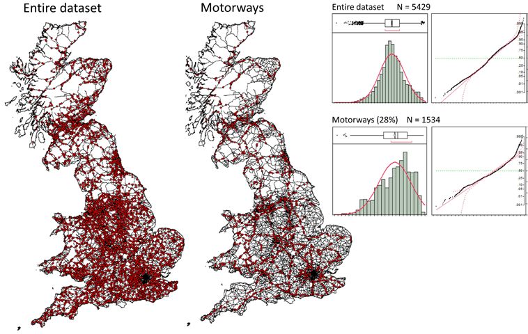
SSS10 Proceedings of the 10th International Space Syntax Symposium

inter-quartile range method 7) was performed in all variables, and such values were excluded from
correlation procedures.

Correlational analysis (using Pearson’s r) was systematically performed in search for significant
associations between network structure and the spatial distributions of movement and socio-
economic variables. Centrality variables were computed for a range of increasing radii, therefore
producing for each radius one correlation value with a given socio-economic variable. These values
may be plotted on line graphs, ordered from the lowest to the highest radius, making apparent the
trajectory of correlation values across spatial scales. In the following exercises, we will present our
results systematically in this way.

In order to evaluate the value of network structure as independent variable, we needed to compare
it with other independent environmental factors known to be associated with the type of socio-
economic phenomena addressed here. Of these, population density is perhaps the most recurrent,
known to be correlated with economic growth (Quigley 1998), crime incidence (Christens and Speer
2005), urban poverty (Tinsley and Bishop 2006) and innovation and employment opportunities
(Carlino, Chatterjee et al. 2007). In the following sections, whenever looking at correlations of
centrality values with socio-economic variables, we will always use the correlation with population
density as a benchmark value. We assume that, other things being equal, whenever correlations with
spatial measures are stronger (higher or lower) than with population density, we are in the presence
of a dependent variable that has a strong association with the structure of the spatial network.

3. Results
Postdicting vehicular movement at the national scale
The relation between the centrality hierarchy of human-made spatial networks and the distribution
of movement therein, is the key-stone of space syntax theory. We will, therefore, start by that
subject, using the sample of vehicular movement counts mentioned before. From the original
dataset provided by DfT, we selected a sub-sample of 5429 points occurring on A-roads, in order to
spatially relate those points with our model of the UK’s A-roads network (Figure 4).

Figure 4: Movement count samples, frequency distributions and Q-Q plots.

7This method defines an extreme outlier, as a value lying outside the interval [(Q1-3IQ), (Q3+3IQ)], where Q1
and Q3 are the first and third quartiles, respectively, and IQ is the inter-quartile range (Q3-Q1).

M Serra, B Hillier & K Karimi                                                                              84:7
Exploring countrywide spatial systems: Spatio-structural correlates at the regional and national scales
SSS10 Proceedings of the 10th International Space Syntax Symposium

This sub-sample is composed by count points on two main types of roads: principal and trunk roads,
PR and TR, and principal and trunk motorways, PM and TM. The distinction between trunk and non-
trunk roads is one of administrative nature (relative to the state agencies responsible for their
maintenance, the Secretary of State for trunk roads and Local Authorities for non-trunk roads). Their
distinction as motorways (PM, TM) and other A-roads (PR, TR) is more meaningful, for it corresponds
to actual physical differences of the infrastructure, namely quite different geometries and
connectivities. In order to investigate the performance of syntactic measures in postdicting
movement on these two different systems, we analyzed their correlations with the entire sample of
points (N=5429) and with just motorway points (N=1534). As Figure 4 shows, count points are rather
evenly distributed over the entire country, and the frequency distributions of logged movement
values are approximately normal.

The two movement samples were correlated with the centrality values of the segments intersected
by count points. Because the A-roads model is not too large (170,007 nodes) we were able to
process it for both closeness and betweenness along a wide range of radii, up to radius n. For each
centrality measure, the charts in Figure 5 plot the correlation values as two continuous curves (one
for the entire sample and another for motorways), making visible the evolution of the correlation
along spatial scales (all associated p-values are inferior to 0.001).

Figure 5: Correlations between centrality measures and movement data.

Starting from low r values at radius 1.2Km, the correlation curves rise very quickly, attaining
maximum and quite significant values at radius 20Km (10Km, for angular closeness with the entire
sample). The global maximum correlation is r=0.82, attained at radius 20Km for the motorway sub-
sample. Motorway traffic volumes are particularly well rendered (r=0.82 for closeness and r=0.63 for
betweenness), but correlations for the entire dataset are high as well (r=0.69 for closeness and
r=0.56 for betweenness). Given the size and the geographical coverage of the sample of count
points, these results leave little doubt that space syntax capacity for postdicting vehicular movement
flows remains entirely valid at very large territorial scales.

But the trajectories of the correlation curves also convey relevant information. In particular, the very
clear correlation peak around 20Km, preceded by a steep increase and followed by a softer (but no
less evident) decrease, consistent among measures and samples, seems to indicate a main scale for
M Serra, B Hillier & K Karimi                                                                             84:8
Exploring countrywide spatial systems: Spatio-structural correlates at the regional and national scales
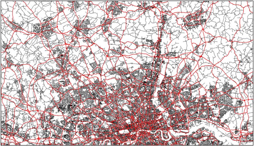
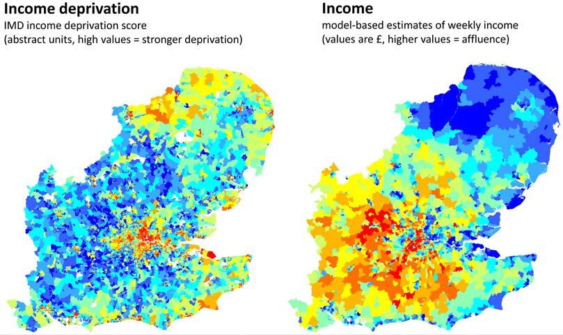
SSS10 Proceedings of the 10th International Space Syntax Symposium

movement at the national level; while also suggesting that the centrality hierarchy of the network
itself, must somehow embody this particular territorial scale.

And, indeed, some additional elements regarding patterns of travel behavior and of territorial
occupation in the UK, support the likelihood of these results. In 2013, the global average trip length
in England was 11.43 Km, the average commuting distance was 14.16 Km and the average day trip
was 21.24 Km (DfT 2013); all these values oscillate around the scale at which highest correlations are
attained in our analysis.

Figure 6: Average nearest neighbour distance between main settlements in Britain.

The CORINE land-cover dataset (EEA 2009) was used to study UK’s generic geographical distribution
of urban areas. We isolated the CORINE polygons classified as urban and belonging to the 10th area
decile (>15 Km2) of the total distribution of urban polygons’ areas. This produced a sample of 349
polygonal shapes, with areas ranging from 15 Km2 to 3065 Km2 (mean 75 Km2, standard deviation
208 Km2), representing the general spatial distribution of settlements in the UK (Figure 6). We then
applied on this sample a common geo-statistical calculation in GIS – average nearest neighbor (ANN)
estimation – to produce a value capable of describing the average distance between urban areas in
the UK, obtaining a result of 20.1 Km. Even if a rough estimation, this value also strongly supports
the validity of the abovementioned findings.

Describing poverty and affluence at the regional scale
Once assured a basic condition for extending space syntax analysis to the regional and national
territorial scopes – namely the validity of the relationship configuration / movement – we now look
at possible associations with the spatial distributions of socio-economic variables. The high
granularity with which this type of data is provided, led us to use a detailed model for this exercise,
namely the GSE model.

Two types of socio-economic variables were initially accessed. Income deprivation, one of the
domains of the IMD, quantified as an abstract score and encoded into LSOA polygons; and average
household income per week, computed by model-based estimates (combining survey, census and
administrative data), quantified in Pounds Sterling and encoded in MSOA polygons. The former

M Serra, B Hillier & K Karimi                                                                             84:9
Exploring countrywide spatial systems: Spatio-structural correlates at the regional and national scales
SSS10 Proceedings of the 10th International Space Syntax Symposium

variable measures the proportion of the population in a LSOA experiencing deprivation related to
low income (i.e. people claiming benefits or other allowances), with higher values revealing a highly
impoverished area. The latter variable, measures the average net week income of the households
occurring in each MSOA, with higher values indicating a highly affluent area. It is important to stress
that both variables are not complementary or mutually exclusive. Income deprivation quantifies only
the number of deprived people as a proportion of the total – it does not imply in any way the total
absence of affluent inhabitants. Likewise, an area with a high average household income, does not
imply the inexistence of poor households in that area, but only that the average is high (Figure 7).

Figure 7: Datasets of income deprivation and medium weekly income.

A quick visual inspection of the patterns depicted in Figure 7 is enough to suggest some obvious
differences between the main geographic trends of poverty and affluence in the area covered by the
GSE model. Poverty (i.e. income deprivation) concentrates in urban areas but also in remote areas,
as the coasts of Norfolk and Suffolk. The countryside and the areas in-between cities show much
lower income deprivation values. Affluent areas, on the contrary, tend to occur not so much at cities,
but rather on the areas surrounding them and in particular to the west and south of London. Two
opposed generic patterns, suggesting clear spatial cleavages and different location behaviours of
impoverished and affluent populations.

We explored the relations between the spatial distributions of these two socio-economic variables
and the structure of the spatial network, by averaging the angular closeness values of the segments
intersecting each polygon, and then correlating that value with those of the two variables. This was
done along several radii, from the very local scale (800m) to the large regional scale (100Km). For the
reasons stated before, we check also the correlation of population density with income deprivation
and average income, and set those two values as benchmarks to access the relative importance of
spatial centrality as independent variable.

As mentioned before, certain differences between the centrality structures that closeness and
betweenness describe, have a bearing on their potential association with other data in GIS. Indeed,
in the case of data described by areal objects (i.e. regions or polygons), the patchy centrality
structures brought to light by closeness are much easier to associate with areal data than the web-
like structures revealed by betweenness. This is also in part a consequence of the method of spatial
averaging used here, because locally, closeness centrality values vary less than betweenness values,
and thus their local averaging correctly describes them. At any rate, in the exercises carried out in

M Serra, B Hillier & K Karimi                                                                             84:10
Exploring countrywide spatial systems: Spatio-structural correlates at the regional and national scales
SSS10 Proceedings of the 10th International Space Syntax Symposium

this work, closeness has always produced stronger associations with data described by areal objects;
in the following sections, our results will always refer to correlations with closeness centrality.

Figure 8: Correlations between angular closeness and income deprivation (red curve) and income (blue curve).
The respective correlations with population density are represented by dashed lines.

The results, reported on Figure 8, show that both income deprivation and average income attain
significant positive correlations with spatial centrality values (r=0.40 and r=0.47, respectively). The
maximum correlations with angular closeness are superior to the correlations with population
density (overwhelming so, in the case of income), showing that spatial structure is indeed a better
descriptor of these two socio-economic variables. The trajectories of the correlations across radii are
also very different for each variable. The curve describing the correlation with income deprivation is
positive (r=2.7) at low radii (0.8 Km), attains it maximum at 2.4 Km (r=0.4) and then decreases
symmetrically, reaching a value close to r=0 at 100 Km. The curve describing average income follows
an almost opposed trajectory, starting negative (r=-0.1) at 0.8 Km, and then increasing continuously
until its maximum (r=0.47) at 100 Km.

These results show that income deprived population concentrates in areas with high accessibility at
the city-scale, in fact the actual city centres. Whereas affluent population concentrates in areas with
high accessibility at the region-scale, which clearly outstrip urban limits (see centrality patterns of
Figure 8). Again, this does not mean the absence of affluent people in cities, or the absence of
poverty outside them. That could only be said if strongly negative correlations were also to be
observed for both variables, at the city scale for affluence and at the regional scale for income
deprivation. But what these results do mean, is that affluence is non-characteristic in cities and
poverty is in non-characteristic in rural areas (i.e. that they are not representative in each case). And
what the results also show, is that the structure of the spatial network has a clear bearing on this
socio-spatial cleavage, or that at least is capable of better describing it than simple population
density (Figure 8).

Exploring the association between multi-deprivation domains and spatial accessibility: the
fundamental role of the background network
These encouraging signals of potential associations between spatial accessibility and the territorial
distribution of socio-economic phenomena at the regional scale, were further investigated through

M Serra, B Hillier & K Karimi                                                                             84:11
Exploring countrywide spatial systems: Spatio-structural correlates at the regional and national scales
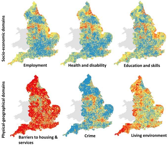
SSS10 Proceedings of the 10th International Space Syntax Symposium

the several domains of the UK’s Index of Multiple Deprivation. But in this exercise we also
investigate another issue. Because we have two models representing different partitions of UK’s
spatial network – one covering the entire country, but including only A-roads; and another, covering
the GSE area but including every street – we may study comparatively their results, in order to
understand the relations and relative importance of the background and foreground networks, as
described and theorized by Hillier (2012) (Figure 9); and also to ascertain the degree of relevance
that the background network may have in making very large syntactic models more or less predictive
(i.e. if the background network is indeed indispensable in modelling terms).

Figure 9: The A-roads model (red) superimposed over the GSE model (black): the foreground and the
background networks.

A brief review of the several IMD domains and of the deprivation aspects each one quantifies, is
necessary to make the following results clear. The English Indices of Deprivation use 38 separate
indicators, which are combined, using appropriate weights, to calculate seven main domains of
deprivation (DCLG 2011). Apart from income deprivation, a domain that was already explored in the
previous section, the six remaining IMD domains are: employment deprivation, health deprivation
and disability, education and skills deprivation, barriers to housing and services, crime and quality of
living environment (Figure 10, next page).

Employment deprivation describes the proportion of working age people living in an area, which are
involuntary excluded from the labour market (i.e. the proportion of unemployed, but job seeking
people). Health deprivation and disability, measures premature death and the impairment of quality
of life by poor health (described by morbidity, physical and mental disability and premature
mortality). Education and skills deprivation, measures the extent of lack of formal education and
professional skills. Barriers to Housing and Services, measures the physical and financial accessibility
of housing and key local services. Crime, measures the rate of recorded crime (violence, burglary,
theft, criminal damage), representing the risk of personal and material victimization on a given area.
Quality of Living Environment, measures the quality of individuals’ immediate surroundings both
within the home (poor conditions of social and private housing, and the lack of central heating) and
outside it (air quality of the area and the proportion of road traffic accidents), (DCLG 2011). In order
to make our results clearer, we organised these six domains into two groups: one composed by
domains not obviously spatially or environmentally related (employment, health and disability,
education and skills) – which we term socio-economic domains – and another composed by domains
which potentially depend on spatial and environmental conditions (barriers to housing and services,
crime and quality of living environment) – which we term physical-geographical domains (Figure 10).

M Serra, B Hillier & K Karimi                                                                             84:12
Exploring countrywide spatial systems: Spatio-structural correlates at the regional and national scales
SSS10 Proceedings of the 10th International Space Syntax Symposium

Figure 10: The several domains of the Index of Multi-Deprivation.

Perhaps the most staggering aspect of IMD spatial distributions depicted in Figure 10, is the
concentration of highly deprived areas in cities (DCLG 2011). Except for ‘barriers to housing and
services’ (which are higher in rural areas), and to a certain extent also ‘quality of living environment’
(which, albeit high in cities, it is also high on remote areas), all the other domains attain their
maximum scores in urban areas. One could almost say that social deprivation follows an urban/rural
pattern of spatial distribution. It is thus expected that all IMD domains will be significantly correlated
with population density. So we will again use population density as a benchmark variable to assess
the discriminant value of space syntax spatial centrality measures. Whenever correlations with those
variables are higher than with population density (in absolute value), we may assume a strong
association with the structure of the spatial network. The method for aggregating IMD scores and
spatial accessibility values is similar to the one described before, but now we use two spatial
networks. Again, we average the centrality values of the segments of each network occurring in each
polygon, and then compare those averages with IMD scores. We thus obtain two correlation curves
for each IMD domain (see Figure 11).

Employment deprivation and health deprivation and disability are more associated with population
density than with spatial structure, even if the correlation difference between them is quite small.
Education and skills deprivation show a suggestive (albeit weak) negative correlation (r=-0.24) at 100
Km which, we recall, was also the spatial scale at which the maximum correlation with economic
affluence was attained (see Figure 8); the well-known relationship between economic affluence and
education levels (Filmer and Pritchett 1999) seems to be captured here, and more effectively
through centrality measures. The physical-geographical domains, i.e. those more related to spatial
factors (barriers to housing and services, crime and living environment) are definitively more
associated with spatial structure than with population density, attaining significantly higher absolute
correlation values with centrality measures. Moreover, the results tell us at which spatial scale such
associations are maximized (i.e. the radius of analysis at which the maximum correlation is attained).
Barriers to housing and services show a strong negative correlation (r=-0.67) at radius 2 Km,
reflecting the fact that this type of deprivation is much less common in cities, and in particular at
their centres (which have high centrality values at that spatial scale). Crime and living environment

M Serra, B Hillier & K Karimi                                                                             84:13
Exploring countrywide spatial systems: Spatio-structural correlates at the regional and national scales
SSS10 Proceedings of the 10th International Space Syntax Symposium

attain maximum correlations (r=0.66 and r=0.74, respectively) at radius 10 Km, which is roughly the
spatial scale at which main urban areas are highlighted (see centrality patterns of Figure 3).

Figure 11: Correlations between IMD domains and spatial accessibility (closeness), for A-roads (blue curves) and
for the complete GSE network (red curves). The horizontal lines represent the correlations between domains
scores and population density.

But the charts in Figure 11 point also to two other important facts. The first is that, in spite of the
very different sizes of the two models used in this exercise, the results are surprisingly convergent
beyond a certain spatial scale (circa 5 or 10 Km; we do not have data for the GSE model above 100
Km radius, due to lack of processing capability). This shows, on one hand, the high robustness and
stability of space syntax measures and models and, on the other hand, that beyond that scale the
foreground network is the main factor of association and the background network becomes
irrelevant. But the results also tell us a second and very important fact: that below that same scale (5
– 10 Km), the background network (present in the GSE model) assumes a very relevant role, while
the foreground network is incapable of capturing associations with the studied variables (Figure 12).
In other words, phenomena related to the micro-structure of spatial networks (as barriers to housing
and services, in this case) may only be captured with models including both background and
foreground networks. This clearly highlights the need for complete, nationwide spatial network
models.

M Serra, B Hillier & K Karimi                                                                             84:14
Exploring countrywide spatial systems: Spatio-structural correlates at the regional and national scales
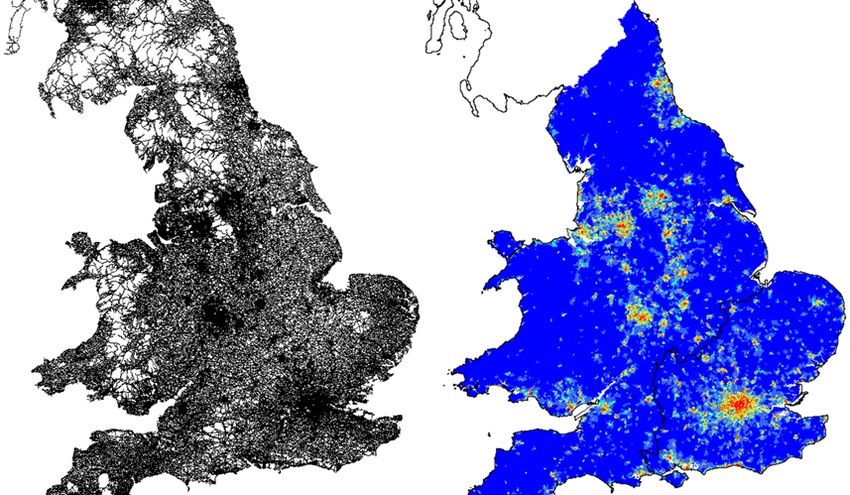
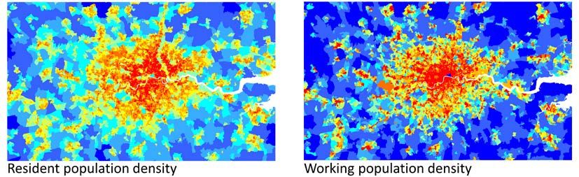
SSS10 Proceedings of the 10th International Space Syntax Symposium

Figure 12: Concordance and divergence between the A-roads and the GSE models.

Spatial micro-structure and the location of economic activities
We need complete models if we are to observe phenomena at the micro-scale (i.e. at the
neighborhood and inner city scales). In other words, we need to compute each and every street of
entire countries, a task that is at the very limit of current micro-computers’ processing capabilities.
Notwithstanding, we produced one model of the entire UK road network (Figure 13) on which work
is still on-going; we report here some preliminary findings in order to illustrate the relevance of
spatial micro-structure in very large syntactic models. For this exercise we used yet another type of
empirical data, namely values of working population per workplace zone 8 (WZ), which is a direct
indicator of the location of jobs and economic activities. The dataset used for this, provided by ONS,
pertains to the entire territories of England and Wales, and is composed by 52,896 WZ polygons
(Figure 13).

Figure 13 shows that the highest densities of jobs, and thus of economic activities, occur
overwhelmingly in cities; a fact only to be expected. However, such fact also means that, once again,
population density is bounded to be highly correlated with job density. And indeed it is, yielding
r=0.62. For that reason, we use population density in this exercise again as a benchmark variable,
against which one may access the bearing that network structure may have on the distribution of
economic activities.

The spatial distributions of resident and working populations, although fairly similar, show some
important differences (Figure 14). Working population density has a highly heterogeneous spatial
distribution, with high densities clustered in specific areas, surrounded by a general background of

8WZs were introduced in the 2011 census and are designed to supplement the output area (OA) and super
output area (LSOA and MSOA) geographies. OAs were originally created for the analysis of population statistics
using residential population and household data, but they are of limited use for workplace statistics. OAs are
designed to contain consistent numbers of persons, based on where they live, WZs are designed to contain
consistent numbers of workers, based on where people work.

M Serra, B Hillier & K Karimi                                                                             84:15
Exploring countrywide spatial systems: Spatio-structural correlates at the regional and national scales
SSS10 Proceedings of the 10th International Space Syntax Symposium

less denser areas; whereas population density shows a more even pattern, without such marked
variations. The hypothesis put forward here, is that these differences may be explained by also
marked variations in network structure and spatial accessibility.

Indeed, as Figure 15 shows, both angular closeness and node count, attain much higher correlations
than population density, at radii 2Km and 10Km. Node count at 2Km is actually capable of explaining
66% of the variance of working population density (see inset scattergram, Figure 14).

Figure 13: The complete UK’s spatial network model and the working population dataset.

Figure 14: Spatial distributions (London area) of resident and working population densities.

However, beyond those scales, correlations drop quickly, namely below the benchmark line of
population density. As shown in the previous section, the scales below 10Km are those at which the
background network becomes highly relevant. Therefore, a country-sized model of the UK, but
representing only the foreground network, would completely fail to detect such an important
functional association with spatial structure, one that could have direct implications to the
understanding of the economic performance of cities. Such a powerful, concise an locally precise
description of a phenomenon as complex as job location at the scale of an entire country, may
therefore only be attained through national sized, but no less exhaustive, spatial network models.

M Serra, B Hillier & K Karimi                                                                             84:16
Exploring countrywide spatial systems: Spatio-structural correlates at the regional and national scales
SSS10 Proceedings of the 10th International Space Syntax Symposium

Figure 15: Correlations between spatial measures and working population density.

4. Conclusions
In this paper we reported the results of a series of exercises carried out in order to access the validity
of space syntax analysis at very-large spatial scales, namely that of entire countries. Today, the
widespread availability of GIS road-centre line data has made the creation of country-wide syntactic
models possible, but their processing times with current micro-computers and standard network
analysis software are still extremely long. In order to make the syntactic analysis of entire countries
fully operational, massive parallel processing technologies should be adopted, as they have been in
other fields of research demanding data-intensive computing.

Notwithstanding these limitations, we have provided evidence that such path may be broke. Using
the UK spatial network as case study, we shown that both at the regional, supra-regional and even
national scales, syntactic models and analysis hold all their relevance, showing clear associations
with functional and socio-economic phenomena, as described by datasets covering the entire UK’s
mainland territory.

The fundamental idea underpinning space syntax theory – the relationship between spatial
configuration and movement rates – was shown to be entirely valid at the country-wide scales.
Movement flows are effectively described by space syntax topo-geometric centrality measures and
regional movement seems to be particularly well rendered. Socio-economic variables, describing
social deprivation, economic affluence and employment location are also well captured at very-large
spatial scales, showing strong statistical associations with spatial structure which are consistent with
known sociological and demographic trends, while adding to that knowledge the spatial accuracy
that syntactic analysis provides.

The correlations found are not only significant, but they are also very consistent between datasets of
different origins and dimensionality, both geographical and thematic. Therefore we may conclude
that syntactic analysis at country-wide territorial scales is not only valid, but highly relevant and a
promisingly fertile subject of research.

M Serra, B Hillier & K Karimi                                                                             84:17
Exploring countrywide spatial systems: Spatio-structural correlates at the regional and national scales
SSS10 Proceedings of the 10th International Space Syntax Symposium

References
Batty, M. (2005). Cities and Complexity: Understanding cities through cellular automata, agent-based models
         and fractals. Cambridge, MA, MIT Press.
Batty, M. (2008). ‘The Size, Scale and Shape of Cities.’ Science 319, p.769-771.
Carlino, G., S. Chatterjee and R. M. Hunt (2007). ‘Urban density and the rate of invention.’ Journal of Urban
         Economics 61, p.389-419.
Christens, B. and P. W. Speer (2005). ‘Predicting Violent Crime Using Urban and Suburban Densities.’ Behavior
         and Social Issues 14, p.113-127.
DCLG (2011). The English Indices of Deprivation 2010, Department for Comunities and Local Governement - UK
         Government.
DfT (2013). Annual Road Traffic Estimates: Great Britain 2013, Department for Transport - UK Governement.
Dhanani, A., L. Vaughn, C. Ellul and S. Griffiths (2012). From the Axial Line to the Walked Line: evaluating the
         utility of commercial and user‐generated street network datasets in space syntax analysis. Eighth
         International Space Syntax Symposium, Santiago de Chile, PUC.
EEA (2009). CLC2009 Technical Guidelines. Copenhagen, EEA, European Environment Agency
ESRI (2011). ArcGIS Desktop: Release 10. Redlands, CA, Environmental Systems Research Institute.
Filmer, D. and L. Pritchett (1999). ‘The Effect of Household Wealth on Educational Attainment: Evidence from 35
         Countries.’ Population and Development Review Vol. 25(1), p.85-120.
Hillier, B. (1999a). Space is the Machine: A Configurational Theory of Architecture. Cambridge, Cambridge
         University Press.
Hillier, B. (1999b). ‘The Hidden Geometry of Deformed Grids: or, why space syntax works, when it looks as it
         though it shouldn’t.’ Environment and Planning B: Planning and Design Vol. 26(2), p.169-191.
Hillier, B.; Iida, S. (2005). ‘Network and psychological effects in urban movement.’ In: Cohn, A.G. and Mark,
         D.M., (eds.) Proceedings of Spatial Information Theory: International Conference, COSIT 2005,
         Ellicottsville, N.Y., U.S.A.,September 14-18, 2005 (475-490). Springer-Verlag: Berlin, Germany.
Hillier, B. (2012). ‘The genetic code for cities: is it simpler than we thought ?’ Complexity Theories of Cities have
         come of age: an overview with implications to urban planning and design. M. H. Portugali Y., Stolk E. and
         Tan E. (eds.), Springer Complexity.
Kalapala, V., Sanwalani, V., Clauset, A., Moore, C. ‘Scale Invariance in Road Networks.’ Physical Review E 73, p.
         026130.
Quigley, J. (1998). ‘Urban Diversity and Economic Growth.’ The Journal of Economic Perspectives Vol. 11(2),
         p.127-138.
Reis, A. H. (2007). ‘Constructal view of the scalling laws of street networks – the dynamics behind geometry.’
         Physica A 387, p.617-622.
Tinsley, K. and M. Bishop (2006). ‘Poverty and Population Density: Implications for Economic Development
         Policy.’ Journal of Higher Education Outreach and Engagement Vol. 11(1), p.195-207.
Turner, A. (2007). ‘From axial to road-centre lines: a new representation for space syntax and a new model of
         route choice for transport network analysis.’ Environment & Planning B: Planning and Design Vol. 34(3),
         p.539-555.
Varoudis, T. (2012). depthmapX Multi-Platform Spatial Network Analysis Software.
Zhang, H., Li, Z. (2011). ‘Fractality and Self-Similarity in the Structure of Road Networks.’ Annals of the
         Association of American Geographers Vol. 102(2), p.350-365.

M Serra, B Hillier & K Karimi                                                                                  84:18
Exploring countrywide spatial systems: Spatio-structural correlates at the regional and national scales
You can also read