GRAPH NEURAL NETWORKS TO PREDICT CUSTOMER SATISFACTION FOLLOWING INTERACTIONS WITH A CORPORATE CALL CENTER
←
→
Page content transcription
If your browser does not render page correctly, please read the page content below
G RAPH N EURAL N ETWORKS TO P REDICT C USTOMER
                                                   S ATISFACTION F OLLOWING I NTERACTIONS WITH A
                                                              C ORPORATE C ALL C ENTER

                                                                                               A P REPRINT

                                                      Teja Kanchinadam, 1 Zihang Meng, 2 Joseph Bockhorst, 1 Vikas Singh, 2 Glenn Fung 1
arXiv:2102.00420v1 [cs.LG] 31 Jan 2021

                                                                 1
                                                                   American Family Insurance, Machine Learning Research Group
                                                                               2
                                                                                 University of Wisconsin - Madison
                                                             {tkanchin, jbockhor, gfung}@amfam.com, {vsingh, zmeng29}@wisc.edu

                                                                                             February 9, 2021

                                                                                              A BSTRACT
                                                  Customer satisfaction is an important factor in creating and maintaining long-term relationships with
                                                  customers. Near real-time identification of potentially dissatisfied customers following phone calls
                                                  can provide organizations the opportunity to take meaningful interventions and to foster ongoing
                                                  customer satisfaction and loyalty. This work describes a fully operational system we have developed
                                                  at a large US company for predicting customer satisfaction following incoming phone calls. The
                                                  system takes as an input speech-to-text transcriptions of calls and predicts call satisfaction reported
                                                  by customers on post-call surveys (scale from 1 to 10). Because of its ordinal, subjective, and often
                                                  highly-skewed nature, predicting survey scores is not a trivial task and presents several modeling
                                                  challenges. We introduce a graph neural network (GNN) approach that takes into account the
                                                  comparative nature of the problem by considering the relative scores among batches, instead of
                                                  only pairs of calls when training. This approach produces more accurate predictions than previous
                                                  approaches including standard regression and classification models that directly fit the survey scores
                                                  with call data. Our proposed approach can be easily generalized to other customer satisfaction
                                                  prediction problems.

                                         1   Introduction
                                         Improving customer loyalty and tenure are crucial components of business success. As there is an industry-wide
                                         consensus that customer satisfaction is significantly correlated to customer attrition [1], understanding and improving
                                         customer satisfaction are core elements of the strategy of many organizations.
                                         One aspect of understanding overall customer satisfaction is to monitor and study its determinants within individual
                                         interactions, such as phone calls, that customers have with the organization. Indeed many businesses conduct automated
                                         and / or live customer satisfaction surveys following interactions with corporate call centers. However, due to extremely
                                         low response rates, especially for automated surveys, along with the high costs of live surveys, typically only a small
                                         percentage of calls have satisfaction scores. Moreover, live calls often have a significant time lag (a week or more)
                                         making it difficult to quickly monitor, recognize and respond to both trends and individual cases. In this paper we
                                         investigate an approach for shedding light on these unobserved interactions using speech-to-text models and supervised
                                         learning.
                                         In previous work we have found that predictions of customer satisfactions derived from simple linear pairwise-ranking
                                         models to be a better fit than standard regression methods [2], likely due to the ordinal scale of the target variable (the
                                         survey responses). We hypothesize, however, that as the relationship between call text and satisfaction is complex and
                                         likely non-linear, appropriate non-linear models will lead to more accurate predictions. Here we adapt an approach
                                         based on graph neural networks (GNN) [3] that has previously been found to be effective for non-linear ranking
                                         problems.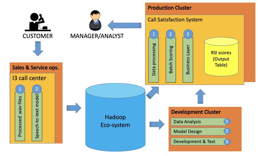
A PREPRINT - F EBRUARY 9, 2021

Figure 1: Example - if we are learning to rank cats by age, looking at groups of cats ordered by age simultaneously will
provide a more compact representation of the information to the learner than having to learn by only looking at a pair of
cats at one time.

                                      Figure 2: Overview of the deployed system

An advantage of the GNN formulation over non-linear pairwise ranking models is that under the GNN predicted
rankings for a batch of examples is guaranteed to be coherent with respect to the transitive nature of a ranking. A
non-linear pairwise model, on the other hand, has no structural constraint preventing an incoherent set of predictions
such as a > b, b > c and c > a. Additionally, the GNN may consider higher order features (ie, non-pairwise) among
the examples. For example, if we are learning to rank cats by age (Figure 1), looking at groups of cats ordered by age
simultaneously will provide a more compact representation of the information to the learner than learning by only
looking at one pair of cats at time. Indeed, our experimental results (Section 4) indicate that GNN models provide the
most accurate predictions among a set of alternative approaches.
The rest of the paper is as follows. First we provide an overview of the deployed system (Section 2) and describe the
details GNN model (Section 3). Next we describe our experimental methods and results (Section 4), the system as
deployed (Section 5), and related work (Section 6). Last, we discuss future work and our conclusions (Section 7).

                                                           2
A PREPRINT - F EBRUARY 9, 2021

2   System Overview

Our company uses a third party speech-to-text software to transcribe the incoming call center calls. The files of the calls
are converted into text-based-files that contain the transcription of words produced during the conversation between the
caller (customer) and the customer representative. The transcription also automatically detects and maps utterances to
speakers and all this extra information is provided with the transcriptions.
The company customer care center monitors customer satisfaction by offering surveys conducted by a third party vendor
to 10% of incoming calls. Due to low response rates, however, fewer than 1% of all incoming calls have completed
surveys. This corresponds to an average of approximately five surveys completed per month per representative. There
are four topics measured by the survey: (a) If the customer felt “valued” during the call; (b) If the issue was resolved;
(c) How polite the CR was, and (d) How clearly the CR communicated during the call. Scores range form 1 to 10 (1
lowest, 10 highest) and the four scores are averaged into an additional variable called RSI (Representative Satisfaction
Index). In this paper we focus on predicting the RSI.
More formally, the final modeling task is to learn a function f (x) = ŷ, mapping any given feature vector x to a predicted
RSI ŷ such that on an average the difference between the predicted score and actual score y is small.
Several challenges, in terms of modeling, are discovered after a quick initial inspection of the available training data:

       • The RSI scores are highly biased towards the highest score (10), while calls with scores lower than 8 are less
         than 4%. This highly skewed distribution makes building a predictive model challenging.
       • Survey scores are customer responses, thus are subjective, qualitative states heavily impacted by personal
         preferences.
       • The measurement scale of survey scores is ordinal; one cannot say, for example, that a score of 10 indicates
         double satisfaction as a score of 5. Most, if not all, standard regression techniques implicitly assume an interval
         or ratio scale.

Even when the final objective of the system is to predict the actual RSI scores, because of the reasons mentioned above,
we propose a two-phase strategy: First we learn a model to learn a relative ranking score for the calls (ordinal ranking)
and then we map the ranking score to satisfaction scores in the 1-10 scale.
The system workflow is illustrated in Figure 2 and it can be summarized by the following steps:

      1. After a call ends, a transcript of the call is automatically produced by a speech-to-text software developed by
         Voci (vocitec.com).
      2. Features are calculated for each call transcript using a word embedding model trained on more than 2 million
         documents including transcribed calls (for which we don’t have survey scores) and other insurance-related text
         corpus available within the company. The resulting feature vectors are used as input features for the models
         described in the next step.
      3. Ranking model: The ranking model is trained by sampling batch of calls and feeded into the GNN framework.
         The ranking loss is calculated based on the corresponding satisfaction scores.
      4. Mapping from raking scores to satisfaction scores is performed using an Isotonic Regression (IR) model [4]
         and thus individual (per call) satisfaction predictions are generated.
      5. Aggregation of calls at the group level are stored in a database. Example groups include: per CR, per queue
         and per time period.
      6. Aggregations are used for real-time reporting though a monitoring dashboard.

3   Learning rankings using GNNs

Inspired by the approach proposed in [3], our approach is based on the fact that when ranking customer calls by
satisfaction level, the learning algorithm can benefit from having access and hence exploring the similarity among
multiple calls (instead of only considering pairs of calls) represented on a graph, where each node represents a call and
the edges are learned based on the relationship between the to-be-learned representations of the nodes.
Each phone call transcript is represented by an embedding vector (as described in detail in a later section) and are
mapped into the graph representation. Details of our network architecture for rank learning are presented next.

                                                             3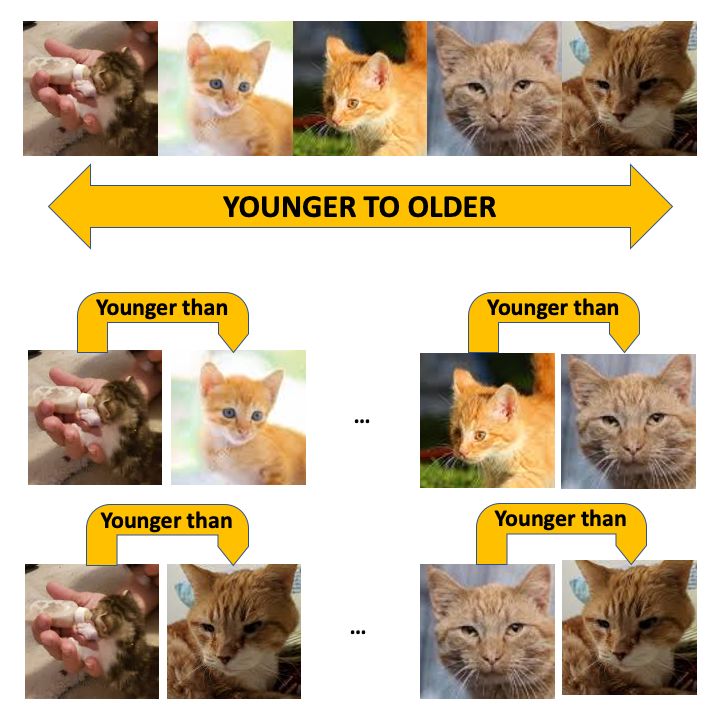
A PREPRINT - F EBRUARY 9, 2021

Figure 3: Overview of the framework. The weights in the entire framework including those in the CNN and GNN
are trained end-to-end. The edges on the graph are learned from adjacent nodes using a parametrized function (ϕϑ ,
equation. (2)), which is shared among all edges. The messages are passed to every node from its connected nodes and
edges as defined in equation. (3). A GRU cell combines node information and its corresponding messages generating
the output. The parameters in GRU are also shared across all the nodes.

3.1   Network Architecture

Let C = {C1 , C2 , · · · , Cn } be the set of input calls, we assume that a set of pairwise relationship labels PLt =
{L(Ci , Cj )}ni,j=1;i6=j , where L(Ci , Cj ) indicates the relative goodness (based on survey scores) between the two calls
Ci and Cj . Given this data, a generalized GNN is trained where both the node features (embedding representations of
the call transcripts) and edge weights are learned. The core architecture of our GNN is shown in Fig. 3.
As described in [3], we will assume that we operate on groups (or mini-batches) of a certain size (which are allowed
to vary) sampled with or without replacement from the underlying training dataset. The relationships among all the
calls in each mini-batch (S) in the training set are represented using a fully-connected graph GS = (V, E), where each
node vi in V corresponds to a call Ci in the mini-batch S. For each batch S, the network takes in a group of calls and
calculates the corresponding initial vectorial embedding representation xi = f (Ci ) ∈ IRn , where f (·) refers to a text
embedding function. Note that in [3], the architecture presented considers several layers of connected Gated Recurrent
Units (GRU) in a sequential manner. For this work we only consider one layer since in practice several layers did not
improve model accuracy significantly, at least for our problem. Next, the network learns edge features as,

                                                   ei,j = ϕϑ (xi , xj ) ,                                              (1)

where ϕ is a symmetric function parameterized with a single layer neural network:

                            ϕϑ (xi , xj ) = ReLU W |x1i − x1j |, . . . , |xni − xnj | + b .

                                                                                                                       (2)

Here xji denotes the j th component of the embedding vector xi . In other words, ϕ is a non-linear combination of the
absolute difference between the features of two nodes, W and b are the weight matrix and the bias respectively, and
ReLU(·) is the rectified linear unit (ReLU) function.
To update the information considered at each node based on the information at the other nodes in the graph, we use
a message function M (·) to aggregate evidence from all neighbors of each node. For each node xi , the message is
defined as below,
                                                   X
                                             mi =      M (xj , ei,j ) .                                        (3)
                                                       j,j6=i

                                                                4
A PREPRINT - F EBRUARY 9, 2021
Where M (·) is parameterized using a single layer neural network and is defined as below,
M (xj , ei,j ) = ReLU (W (xj kei,j ) + b) , (4)
Here k denotes the concatenation operator of two vectors, The parameters (W and b) of the message function M (·) are
shared by all nodes and edges in our graph, thus providing an explicit control on the number of parameters and making
the architecture more modular, allowing us to train and perform inference with different configuration of networks
according to the problem needs.
The edge features are learned as suggested by Gilmer et al. [5] and described in equation (1). The parameters of
the edge learning function ϕϑ are also shared among all nodes on the graph. Then for every node xi in the graph, a
"summarized" message signal will be extracted from all the inputs and edges of this node, see (3). For each node, we
use a GRU that combines the messages received from the node’s neighbors and its corresponding input x0i to produce
an output through a readout function oi = R(xi , mi ).
It is important to note that GRU units are known for their use in sequence problems. However, we are using them for a
different purpose in this work. The purpose of the GRU units in this architecture is to capture and learn simultaneously
the relative relations among examples in a given batch.
For our specific task of ranking calls, we use a classic ranking loss as described in [6]. This formulation is robust to
noise and is symmetric by construction so it can easily utilize batches of training data where some pairs of calls have
“equal” scores, which is often the case here since our scores distribution is highly skewed towards 10. See Fig. 4. Hence,
the loss function for any pair of calls Ci and Cj defined on the output of the graph takes the form
X
RALLoss = −L log(Pij ) − (1 − L) log(1 − Pij ), (5)
i,j,i6=j
where
1 if Si Sj ,
L= 0 if Si ≺ Sj ,
0.5 otherwise,
and Pi,j = oi − oj (outputs of nodes i and j). Where Si is the corresponding satisfaction score for call Ci .
This loss seeks to learn a network that, given the input calls, it simultaneously outputs pairwise labels according to the
relative strength of certain attributes between each pair of calls. In this paper, we consider training a network for one
attribute (RSI) at a time. However this framework can be also use to learn several tasks at the time (multi-task learning)
as described in [3].
Our network is designed to better explore the correlated information among a batch or a group of different calls. So
unlike other approaches related to relative attribute learning (including Siamese-network-based) [7, 8, 2] which typically
take only two training examples at a time as an input, we sample a potentially arbitrary size group of calls from the
training set as input at every draw. The size of the group need not be fixed and can be variable for learning different
attributes in a single dataset or different datasets, since our network has the benefit of weight sharing on the graphical
structure of the samples.
For some of our experiments, we have used the architecture of CNN described in [9] with the same number of filters and
static representation of the word vectors. For the initialization of the words we have used the word vectors described in
Section 4.2. The dimension of the output feature vector will be the sum of individual filter sizes multiplied by their
respective feature maps.
As proposed in [3], we also impose a fully-connected graphical structure on the calls in each group.
Each GRU takes the input representation for a node and it’s incoming message summary as an input, and produces the
output (see Fig. 3). Let x0i be the node’s input representation (obtain by the CNN layer), mi be the message received via
(3), and oi be the output of node through the readout function. With these notations, for our case, the basic operations
of GRU are simply given as,
zi = σ W z mi + U z x0i , rv = σ W r mi + U r x0i and
õi = tanh W mi + U ri x0i , (6)
oi = (1 − zi ) x0i + zi õi
where z and r are the intermediate variables in the GRU cells (update and reset gates), σ(x) = 1/(1 + e−x ) is the
logistic sigmoid function and is element-wise multiplication.
5A PREPRINT - F EBRUARY 9, 2021
Figure 4: Histogram showing the distribution of labels
Each node in our graph maintains its internal state in the corresponding GRU, and all nodes share the same weights
of the GRU, which makes our model efficient while also being able to seamlessly deal with differently sized groups
as input. During the testing phase, any random number of calls are also allowed, and the network will output relative
ranking scores for all of them based on the obtained value of output nodes on the graph. Note that rather than modeling
a temporal process, GRUs are used here in each node to optimally combine its own input text representation with
it’s graph neighbor’s information, hence learning in a truly non i.i.d. manner which is beneficial for learning relative
rankings.
4 Experiments
4.1 Datasets
4.1.1 Call Transcripts
We have curated a dataset of 31000 calls to train our system out of which 20% of calls are randomly sampled and used
as a validation set. A testing set of around 8000 calls are used to measure the performance of the model. The testing set
is created by making an on-date split, which means the calls in the testing set used for this work are closer to today at
the time of writing this paper than the calls from the training or validation sets. We think this is important from a natural
language modeling perspective since the speech-to-text software may evolve over time adding newer vocabulary or/and
semantic and syntactic contexts due to new products and trends. It is important for the model to tolerate these changes
and generalize efficiently, therefore we have chosen an on-date split to measure the performance of Call Transcripts in
this work.
In order to deal with the potential exposure of personal identifiable information (PII), we have used regular expressions
to filter out the email addresses, phone numbers, ids, people names and other characters inserted during the process
of masking the calls at the call centre. In addition to this, we have used regular expressions to identify the numerical
entities such as time, date, dollar signs, etc. and assigned a special token to each one of them.
Every month around 1% of calls are randomly selected from the pool of calls that were received in that month as
candidates for satisfaction surveys. Since only about 10% of customers are willing to complete a survey, we end up
with a limited number of surveyed calls. As mentioned before, given the ordinal nature of RSI, our modeling strategy
consists of capturing the relative strength between calls during training and give out the raw rank score for each call
during inference. As shown in Figure 4, 95% of the labels are all ranked very high and around 90% of calls are of class
10, thus explaining the skewed distribution of the dataset.
4.1.2 Amazon Product Reviews
To further validate the potential of the proposed approach, we have also used a publicly available dataset based on
Amazon Product Reviews [10], [11]. Specifically, we have used one of the K-cores dataset from the Electronics category
6A PREPRINT - F EBRUARY 9, 2021
and sampled around 150,000 reviews for our experiments in this work. These reviews are written by customers at
Amazon and every review has an assigned rating on a scale from 1 to 5 with 1 being the most negative and 5 being the
most positive customer experience.
4.2 Features for Non-linear models
Word embeddings helps to represent words in a n-dimensional vector space such that words which are syntactically or
semantically close to each other, are clustered together in the resulting embedded vector space.
1. For the Call Transcripts dataset, we have trained a FastText model described in [12] using 2 million transcribed
calls (for which we don’t have survey scores) and other text insurance-related datasets available within the
company to learn a rich word embedding that captures the language commonly used in the insurance domain.
Even though there are many openly available language models, none of them are trained on insurance related
tasks and may not capture the insurance jargon well. Furthermore, most of them are trained on Wikipedia or
News which are grammatically richer than the transcribed calls we are working with and may not be the best
choice of representing them.
2. For the Amazon Product Reviews dataset, we have used the publicly available Glove model [13] trained on
news articles.
4.3 Features for Linear models
For experiments with linear models, we have used the following feature representations:
1. Bag of Words + PCA (TFIDF-PCA): As described in [2], the last quarter of the call is relevant to estimate the
outcome of the satisfaction score. Therefore, we have created a composite feature vector to represent the call:
first, we compute the Bag of Words features from the last quarter of the call. Then, we calculate Bag of Words
features for the full call and reduced its dimension by applying PCA to it. The resulting feature vector is a
concatenation of these two representations.
2. Universal Sentence Encoder (USE): We have used the pre-trained transformer based Universal Sentence
Encoder [14] which maps input to a fixed length vector representation.
4.4 Models
We have experimented with both regression and ranking models in this work and are described as follows:
4.4.1 Linear models
1. Lasso: This is a regression based method with L1 regularization [15]. We have chosen this model because of
its robustness with respect to outliers.
2. Rank Score(RS): This is a linear ranking model described in [2]. The authors in their work describe that the
Isotonic Regression (IR) is used to map rank scores to the actual scores. In this work, we are omitting the IR
part of the model as our reported measures (described in Section 4.5) doesn’t depend on this mapping.
4.4.2 Non-linear models
1. CNN: This is a regression based model. Inspired from the architecture proposed in [9], we have chosen
this model and have attached a linear combination layer at the end of the pooling layer and minimized the
mean-squared-error (MSE) during training.
2. CNN-GNN: This is our proposed ranking based model and is described in Section 3.
4.5 Evaluation metric
4.5.1 Spearman
To test the performance of models, one of the metrics we have chose is the Spearman correlation to measure the
association between observed and predicted scores. Spearman correlation measures the strength and direction of the
monotonic association between the two variables and its often used to evaluate performance of ranking algorithms [16].
The Spearman coefficient is a number between −1 to +1, where +1 signifies perfect correlation, −1 signifies perfectly
opposite correlation and 0 indicates no correlation at all.
7A PREPRINT - F EBRUARY 9, 2021
Table 1: Table reporting the Spearman Correlation (x100). The models are described in Section 4.4. In RS and Lasso,
we use TFIDF-PCA features and we use USE features in RS? and Lasso?
Dataset CNN-GNN RS RS? Lasso Lasso? CNN
Call Transcripts 29.85 26.21 17.76 26.55 24.55 26.74
Amazon Product Reviews 71.25 67.44 50.49 68.37 67.34 67.19
4.5.2 Precision@k
We also report the Precision@k [17] which is the proportion of items in the top-k set that are true positives. This is an
important metric for our call center since resources are limited and usually there is only bandwidth to explore a low
percentage of the calls made in a certain period of time.
4.6 Experimental Settings
We have used a batch size of 64, number of nodes in the graph as 5 (for CNN-GNN) and a learning rate of α = 10−5 .
We used the Adam optimizer [18] with β1 set to 0.9 and β2 set to 0.999 and initialized the weights of the network with
Xavier initialization [19]. For the non-linear models, we have used a dropout of 50% after the max-pooling layer of the
CNN and for the CNN-GNN model, we have used another dropout of 50% at each GRU cell of the graph. We have
used L2 regularization of 0.5 in all of the experiments and the parameter is chosen based on a grid search using the
validation set. All the experiments were conducted on a K80 GPU Amazon Web Services (AWS) instance.
To select the number of nodes for this CNN-GNN model, we ran several experiments varying the numbers from 2 to 10.
4.7 Inference
For most of existing graph-based deep learning methods, inference is mostly done in a transductive manner [20]. For
our GNN-based approach inference involves calculating the edges weights, aggregating messages received from each
neighbor and passing this aggregated message to the GRU (see equation 6). Hence, Inference for each testing example
depends on all the other examples that are simultaneously considered in the graph when scoring. However, for our case
we want to be able to generate independent absolute (not relative) ranking scores for each testing sample in an inductive
manner. In order to achieve this we use the concept of “anchors" borrowed from the kernel classifiers literature [21].
The idea is simple: to select a small group of training point as fixed reference points to compare against when testing
in a batch. Hence, any new unseen testing point x can be scored by the final trained GNN model f by calculating
f˜(x) = f (x, x˜1 , . . . , x˜k ) where (x˜1 , . . . , x˜k ) is the set of prefixed k anchors.
4.8 Results
We evaluate the Spearman correlation for all the models described in 4.4. See Table 1. The proposed CNN-GNN model
outperforms all the other models for the two datasets we have used in this work. In Table 2, we report the precision@k
for different values of k corresponding to top percentile of the ranked predictions for both datasets.
For the Amazon product reviews dataset, we have chosen the reviews with a rating of 1 as the relevant items and all the
other ratings as non-relevant. The proposed CNN-GNN model outperforms all the other compared models.
Similarly, in Table 3, we report the precision@k of items with a lower RSI scores (lower than 7). Again, the proposed
model outperforms the other algorithms specially at percentiles close to the top of the ranked prediction list.
5 Brief overview of the deployment Architecture
When a customer calls, our system records the audio from both speakers and store them in our data-warehouse (I3
call center). Then, the audio files are processed in the following way: First, they are transcribed into text using a
speech-to-text software described in Section 2. Second, these transcriptions are processed through a sentiment analysis
and emotion engine to extract extra insights from the data. We also run these transcripts through a set of business rules
to assign different tags releveant to the business like: reason of the call, call topics, etc. All of this newly generated
and call-derived meta-data, along with the transcription of the calls are written to a JSON file and sent to our internal
Hadoop eco-system for storage.
8A PREPRINT - F EBRUARY 9, 2021
Table 2: Table reporting the Precision@k for the Amazon Product Reviews dataset where k corresponds to the top k
percentage of the ranked predictions. In order to calculate the metric, we have chosen the reviews with a rating of 1 as
the relevant items and all the other ratings as non-relevant. The models are described in Section 4.4. In RS and Lasso,
we use TFIDF-PCA features and we use USE features in RS? and Lasso?
Precision@k CNN-GNN RS RS? Lasso Lasso? CNN
1% 0.873 0.815 0.707 0.847 0.794 0.747
2% 0.834 0.776 0.696 0.794 0.771 0.734
3% 0.803 0.753 0.682 0.762 0.749 0.735
4% 0.774 0.725 0.666 0.743 0.733 0.709
5% 0.755 0.702 0.657 0.715 0.717 0.698
10% 0.687 0.640 0.588 0.651 0.653 0.622
25% 0.526 0.506 0.475 0.512 0.510 0.504
50% 0.366 0.364 0.347 0.365 0.364 0.367
75% 0.269 0.269 0.263 0.269 0.268 0.269
100% 0.205 0.205 0.205 0.205 0.204 0.205
Table 3: Table reporting the Precision@k for the Call Transcripts dataset where k corresponds to the top k percentage of
the ranked predictions. In order to calculate the metric, we have chosen the calls with RSI ≤7 as relevant items and all
the others as non-relevant. The models are described in Section 4.4. In RS and Lasso, we use TFIDF-PCA features and
we use USE features in RS? and Lasso?
Precision@k CNN-GNN RS RS? Lasso Lasso? CNN
1% 0.476 0.333 0.238 0.357 0.404 0.404
2% 0.380 0.273 0.178 0.309 0.297 0.333
3% 0.373 0.277 0.158 0.333 0.317 0.309
4% 0.380 0.291 0.172 0.351 0.315 0.297
5% 0.338 0.30 0.190 0.328 0.309 0.261
10% 0.257 0.245 0.164 0.269 0.238 0.211
25% 0.170 0.170 0.127 0.179 0.162 0.165
50% 0.118 0.117 0.103 0.119 0.113 0.114
75% 0.09 0.09 0.08 0.09 0.09 0.09
100% 0.07 0.07 0.07 0.07 0.07 0.07
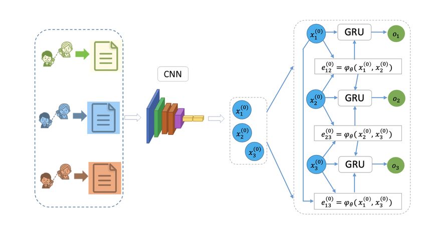
The call transcripts are then used as input to our model to predict RSI. The other meta-data is used for other business-
related insights. As shown in Figure 5, we have development and production clusters. The development cluster is
used to analyze and create insights from the data as well as to train and create predictive models. The models that are
created in this cluster are tested and then deployed to a production cluster for daily scoring. Once a day, a batch script
is run to score all the calls that were received that day. The resulting predicted scores are stored in a database for the
business to consume them. These generated predictions are used for different purposes as: agent education/feedback,
process improvement, and other use-cases that help the company to serve its customers more efficiently. For many of
this tasks being able to identify low scoring calls with high precision is paramount to optimize utilization of resources
and managers’ time.
6 Related Work
Research studies on emotion recognition using human-human real-life corpus extracted from call center calls are limited.
In [22] a system for emotion recognition in the call center domain is proposed. The goal was to classify parts of dialogs
into different emotional states.
Park and Gates [23] developed a method to automatically measure customer satisfaction by analyzing call transcripts in
near real-time. They built machine learning models that predict the degree of customer satisfaction in a scale from 1 to
5 with an accuracy of 66%. Sun et al. [24] adopted a different approach, based on fusion techniques, to predict the user
emotional state from dialogs extracted from a Chinese Mobile call center corpus.
Recently, convolutional neural networks have been used on raw audio signals for prediction of self-reported customer
satisfaction from call center[25]. They pretraining a network on debates from TV shows . Then, the last layers of the
network are fine-tuned with more than 18000 conversations from several call centers. The CNN-based system achieved
comparable performance to the systems based on traditional hand-designed features.
9A PREPRINT - F EBRUARY 9, 2021
Figure 5: Architecture overview of our deployed system
Emotion recognition in the call center domain usually involves rating based on an ordinal scale. Indeed, psychometric
studies show that human ratings of emotion do not follow an absolute scale [26].
There are several algorithms which specifically benefit from the ordering information and yield better performance than
nominal classification and regression approaches. There are algorithms that focus on comparing training examples
in a pairwise manner using binary linear classifiers [27, 28]. Crammer and Singer [29] developed an ordinal ranking
algorithm based on the online perceptron algorithm with multiple thresholds.
Some areas where ordinal ranking problems are found include medical research [30], brain computer interface [31],
credit rating [32], facial beauty assessment [33], image classification [34], and more. All these works are examples of
applications of ordinal ranking models, where exploiting ordering information improves their performance with respect
to their nominal counterparts.
The concept of graph neural network (GNN) was first proposed in [35], which extended existing neural networks for
learning with data and domains that benefit for being represented in graph domains. Generally, in a GNN, each node is
influenced by its features and the related nodes to it (neighbors). This framework fits naturally to the problem of ordinal
ranking where the ordering relations can be represented by edges in a graph. There are prior applications of GNN to the
ranking problem. For example in [36] a GNN is used to rank attacks in network security setting. A comprehensive very
recent survey on GNNs and their applications is presented in [20].
7 Conclusions
This paper describes an efficient updated system for predicting self-reported satisfaction scores of customer phone
calls. Our system has been implemented into a production pipeline that is currently predicting caller satisfaction of
approximately 30,000 incoming calls each business day and generating frequent reports read by call-center managers
and decision makers in our company to potentially improve processes that impact daily customer interactions.
In this work, we described a newly implemented learning algorithm based on GNNs that has considerably improved our
system accuracy and that can be generalized to other ranking tasks inside and outside the customer satisfaction and the
insurance domain.
We presented empirical evaluation based on a large number of real customers calls that shows that this approach
yields more accurate satisfaction predictions than standard regression and ranking models while only using raw call
speech-to-text transcriptions.
We are excited to report that post-deployment validation of our system indicates that the average satisfaction prediction
for groups of calls agrees very strongly with actual satisfaction scores, especially for large groups.
10A PREPRINT - F EBRUARY 9, 2021
As future work, We are interested in human-in-the-loop / active learning approaches where a feedback loop can be used
to improve the system as it is used. Under this paradigm, restricting supervision to paired comparisons can be tedious
and wasteful due to the quadratic nature of possible comparisons. Instead we could present the oracle with the task of
ordering a small subset of examples at the time, which could result in a more streamlined experience for the labeler and
more efficient way to capture feedback.
References
[1] Kathryn Woods. Exploring the relationship between employee turnover rate and customer satisfaction levels. The
Exchange, SSRN, 2015.
[2] Joseph Bockhorst, Shi Yu, Luisa Polania, and Glenn Fung. Predicting self-reported customer satisfaction of
interactions with a corporate call center. In Joint European Conference on Machine Learning and Knowledge
Discovery in Databases, pages 179–190. Springer, 2017.
[3] Zihang Meng, Nagesh Adluru, Hyunwoo J Kim, Glenn Fung, and Vikas Singh. Efficient relative attribute learning
using graph neural networks. In Proceedings of the European Conference on Computer Vision (ECCV), pages
552–567, 2018.
[4] Richard L Dykstra. An isotonic regression algorithm. Journal of Statistical Planning and Inference, 5(4):355–363,
1981.
[5] Justin Gilmer, Samuel S Schoenholz, Patrick F Riley, Oriol Vinyals, and George E Dahl. Neural message passing
for quantum chemistry. arXiv preprint arXiv:1704.01212, 2017.
[6] Chris Burges, Tal Shaked, Erin Renshaw, Ari Lazier, Matt Deeds, Nicole Hamilton, and Greg Hullender. Learning
to rank using gradient descent. In Proceedings of the 22nd international conference on Machine learning, pages
89–96. ACM, 2005.
[7] Yaser Souri, Erfan Noury, and Ehsan Adeli. Deep relative attributes. In Asian Conference on Computer Vision,
pages 118–133. Springer, 2016.
[8] Krishna Kumar Singh and Yong Jae Lee. End-to-end localization and ranking for relative attributes. In European
Conference on Computer Vision, pages 753–769. Springer, 2016.
[9] Yoon Kim. Convolutional neural networks for sentence classification. arXiv preprint arXiv:1408.5882, 2014.
[10] Ruining He and Julian McAuley. Ups and downs: Modeling the visual evolution of fashion trends with one-class
collaborative filtering. In proceedings of the 25th international conference on world wide web, pages 507–517,
2016.
[11] Julian McAuley, Christopher Targett, Qinfeng Shi, and Anton Van Den Hengel. Image-based recommendations
on styles and substitutes. In Proceedings of the 38th international ACM SIGIR conference on research and
development in information retrieval, pages 43–52, 2015.
[12] Armand Joulin, Edouard Grave, Piotr Bojanowski, and Tomas Mikolov. Bag of tricks for efficient text classification.
In Proceedings of the 15th Conference of the European Chapter of the Association for Computational Linguistics:
Volume 2, Short Papers, pages 427–431. Association for Computational Linguistics, April 2017.
[13] Jeffrey Pennington, Richard Socher, and Christopher D Manning. Glove: Global vectors for word representation.
In Proceedings of the 2014 conference on empirical methods in natural language processing (EMNLP), pages
1532–1543, 2014.
[14] Daniel Cer, Yinfei Yang, Sheng-yi Kong, Nan Hua, Nicole Limtiaco, Rhomni St John, Noah Constant, Mario
Guajardo-Cespedes, Steve Yuan, Chris Tar, et al. Universal sentence encoder. arXiv preprint arXiv:1803.11175,
2018.
[15] Robert Tibshirani. Regression shrinkage and selection via the lasso. Journal of the Royal Statistical Society. Series
B (Methodological), pages 267–288, 1996.
[16] Thomas Zimmermann, Rahul Premraj, and Andreas Zeller. Predicting defects for eclipse. In Predictor Models in
Software Engineering, 2007. PROMISE’07: ICSE Workshops 2007. International Workshop on, pages 9–9. IEEE,
2007.
[17] Kalervo Järvelin and Jaana Kekäläinen. Ir evaluation methods for retrieving highly relevant documents. In ACM
SIGIR Forum, volume 51, pages 243–250. ACM New York, NY, USA, 2017.
[18] Diederik P Kingma and Jimmy Ba. Adam: A method for stochastic optimization. arXiv preprint arXiv:1412.6980,
2014.
11A PREPRINT - F EBRUARY 9, 2021
[19] Xavier Glorot and Yoshua Bengio. Understanding the difficulty of training deep feedforward neural networks.
In Proceedings of the thirteenth international conference on artificial intelligence and statistics, pages 249–256,
2010.
[20] Jie Zhou, Ganqu Cui, Zhengyan Zhang, Cheng Yang, Zhiyuan Liu, and Maosong Sun. Graph neural networks: A
review of methods and applications. CoRR, abs/1812.08434, 2018.
[21] Xue Mao, Zhouyu Fu, Ou Wu, and Weiming Hu. Optimizing locally linear classifiers with supervised anchor
point learning. In IJCAI, 2015.
[22] C. Vaudable and L. Devillers. Negative emotions detection as an indicator of dialogs quality in call centers. In
IEEE International Conference on Acoustics, Speech and Signal Processing (ICASSP), pages 5109–5112, 2012.
[23] Y. Park and S.C. Gates. Towards real-time measurement of customer satisfaction using automatically generated
call transcripts. In Proceedings of the 18th ACM conference on Information and knowledge management, pages
1387–1396. ACM, 2009.
[24] J. Sun, W. Xu, Y. Yan, C. Wang, Z. Ren, P. Cong, H. Wang, and J. Feng. Information fusion in automatic user
satisfaction analysis in call center. In International Conference on Intelligent Human-Machine Systems and
Cybernetics (IHMSC), volume 1, pages 425–428, 2016.
[25] C. Segura, D. Balcells, M. Umbert, J. Arias, and J. Luque. Automatic speech feature learning for continuous
prediction of customer satisfaction in contact center phone calls. In Advances in Speech and Language Technologies
for Iberian Languages: Third International Conference, IberSPEECH 2016, Lisbon, Portugal, November 23-25,
2016, pages 255–265. Springer, 2016.
[26] A. Metallinou and S. Narayanan. Annotation and processing of continuous emotional attributes: Challenges and
opportunities. In IEEE International Conference and Workshops on Automatic Face and Gesture Recognition,
pages 1–8, 2013.
[27] R. Herbrich, T. Graepel, and K. Obermayer. Large margin rank boundaries for ordinal regression. Advances in
neural information processing systems, pages 115–132, 1999.
[28] S. Har-Peled, D. Roth, and D. Zimak. Constraint classification: A new approach to multiclass classification. In
International Conference on Algorithmic Learning Theory, pages 365–379. Springer, 2002.
[29] K. Crammer and Y. Singer. Online ranking by projecting. Neural Computation, 17(1):145–175, 2005.
[30] M. Pérez-Ortiz, M. Cruz-Ramírez, M.D. Ayllón-Terán, N. Heaton, R. Ciria, and C. Hervás-Martínez. An organ
allocation system for liver transplantation based on ordinal regression. Applied Soft Computing, 14:88–98, 2014.
[31] J.W. Yoon, S.J. Roberts, M. Dyson, and J.Q. Gan. Bayesian inference for an adaptive Ordered Probit model: An
application to brain computer interfacing. Neural Networks, 24(7):726–734, 2011.
[32] K. Kim and H. Ahn. A corporate credit rating model using multiclass support vector machines with an ordinal
pairwise partitioning approach. Computers and Operations Research, 39(8):1800–1811, 2012.
[33] H. Yan. Cost-sensitive ordinal regression for fully automatic facial beauty assessment. Neurocomputing, 129:334–
342, 2014.
[34] Q. Tian, S. Chen, and X. Tan. Comparative study among three strategies of incorporating spatial structures to
ordinal image regression. Neurocomputing, 136:152–161, 2014.
[35] Franco Scarselli, Marco Gori, Ah Chung Tsoi, Markus Hagenbuchner, and Gabriele Monfardini. The graph neural
network model. Trans. Neur. Netw., 20(1), January 2009.
[36] Liang Lu, Reihaneh Safavi-Naini, Markus Hagenbuchner, Willy Susilo, Jeffrey Horton, Sweah Liang Yong, and
Ah Chung Tsoi. Ranking attack graphs with graph neural networks. In ISPEC 2009, 2009.
12You can also read