Can seafloor voltage cables be used to study large-scale circulation? An investigation in the Pacific Ocean
←
→
Page content transcription
If your browser does not render page correctly, please read the page content below
Ocean Sci., 17, 383–392, 2021
https://doi.org/10.5194/os-17-383-2021
© Author(s) 2021. This work is distributed under
the Creative Commons Attribution 4.0 License.

Can seafloor voltage cables be used to study large-scale circulation?
An investigation in the Pacific Ocean
Jakub Velímský1 , Neesha R. Schnepf2,3 , Manoj C. Nair2,3 , and Natalie P. Thomas4
1 Department of Geophysics, Faculty of Mathematics and Physics, Charles University, Prague, Czech Republic
2 Cooperative Institute for Research in Environmental Sciences (CIRES), University of Colorado, Boulder, CO, USA
3 National Centers for Environmental Information, National Oceanic and Atmospheric Administration, Boulder, CO, USA
4 Department of Atmospheric and Oceanic Science, University of Maryland, College Park, MD, USA

Correspondence: Jakub Velímský (jakub.velimsky@mff.cuni.cz)

Received: 16 December 2019 – Discussion started: 24 January 2020
Revised: 17 January 2021 – Accepted: 18 January 2021 – Published: 22 February 2021

Abstract. Marine electromagnetic (EM) signals largely de-         voltage cables can be used to study large-scale circulation
pend on three factors: flow velocity, Earth’s main magnetic       may eventually be yes.
field, and seawater’s electrical conductivity (which depends
on the local temperature and salinity). Because of this, there
has been recent interest in using marine EM signals to mon-
itor and study ocean circulation. Our study utilizes voltage      1   Introduction
data from retired seafloor telecommunication cables in the
Pacific Ocean to examine whether such cables could be used        Evaluating and predicting the ocean state is crucially im-
to monitor circulation velocity or transport on large oceanic     portant for reconciling and mitigating the impact of climate
scales. We process the cable data to isolate the seasonal and     change on our planet. Oceanic electromagnetic (EM) signals
monthly variations and then evaluate the correlation between      may be directly related to physical parameters of the ocean
the processed data and numerical predictions of the electric      state, including flow velocity, temperature, and salinity. This
field induced by an estimate of ocean circulation. We find        has been known for centuries: in 1832, Michael Faraday was
that the correlation between cable voltage data and numeri-       the first to attempt an experiment of measuring the voltage
cal predictions strongly depends on both the strength and co-     induced by the brackish water of the Thames River (Faraday,
herence of the model velocities flowing across the cable, the     1832). His study was inconclusive, but since then, marine
local EM environment, as well as the length of the cable. The     EM signals have been detected by both ground and satellite
cable within the Kuroshio Current had good correlation be-        measurements (Larsen, 1968; Malin, 1970; Sanford, 1971;
tween data and predictions, whereas two of the cables in the      Cox et al., 1971; Tyler et al., 2003; Sabaka et al., 2016).
Eastern Pacific Gyre – a region with both low flow speeds and        Marine electromagnetic fields are produced because saline
interfering velocity directions across the cable – did not have   ocean water is a conducting fluid with a mean electrical con-
any clear correlation between data and predictions. Mean-         ductivity of σ = 3–4 S m−1 . As this electrically conductive
while, a third cable also located in the Eastern Pacific Gyre     fluid passes through Earth’s main magnetic field (| F | ≈ 20–
showed good correlation between data and predictions – al-        70 µT), it induces electric fields, electric currents, and sec-
though the cable is very long and the speeds were low, it         ondary magnetic fields. The electric current produced by
was located in a region of coherent flow velocity across the      a specific oceanic flow depends on the flow’s velocity, the
cable. While much improvement is needed before utilizing          Earth’s main magnetic field, and the seawater electrical con-
seafloor voltage cables to study and monitor oceanic circu-       ductivity, which in turn depends on salinity and temperature.
lation across wide regions, we believe that with additional       Thus, ideally, three physical oceanic parameters could be ex-
work, the answer to the question of whether or not seafloor       tracted from marine EM studies: velocity, salinity, and tem-
                                                                  perature. However, extracting multiple parameters would re-

Published by Copernicus Publications on behalf of the European Geosciences Union.
384 J. Velímský et al.: Investigating seafloor voltage cables’ transport signals
quire using multiple oceanic electromagnetic signals (e.g.,
the signals from multiple tidal modes and perhaps also from
circulation) (Irrgang et al., 2017; Schnepf, 2017).
In practice, velocity is the only quantity so far deter-
minable from marine EM data. This was accomplished using
a passive seafloor telecommunications cable which recorded
the voltage difference between Florida and Grand Bahama
Island, a distance of approximately 200 km (Larsen and San-
ford, 1985; Spain and Sanford, 1987; Larsen, 1991, 1992;
Baringer and Larsen, 2001). As the Florida Current passed
over the cable, a voltage was induced, and this voltage was
directly related to the depth-integrated velocity across the
cable (i.e., they determined the transport volume). Since
1985, the National Oceanic and Atmospheric Administra-
tion (NOAA) has been using submarine cables to monitor the
transport of the Florida Current through the Straits of Florida
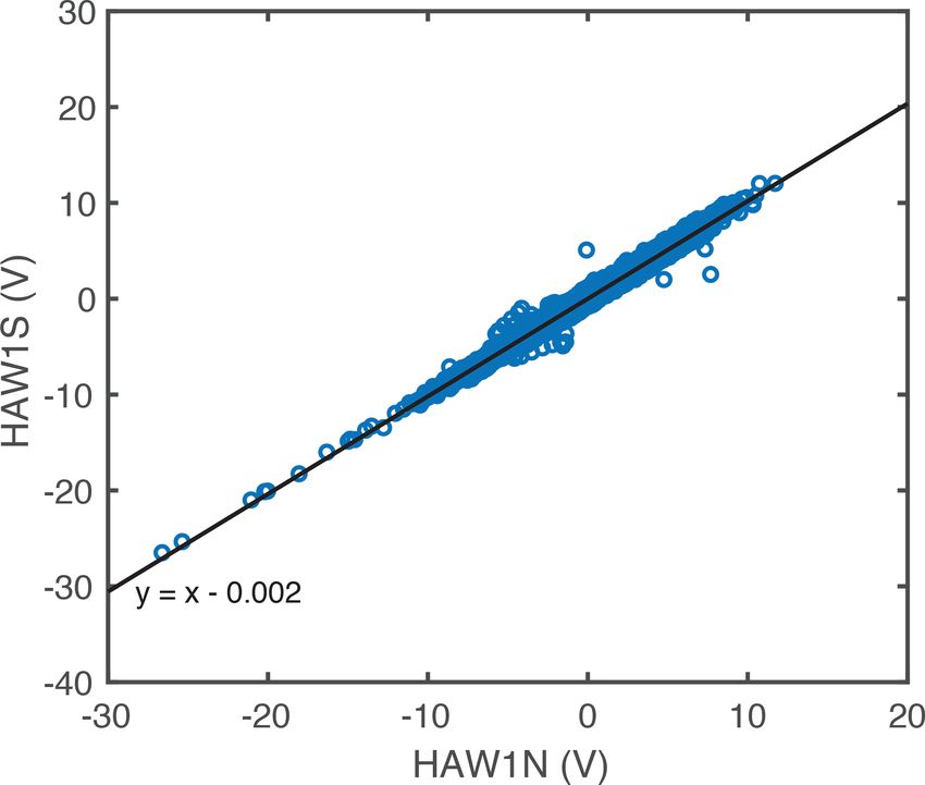
(Meinen et al., 2020). Figure 1. The voltage data of HAW1N versus HAW1S are shown
While data from seafloor voltage cables have been used in a correlation scatterplot. As shown by the line of best fit (y =
to study a variety of geopotential fields (Lanzerotti et al., x − 0.002), the data from the two cables match very closely.
1986, 1992a; Chave et al., 1992; Shimizu et al., 1998; Fu-
jii and Utada, 2000; Lanzerotti et al., 2001), NOAA’s work
in the Straits of Florida is the only case of a seafloor volt- 2 Data and data processing
age cable being reliable to determine the overlying oceanic
flow. Numerical work suggests that cables spanning larger re- This study used hourly data from four seafloor voltage ca-
gions should still strongly correlate with the flow velocities bles (detailed in Table 1): three retired AT&T cables (the
(Flosadóttir et al., 1997; Vanyan et al., 1998; Manoj et al., HAW cables) and one cable managed by the University of
2010); however, there are many challenges in using longer Tokyo’s Earthquake Research Institute (the OKI cable). The
cables. These challenges are largely due to the myriad of pro- HAW1N and HAW1S cables are 3805 km long and run par-
cesses which may also induce marine electromagnetic fields, allel to each other from Point Arena, California, to Hanauma
especially across the length of the cable, such as secular vari- Bay, Hawaii. As shown in Fig. 1, the parallel cables have
ation (Shimizu et al., 1998), variations in ionospheric tides very similar data, providing a unique and helpful situation
(Pedatella et al., 2012; Schnepf et al., 2018), geomagnetic for testing the data processing methods and for comparing
storms, or longer period ionospheric and magnetospheric sig- the observations to numerical predictions. These three cables
nals (Lanzerotti et al., 1992a, 1995, 2001). Additionally, be- have been used in previous studies, including those exam-
cause the cable voltage is produced from the electric field in- ining geopotential variations (Chave et al., 1992; Lanzerotti
tegrated along the entire cable length, the longer the cable is, et al., 1992b; Fujii and Utada, 2000), ionospheric phenom-
the more challenging it is to decompose the total contribution ena (Lanzerotti et al., 1992a), oceanic tides (Fujii and Utada,
to the cross-cable ocean transport in any particular section of 2000), and electrical conductivity of the lithosphere and the
the cable. mantle (Koyama, 2001).
This study aims to provide a “first step” answer to the fol- The first step in processing the hourly data was the removal
lowing question: can seafloor voltage cables be used to study of geomagnetically noisy days (i.e., days where the geomag-
large-scale circulation? To investigate whether it may even- netic Ap index was greater than or equal to 20; see Denig,
tually be feasible to use large-scale voltage cables for moni- 2015 for more on the Ap index). In this way, we reduce
toring ocean flows, we evaluate the correlation between data the contribution from magnetic field variations of magneto-
from large-scale seafloor voltage cables and numerical pre- spheric origin and their induced counterparts. This shrunk
dictions of the electric field induced by 3-D ocean circula- the amount of available data by 16.1 %–21.6 % for each ca-
tion velocity fields. While this work builds on studies using ble. Further reduction of the datasets by using only night-side
seafloor voltage cables to monitor flow velocity in ∼ 100 km data is impossible for the HAW cables, which span multi-
wide passages, this study aims to examine this application in ple time zones, and impractical for the OKI cable due to a
basin-wide seafloor voltage cables. significant decrease in the dataset size and increase in vari-
ance. Next, to remove tidal signals, the 12 dominant daily
tidal modes were fit to the data via least squares and then
subtracted. The following tidal periods were used: 4 (S6 ),
4.8 (S5 ), 6 (S4 ), 8 (S3 ), 11.967236 (K2 ), 12 (S2 ), 12.421
(M2 ), 12.6583 (N2 ), 23.934472 (K1 ), 24 (S1 ), 24.066 (P1 ),
Ocean Sci., 17, 383–392, 2021 https://doi.org/10.5194/os-17-383-2021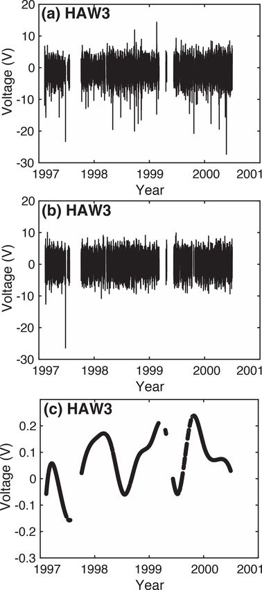
J. Velímský et al.: Investigating seafloor voltage cables’ transport signals                                                      385

Table 1. The seafloor voltage cables used in this study. The HAW1N and HAW1S cables run parallel to each other.

         Cable                    Starting location            Ending location            Length (km)              Time span
         HAW1N and HAW1S          Point Arena, CA, USA         Hanauma Bay, HI, USA              3805    Apr 1990–Dec 2001
         HAW3                     San Luis Obispo, CA, USA     Makaha, HI, USA                   3946    Aug 1994–Jul 2000
         OKI                      Ninomiya, Honshu, Japan      Okinawa, Japan                    1447    Apr 1999–Dec 2001

and 25.891 h (O1 ). Because the datasets have many gaps ex-
ceeding 24 h in length (for example, see Fig. 2), bandpass
filtering was not used. The data were then smoothed using
cubic splines. For seasonal variations, we used 90 d knots
between splines, and for monthly variations, we used 30.5 d
between knots. Although the daily variations should directly
relate to barotropic wind-forced processes (Irrgang et al.,
2016a, b, 2017), because of both the data’s hourly time sam-
pling and frequent data gaps, as well as challenges in pro-
ducing daily numerical predictions, we chose to focus on
monthly and seasonal variations. Each step of the data pro-
cessing is shown in Fig. 2. As the final step, the mean value
is removed from all time series.
    A weakness of this data processing is that it does not pre-
vent the inclusion of induced signals due to seasonal changes
in ionospheric electromagnetic tidal strength. While we re-
moved tidal signals from a least-squares fit, we applied this
fit to the entire dataset and did not attempt to remove seasonal
changes in ionospheric tides. Seasonally, ionospheric tides
can significantly change amplitude (Pedatella et al., 2012),
and the horizontal components of these tides are likely to in-
duce signals at the ground (Schnepf et al., 2018), however,
attempting to constrain seasonal changes in tidal strength is
challenging. Ideally, the least-squares fit could be conducted
on shorter intervals of the data, but this worsens the accuracy
of the least-squares inversion. Ionospheric field models could
be used, but this would also introduce unknown error quan-
tities. Thus, we did not attempt to remove seasonal changes
in tidal amplitude but remind the reader that these signals           Figure 2. Each step of the data processing is shown here using
                                                                      HAW3 as an example: (a) the raw time series, (b) the time se-
may influence the monthly and seasonal variations. The con-
                                                                      ries with days of Ap > 20 removed and tidal signals also removed,
tribution of the main field secular variation is not removed          and (c) the smoothed time series produced by splines with 90 d
from the data, as it is included in the numerical calculations        knots.
described in the next section.

                                                                      Here, B(r; t) is the induced magnetic field, u(r; t) is the ve-
                                                                      locity, µ0 is the magnetic permeability of vacuum, σ (r; t) is
3    Numerical predictions of the ocean circulation’s
                                                                      the electrical conductivity, and F (r; t) is the main geomag-
     electric field
                                                                      netic field. The observable electric field E(r; t) is obtained
                                                                      from the induced magnetic field by post-processing,
We numerically predict the electromagnetic signals produced
by ocean circulation using the ElmgTD time-domain numer-                     1
ical solver of the electromagnetic induction equation (Velím-         E=         (∇ × B) − u × F .                                 (2)
                                                                            µ0 σ
ský and Martinec, 2005; Velímský, 2013; Šachl et al., 2019;
Velímský et al., 2019):                                                 The ElmgTD time-domain solver is based on spherical
                                                                      harmonic parameterization in lateral coordinates and uses 1-

     ∂B        1                                                      D finite elements for radial discretization. The model is fully
µ0      +∇ ×     ∇ × B = µ0 ∇ × (u × F ) .                   (1)      3-D, also incorporating the vertical stratification of the ocean
     ∂t        σ

https://doi.org/10.5194/os-17-383-2021                                                               Ocean Sci., 17, 383–392, 2021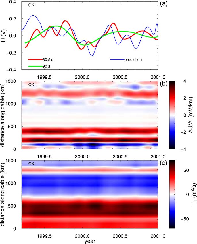
386                                                J. Velímský et al.: Investigating seafloor voltage cables’ transport signals

electrical conductivity and of the velocities as well as ac-       cretization layer. The linear trend was finally removed from
counting for the effect of variable bathymetry. Moreover, the      each time series of predicted cable voltages.
seasonal variations in the ocean electrical conductivity and
the secular variations in the main field are taken into account.
The solution includes both the poloidal and toroidal compo-        4   Results and discussion
nents of the induced magnetic field (Šachl et al., 2019; Velím-
ský et al., 2019), thereby allowing for the inductive and gal-     Figures 4, 5, and 6 summarize the processed voltages and
vanic coupling between the oceans and the mantle as well as        their numerical predictions from the ElmgTD ECCO-based
self-induction within the oceans. Numerically, the linear sys-     simulation for individual cables. Panel a in each figure shows
tem is solved by the preconditioned iterative BiCGStab(2)          the time series of cable voltages processed with the 90 d knot-
scheme (Sleijpen and Fokkema, 1993) with massive paral-            ted spline fit and the 30.5 d knotted spline fit in red and green,
lelization applied across the time levels.                         respectively. In the case of the HAW1 cables, the HAW1N
   Monthly values of the horizontal and vertical components        and HAW1S branches are distinguished by solid and dashed
of ocean velocity from the data-assimilated Estimating the         lines, respectively, and the blue line shows the results of the
Circulation and Climate of the Ocean (ECCOv4r4) (Forget            numerical predictions. A linear trend was removed from all
et al., 2015; Fukumori et al., 2017) model were input into the     shown time series. Panel b in Figs. 4, 5, and 6 shows the nu-
ElmgTD solver to compute the electromagnetic fields that           merical predictions of the voltage gradient (i.e., the electric
they induce from January 1997 to November 2001. Along              field) on the seafloor, along the respective cables, before inte-
with the monthly velocity values from ECCO, monthly val-           gration. Finally, panel c in Figs. 4, 5, and 6 displays the trans-
ues from the International Geomagnetic Reference Field             port T⊥ of the ECCO model across each cable. Note that by
(IGRF) (Finlay et al., 2010) were used for the main field,         transport in this context we denote the vertically integrated
and monthly climatological data from NOAA’s World Ocean            velocity component perpendicular to the cable for each ca-
Atlas (WOA) were used to describe the global seawater elec-        ble element position and time (hence the unit of m2 s−1 ).
trical conductivity σ (Tyler et al., 2017). The conductivity       Although it is not a direct input to the numerical simula-
model also includes the coastal and ocean sediments on the         tions (contrary to the velocities in individual ECCO layers),
seafloor with thickness distribution and conductivity values       it serves as a useful proxy for discussions below.
following Everett et al. (2003).                                      Looking first at the common features of the results for all
   Figure 3 illustrates these inputs used for the ElmgTD nu-       cables, we note, as expected from basic geometrical consid-
merical solver. The vertical velocity is not shown here; al-       erations, a general similarity between the voltage gradient
though it is included in our calculations, as it represents only   along the cable and the water transport across the cable T⊥ .
a minimum additional computational burden, its effect on           We can use these to discuss the effect of individual currents
the induced fields is negligible. Underlying these inputs, the     on the numerical predictions. However, while the ocean flows
electrical conductivity of the mantle follows the 1-D global       are certainly the dominant term controlling the induced elec-
profile obtained by the inversion of satellite data (Grayver       tric fields, the additional contributions of other effects yield
et al., 2017).                                                     a much richer spatiotemporal structure. The main field vari-
   In the present calculations, we truncate the spherical har-     ations in both space and time can have a linear impact on the
monic expansion at degree 240, corresponding to approxi-           large-scale features, as implied by the forcing term of the EM
mately 0.75◦ × 0.75◦ resolution. The radial parameterization       induction Eq. (1). Moreover, the local variations in seawater
within the oceans uses 50 shell layers, following the irregu-      conductivity, the bathymetry, and the sediment thickness af-
lar discretization of the ECCO model. The seawater monthly         fect the electric field in a non-linear way. In particular, the
conductivities from NOAA’s WOA were interpolated to the            toroidal magnetic mode, which corresponds to the poloidal
same grid via bilinear formula in angular coordinates and          electric currents and stems from the galvanic coupling be-
weighted averaging in radial coordinate, which preserves the       tween the ocean and the underlying solid Earth, can play an
total conductance.                                                 important role (Chave et al., 1989; Velímský et al., 2019).
   The model was run from January 1997 through to the                 Upon closer inspection of the OKI cable results, the im-
end of November 2001. Global results were extracted from           portance of the Kuroshio Current stands out, at the distance
the middle of every month (e.g., 17 January, 15 February,          of 300–600 km from Honshu (Fig. 4c). It produces the largest
18 March, and 17 April 1997), but daily results were ex-           contribution to the predicted voltages by far (Fig. 4a, b). In
tracted along the transect of the cables’ paths.                   terms of spatial distribution, the positions along the cable
   To compare numerical predictions with the processed             where the largest contributions to the electric field are in-
seafloor cable observations, the electric field was integrated     duced do not match with the peak positions of the cross-cable
along the seafloor between the endpoints of each cable. For        transport. This discrepancy can be attributed to the electri-
each cable element, the electric field component along the         cally strongly heterogeneous environment caused by large
cable direction was calculated in the lowermost ocean dis-         bathymetry changes in the vicinity of the Ryukyu arc. The
                                                                   ECCO model suggests an increase in the transport in the last

Ocean Sci., 17, 383–392, 2021                                                           https://doi.org/10.5194/os-17-383-2021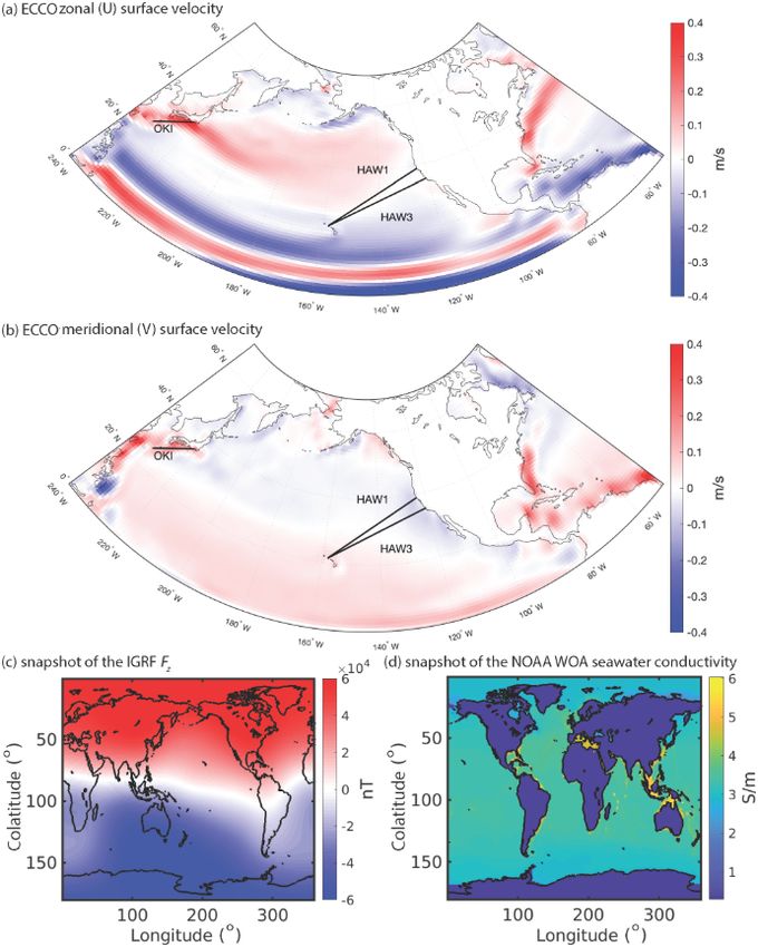
J. Velímský et al.: Investigating seafloor voltage cables’ transport signals                                                              387

Figure 3. The surface velocities from ECCO are shown (a) for the zonal (U ) component and (b) for the meridional (V ) component. The
labeled, thick black lines denote the seafloor voltage cables used in this study. A snapshot of the IGRF vertical main field, Fz , from 17 Jan-
uary 1997 is illustrated in panel (c), and panel (d) depicts the NOAA World Ocean Atlas seawater electrical conductivity’s January climatol-
ogy in the surface layer.

months of 2000, which is consequently responsible for the                 and the induced voltages is in good agreement due to an un-
increased voltage in the numerical model. However, no such                complicated electrical conductivity distribution in the deep
increase is present in the observed voltages, and this discrep-           ocean. The ocean transports across the HAW1 cables demon-
ancy remains an open question. If we trust the OKI volt-                  strate larger seasonal variations than in the case of Kuroshio.
ages, it is possible that the ECCO model is overestimating                However, the lack of significant contributions perpendicular
the Kuroshio strength by the end of 2000.                                 to the cable as well as the changing direction of these flows
   In the case of HAW1N and HAW1S, the numerical model                    both along the cable and in time yield poor agreement of the
predicts significantly smaller amplitudes of cable voltage                total integrated voltage with the observations.
variations when compared with the observations (Fig. 5). The                 The HAW3 cable, in contrast, shows good agreement be-
California Current is the main contributor to the total volt-             tween the predicted and observed voltages (Fig. 6). The nu-
ages, at distances up to 1000 km from the Californian coast.              merical model is again dominated by the California Current,
The spatiotemporal distribution of the cross-cable transport              which is here closer to the coast. The HAW3 cable lies a bit

https://doi.org/10.5194/os-17-383-2021                                                                     Ocean Sci., 17, 383–392, 2021
388                                                    J. Velímský et al.: Investigating seafloor voltage cables’ transport signals

Figure 4. The results for the OKI cable. (a) The smoothed time se-      Figure 5. The results for the HAW1 cables. The HAW1N and
ries of cable voltages using 30.5 and 90 d knot separation are shown    HAW1S cables are distinguished by the solid and dashed lines in
in red and green, respectively. The blue line corresponds to the pre-   panel (a). The cable orientation is from California to Hawaii. Oth-
dictions obtained by the numerical model. (b) The time develop-         erwise, the description corresponds to Fig. 4.
ment of the voltage gradient along the cable length from the 3-D
model. In panel (c), we plot the ECCOv4r4 vertically integrated
transport across the cable in a similar way. The cable orientation
follows Table 1, from Honshu to Okinawa.
                                                                        terms of ocean flows. Large correlations were obtained for
                                                                        the HAW1 and HAW3 cable locations, whereas the inte-
                                                                        grated flow across the OKI cable was poorly correlated with
to the south of the HAW1N and HAW1S cables, and it is also              the predicted voltage. This stresses the importance of the ac-
within the low-speed region of the Eastern Pacific Gyre. The            curate modeling of the induced electric field in strongly het-
transport across the cable in the central Pacific is more coher-        erogeneous areas.
ent, yielding slightly stronger signals than in the case of the            In the third column of Table 2, we show the correlation co-
HAW1 cables. Again, the pattern of the cross-cable transport            efficients between the predicted and observed voltages using
is well matched with the spatiotemporal map of the induced              the 30.5 d knot separation datasets. Due to the gaps present
voltages.                                                               in the data, the Gaussian kernel method (Rehfeld et al., 2011)
   In Table 2, we calculated two sets of correlation coeffi-            was applied. It is obvious that the discrepancies between the
cients. In the second column of the table, the voltages pre-            predicted and observed voltages are still large, and significant
dicted by the numerical model were correlated with the total            efforts are required both on the side of data processing and
ECCO-based water transport (in m3 s−1 ) across the respec-              numerical modeling to reconcile the results. The OKI cable
tive cables:                                                            in particular presents an interesting case. Although the to-
                                                                        tal cross-cable transport is less correlated with the predicted
     Zend                                                               voltages than in the case of both HAW1 cables, the agree-
P⊥ =     T⊥ dl.                                                  (3)    ment with the observations is considerably better. This again
      start
                                                                        points to the role of local EM effects.
                                                                           On the side of numerical modeling, one could devise a
These values are independent of the actual cable voltage                comparison study between different ocean models. Indeed,
measurements and can provide an upper limit on what can                 we have used our model to predict the magnetic fields of the
be achieved by the interpretation of long-cable voltages in             LSOMG (Large Scale Ocean Model for Geophysics) model

Ocean Sci., 17, 383–392, 2021                                                                https://doi.org/10.5194/os-17-383-2021
J. Velímský et al.: Investigating seafloor voltage cables’ transport signals 389
here, with 50 ocean layers and spherical harmonic trunca-
tion degree 240, required about 105 CPU hours to complete.
Semi-global or regional modeling tools with local refinement
ability are needed for more accurate numerical studies.
The qualitative comparison of the induced voltages and
water transports along the cables, as presented in this paper,
could be made more exact by applying the principal compo-
nent analysis methodology. When applied only to the water
transports provided by different ocean models, it could re-
duce the burden of calculating a detailed 3-D EM response
to each model and allow a more focused interpretation of the
observed voltages. We plan to carry out such analysis in the
future.
The studies by Larsen (1992) evaluating transport in the
Straits of Florida from seafloor voltage cable data had corre-
lation values corresponding to much higher values than those
of this study. As shown in Fig. 20 of Larsen (1992), the cor-
relation squared values ranged from 0.61 to 0.94. However,
Larsen’s study was fundamentally different: the seafloor volt-
age cable was an order of magnitude shorter than the ca-
bles considered in this study and the Gulf Stream within the
Straits of Florida has large speeds as well as coherent veloci-
ties flowing perpendicularly to the cables. Therefore, overall,
the Larsen (1992) study had a more ideal signal-to-noise ra-
tio.
Figure 6. The results for the HAW3 cable. The cable orientation is
from California to Hawaii. The description corresponds to Fig. 4. 5 Conclusions
Table 2. For individual seafloor cables, we show the correlation We present an evaluation of using seafloor voltage cables
coefficients between the cable voltages predicted by the numerical for monitoring circulation across oceanic basins. We com-
model and the total ECCO-derived water transport across the cable pare processed seafloor voltage cable data with the numer-
P⊥ in the second column. The third column shows the correlation ical predictions produced using an electromagnetic induc-
coefficients between the predicted and observed voltages for 30.5 d
tion solver, fed by flow velocity estimates from the data-
spline knot separation.
assimilated ECCO model and seawater electrical conductiv-
ity climatologies from the NOAA World Ocean Atlas. We
Cable corr (U pred , P⊥ ) corr (U pred , U obs )
find that the correlation between cable voltage data and nu-
HAW1N 0.92 0.28 merical predictions strongly depends on both the amplitude
HAW1S 0.92 0.11 and direction of the flow velocities across the cable.
HAW3 0.78 0.51 Due to the computational constraints, the calculations of
OKI 0.33 0.42 the ocean-induced electric field presented here are limited to
a single realization of ocean velocity estimates: the ECCO
model. Therefore, beside the unmodeled or uncorrected sig-
in the past (Velímský et al., 2019), and we have also at- nals in the seafloor cable voltages, a first-order source of dis-
tempted the calculation of the cable voltages for the eddy- crepancy between the numerical prediction and observation
resolving GLORYS (Global Ocean reanalysis and Simula- is the inaccuracy of the flow velocity estimates. Therefore, an
tion) ocean model (not shown here). One problem related to extended analysis and comparison of the cable voltage calcu-
this approach is the volume of computational resources nec- lations driven by other ocean circulation models is desirable
essary to carry out the calculations. As the cable voltages in the future as well as the consideration of direct velocity
are sensitive to local electric fields, the usual simplifications observations (Szuts et al., 2019).
of the EM induction solver, based on the thin-sheet approx- While much improvement is needed before utilizing
imation, or representing the oceans by a single layer with seafloor voltage cables to study and monitor ocean circula-
integrated water transports and electrical conductances, are tion across large regions, we believe that seafloor voltage
problematic (Šachl et al., 2019; Velímský et al., 2019). The cables can eventually be used to study and monitor large-
single 5-year calculation of the full physical model presented scale ocean flow. The cables used in this study were installed
https://doi.org/10.5194/os-17-383-2021 Ocean Sci., 17, 383–392, 2021390 J. Velímský et al.: Investigating seafloor voltage cables’ transport signals
for telecommunication purposes – there was no regard for the CIRES Innovative Research Program 2017 and the Grant
whether these cables would be best suited to monitor ocean Agency of the Czech Republic (grant no. P210/17-03689S).
currents. Flow information can most reliably be extracted
from seafloor voltage cable data when the flow has mostly
unidirectional, perpendicular velocities across the cable. For Review statement. This paper was edited by Erik van Sebille and
our study, the OKI cable was in the area with the largest reviewed by Zoltan Szuts and one anonymous referee.
velocities, but because it is oriented mostly parallel to the
Kuroshio Current, its correlation would likely greatly im-
prove if it was instead perpendicular to the current’s flow. References
If voltage cables were strategically placed on the seafloor
between Antarctica and Chile (a distance of ∼ 700 km) Baringer, M. O. and Larsen, J. C.: Sixteen years of Florida Current
or between Antarctica and New Zealand (a distance of Transport at 27◦ N, Geophys. Res. Lett., 28, 3179–3182, 2001.
∼ 1300 km), the correlation between data and predictions Chave, A. D., Filloux, J. H., and Luther, D. S.: Electromagnetic in-
could be quite high, due to both the shorter cable length duction by ocean currents: BEMPEX, Phys. Earth Planet. In., 53,
(compared with the HAW1 and HAW3 cables) and the rel- 350–359, https://doi.org/10.1016/0031-9201(89)90021-6, 1989.
Chave, A. D., Luther, D. S., Lanzerotti, L. J., and Medford, L. V.:
atively uniform and large flow velocities. Indeed, seafloor
Geoelectric field measurements on a planetary scale: oceano-
voltage cables may be a very effective method for measur- graphic and geophysical applications, Geophys. Res. Lett., 19,
ing and continuously monitoring the flow of the Antarctic 1411–1414, 1992.
Circumpolar Current – which is definitely something worth Cox, C. S., Filloux, J. H., and Larsen, J. C.: Electromagnetic studies
investigating. of ocean currents and electrical conductivity below the ocean-
Using existing cables, the correlation between data and nu- floor, in: The Sea, Wiley, New York, ISBN: 0674-01732-3, 637–
merical predictions will likely also improve if the method- 693, 1971.
ology is enhanced to remove induced signals from seasonal Denig, W. F.: Geomagnetic kp and ap Indices, available at: http:
variations in ionospheric signals. //www.ngdc.noaa.gov/stp/GEOMAG/kp_ap.html (last access: 15
February 2021), 2015.
Everett, M. E., Constable, S., and Constable, C. G.: Effects of
Data availability. The data and numerical predictions discussed near-surface conductance on global satellite induction responses,
in this study are freely available for download at https://geomag. Geophys. J. Int., 153, 277–286, https://doi.org/10.1046/j.1365-
colorado.edu/OCEM (Velímský et al., 2021). 246X.2003.01906.x, 2003.
Faraday, M.: The Bakerian Lecture, Experimental Re-
searches in Electricity, Terrestrial Magneto-electric
Induction, Philos. T. R. Soc. Lond., 122, 163–194,
Author contributions. NRS and MCN conceived the questions and
https://doi.org/10.1098/rstl.1851.0001, 1832.
methodology of this study and wrote the initial version of the paper.
Finlay, C. C., Maus, S., Beggan, C. D., Bondar, T. N., Chambodut,
NRS and NPT worked on the processing of cable data. MCN super-
A., Chernova, T. A., Chulliat, A., Golovkov, V. P., Hamilton, B.,
vised NRS and NPT on work related to this project and provided
Hamoudi, M., Holme, R., Hulot, G., Kuang, W., Langlais, B.,
useful feedback on improving the paper. JV carried out the numer-
Lesur, V., Lowes, F. J., Lühr, H., Macmillan, S., Mandea, M.,
ical modeling and also contributed to the paper, in particular to the
McLean, S., Manoj, C., Menvielle, M., Michaelis, I., Olsen, N.,
revised version.
Rauberg, J., Rother, M., Sabaka, T. J., Tangborn, A., Tøffner-
Clausen, L., Thébault, E., Thomson, A. W. P., Wardinski, I.,
Wei, Z., and Zvereva, T. I.: International Geomagnetic Reference
Competing interests. The authors declare that they have no conflict Field: the eleventh generation, Geophys. J. Int., 183, 1216–1230,
of interest. https://doi.org/10.1111/j.1365-246X.2010.04804.x, 2010.
Flosadóttir, Á. H., Larsen, J. C., and Smith, J. T.: Motional induc-
tion in North Atlantic circulation models, J. Geophys. Res., 102,
Acknowledgements. The computational resources were provided 10353–10372, 1997.
by the Ministry of Education, Youth and Sport of the Czech Re- Forget, G., Campin, J.-M., Heimbach, P., Hill, C. N., Ponte, R. M.,
public, from the Large Infrastructures for Research, Experimental and Wunsch, C.: ECCO version 4: an integrated framework for
Development and Innovations project “IT4Innovations National Su- non-linear inverse modeling and global ocean state estimation,
percomputing Center – LM2015070” (project ID OPEN-13-21). We Geosci. Model Dev., 8, 3071–3104, https://doi.org/10.5194/gmd-
thank Zoltan Szuts and the anonymous reviewer for their helpful 8-3071-2015, 2015.
comments. Fujii, I. and Utada, H.: On Geoelectric Potential Variations Over
a Planetary Scale, PhD thesis, The University of Tokyo, Tokyo,
Japan, 81 pp., 2000.
Financial support. This research has been supported by the NASA Fukumori, I., Wang, O., Fenty, I., Forget, G., Heimbach,
Earth and Space Science Fellowship (grant no. 80NSSC17K0450), P., and Ponte, R. M.: ECCO version 4, release 3, Tech.
Rep., JPL/Caltech and NASA Physical Oceanography, 10 pp.,
https://doi.org/1721.1/110380, 2017.
Ocean Sci., 17, 383–392, 2021 https://doi.org/10.5194/os-17-383-2021J. Velímský et al.: Investigating seafloor voltage cables’ transport signals 391
Grayver, A. V., Munch, F. D., Kuvshinov, A. V., Khan, A., and Meinen, C. S., Smith, R. H., and Garcia, R. F.: Evalu-
Sabaka, T. J.: Joint inversion of satellite-detected tidal and mag- ating pressure gauges as a potential future replacement
netospheric signals constrains electrical conductivity and water for electromagnetic cable observations of the Florida Cur-
content of the upper mantle and transition zone, Geophys. Res. rent transport at 27◦ N, J. Oper. Oceanogr., 0, 1–11,
Lett., 44, 6074–6081, https://doi.org/10.1002/2017GL073446, https://doi.org/10.1080/1755876X.2020.1780757, 2020.
2017. Pedatella, N. M., Liu, H., and Richmond, A. D.: Atmospheric
Irrgang, C., Saynisch, J., and Thomas, M.: Ensemble simulations of semidiurnal lunar tide climatology simulated by the Whole At-
the magnetic field induced by global ocean circulation: estimat- mosphere Community Climate Model, J. Geophys. Res., 117,
ing the uncertainty, J. Geophys. Res.-Oceans, 121, 1866–1880, A06327, https://doi.org/10.1029/2012JA017792, 2012.
2016a. Rehfeld, K., Marwan, N., Heitzig, J., and Kurths, J.: Compar-
Irrgang, C., Saynisch, J., and Thomas, M.: Impact of variable ison of correlation analysis techniques for irregularly sam-
seawater conductivity on motional induction simulated with pled time series, Nonlin. Processes Geophys., 18, 389–404,
an ocean general circulation model, Ocean Sci., 12, 129–136, https://doi.org/10.5194/npg-18-389-2011, 2011.
https://doi.org/10.5194/os-12-129-2016, 2016b. Sabaka, T. J., Tyler, R. H., and Olsen, N.: Extracting ocean-
Irrgang, C., Saynisch, J., and Thomas, M.: Utilizing oceanic elec- generated tidal magnetic signals from Swarm data through satel-
tromagnetic induction to constrain an ocean general circulation lite gradiometry, Geophys. Res. Lett., 43, 3237–3245, 2016.
model: A data assimilation twin experiment, JAMES, 9, 1703– Šachl, L., Martinec, Z., Velímský, J., Irrgang, C., Petereit, J.,
1720, https://doi.org/10.1002/2017MS000951, 2017. Saynisch, J., Einšpigel, D., and Schnepf, N. R.: Modelling of
Koyama, T.: A study on the electrical conductivity of the mantle by electromagnetic signatures of global ocean circulation: physical
voltage measurements of submarine cables, PhD thesis, Univer- approximations and numerical issues, Earth Planets Space, 71,
sity of Tokyo, Tokyo, Japan, 130 pp., 2001. 58, https://doi.org/10.1186/s40623-019-1033-7, 2019.
Lanzerotti, L. J., Thomson, D. J., Meloni, A., Medford, L. V., and Sanford, T. B.: Motionally induced electric and magnetic
Maclennan, C. G.: Electromagnetic study of the Atlantic conti- fields in the sea, J. Geophys. Res., 76, 3476–3492,
nental margin using a section of a transatlantic cable, J. Geophys. https://doi.org/10.1029/JC076i015p03476, 1971.
Res., 91, 7417–7427, 1986. Schnepf, N. R.: Going electric: Incorporating marine electromag-
Lanzerotti, L. J., Medford, L. V., Kraus, J. S., Maclennan, C. G., and netism into ocean assimilation models, J. Adv. Model. Earth Sy.,
Hunsucker, R. D.: Possible measurements of small-amplitude 9, 1772–1775, https://doi.org/10.1002/2017MS001130, 2017.
TID’s using parallel, unpowered telecommunications cables, Schnepf, N. R., Nair, M., Maute, A., Pedatella, N. M., Ku-
Geophys. Res. Lett., 19, 253–256, 1992a. vshinov, A., and Richmond, A. D.: A Comparison of
Lanzerotti, L. J., Sayres, C. H., Medford, L. V., Kraus, J. S., and Model-Based Ionospheric and Ocean Tidal Magnetic Signals
Maclennan, C. G.: Earth potential over 4000 km between Hawaii With Observatory Data, Geophys. Res. Lett., 45, 7257–7267,
and California, Geophys. Res. Lett., 19, 1177–1180, 1992b. https://doi.org/10.1029/2018GL078487, 2018.
Lanzerotti, L. J., Medford, L. V., Maclennan, C. G., and Shimizu, H., Koyama, T., and Utada, H.: An observational con-
Thomson, D. J.: Studies of Large-Scale Earth Potentials straint on the strength of the toroidal magnetic field at the CMB
Across Oceanic Distances, AT&T Tech. J., 74, 73–84, by time variation of submarine cable voltages, Geophys. Res.
https://doi.org/10.1002/j.1538-7305.1995.tb00185.x, 1995. Lett., 25, 4023–4026, 1998.
Lanzerotti, L. J., Medford, L. V., Maclennan, C. G., Kraus, J. S., Sleijpen, G. L. G. and Fokkema, D. R.: BiCGstab(ell) for Linear
Kappenman, J., and Radasky, W.: Trans-atlantic geopotentials Equations involving Unsymmetric Matrices with Complex Spec-
during the July 2000 solar event and geomagnetic storm, Solar trum, Electron. T. Numer. Ana., 1, 11–32, 1993.
Physics, 204, 351–359, 2001. Spain, P. and Sanford, T. B.: Accurately monitoring the Florida Cur-
Larsen, J. C.: Electric and Magnetic Fields Induced by Deep Sea rent with motionally-induced voltages, J. Mar. Res., 7, 843–870,
Tides, Geophys. J. Roy. Astr. S., 16, 47–70, 1968. 1987.
Larsen, J. C.: Transport measurements from in-service under- Szuts, Z. B., Bower, A. S., Donohue, K. A., Girton, J. B.,
sea telephone cables, IEEE J. Oceanic Eng., 16, 313–318, Hummon, J. M., Katsumata, K., Lumpkin, R., Ortner, P. B.,
https://doi.org/10.1109/48.90893, 1991. Phillips, H. E., Rossby, H. T., Shay, L. K., Sun, C., and Todd,
Larsen, J. C.: Transport and heat flux of the Florida Current at R. E.: The Scientific and Societal Uses of Global Measurements
27◦ N derived from cross-stream voltages and profiling data: the- of Subsurface Velocity, Frontiers in Marine Science, 6, 358,
ory and observations, Philos. T. Roy. Soc. A, 338, 169–236, https://doi.org/10.3389/fmars.2019.00358, 2019.
https://doi.org/10.1098/rsta.1992.0007, 1992. Tyler, R. H., Maus, S., and Lühr, H.: Satellite observations of
Larsen, J. C. and Sanford, T. B.: Florida current volume transports magnetic fields due to ocean tidal flow, Science, 299, 239–241,
from voltage measurements, Science, 227, 302–304, 1985. https://doi.org/10.1126/science.1078074, 2003.
Malin, S. R. C.: Separation of lunar daily geomagnetic variations Tyler, R. H., Boyer, T. P., Minami, T., Zweng, M. M., and Reagan,
into parts of ionospheric and oceanic origin, Geophys. J. Roy. J. R.: Electrical conductivity of the global ocean, Earth Plan-
Astr. S., 21, 447–455, 1970. ets Space, 69, 156, https://doi.org/10.1186/s40623-017-0739-7,
Manoj, C., Kuvshinov, A., Neetu, S., and Harinarayana, T.: Can 2017.
undersea voltage measurements detect tsunamis?, Earth Planets Vanyan, L. L., Utada, H., Shimizu, H., Tanaka, Y., Palshin,
Space, 62, 353–358, https://doi.org/10.5047/eps.2009.10.001, N. A., Stepanov, V., Kouznetsov, V., Medzhitov, R. D., and
2010. Nozdrina, A.: Studies on the lithosphere and the water trans-
port by using the Japan Sea submarine cable (JASC): 1.
https://doi.org/10.5194/os-17-383-2021 Ocean Sci., 17, 383–392, 2021392 J. Velímský et al.: Investigating seafloor voltage cables’ transport signals Theoretical considerations, Earth Planets Space, 50, 35–42, Velímský, J., Šachl, L., and Martinec, Z.: The global toroidal mag- https://doi.org/10.1186/BF03352084, 1998. netic field generated in the Earth’s oceans, Earth Planet. Sc. Lett., Velímský, J.: Determination of three-dimensional distribution of 509, 47–54, https://doi.org/10.1016/j.epsl.2018.12.026, 2019. electrical conductivity in the Earth’s mantle from Swarm satel- Velímský, J., Schnepf, N. R., Nair, M. C., and Thomas, N. P.: lite data: Time-domain approach, Earth Planets Space, 65, 1239– Download Ocean Circulation Electromagnetism (OCEM) Data, 1246, https://doi.org/10.5047/eps.2013.08.001, 2013. available at: https://geomag.colorado.edu/OCEM, last access: 17 Velímský, J. and Martinec, Z.: Time-domain, spherical harmonic- February 2021. finite element approach to transient three-dimensional geo- magnetic induction in a spherical heterogeneous earth, Geo- phys. J. Int., 161, 81–101, https://doi.org/10.1111/j.1365- 246X.2005.02546.x, 2005. Ocean Sci., 17, 383–392, 2021 https://doi.org/10.5194/os-17-383-2021
You can also read