Stochastic reconstruction of spatio-temporal rainfall patterns by inverse hydrologic modelling - HESS
←
→
Page content transcription
If your browser does not render page correctly, please read the page content below
Hydrol. Earth Syst. Sci., 23, 225–237, 2019
https://doi.org/10.5194/hess-23-225-2019
© Author(s) 2019. This work is distributed under
the Creative Commons Attribution 4.0 License.

Stochastic reconstruction of spatio-temporal rainfall patterns by
inverse hydrologic modelling
Jens Grundmann1 , Sebastian Hörning2 , and András Bárdossy3
1 Technische  Universität Dresden, Institute of Hydrology and Meteorology, Dresden, Germany
2 University of Queensland, EAIT, Centre for Coal Seam Gas, Brisbane, Australia
3 Universität Stuttgart, Institute for Modelling Hydraulic and Environmental Systems, Stuttgart, Germany

Correspondence: Jens Grundmann (jens.grundmann@tu-dresden.de)

Received: 25 June 2018 – Discussion started: 2 July 2018
Revised: 19 December 2018 – Accepted: 21 December 2018 – Published: 16 January 2019

Abstract. Knowledge of spatio-temporal rainfall patterns is       real-world study for a flash flood event in a mountainous arid
required as input for distributed hydrologic models used for      region are presented. They underline that knowledge about
tasks such as flood runoff estimation and modelling. Nor-         the spatio-temporal rainfall pattern is crucial for flash flood
mally, these patterns are generated from point observations       modelling even in small catchments and arid and semiarid
on the ground using spatial interpolation methods. However,       environments.
such methods fail in reproducing the true spatio-temporal
rainfall pattern, especially in data-scarce regions with poorly
gauged catchments, or for highly dynamic, small-scale rain-
storms which are not well recorded by existing monitor-           1   Motivation
ing networks. Consequently, uncertainties arise in distributed
rainfall–runoff modelling if poorly identified spatio-temporal    The importance of spatio-temporal rainfall patterns for
rainfall patterns are used, since the amount of rainfall re-      rainfall–runoff (RR) estimation and modelling is well known
ceived by a catchment as well as the dynamics of the runoff       in hydrology and has been addressed by several simula-
generation of flood waves is underestimated. To address           tion studies, especially since distributed hydrologic models
this problem we propose an inverse hydrologic modelling           have become available. Many of those studies demonstrated
approach for stochastic reconstruction of spatio-temporal         the effect of resulting runoff responses for different spatial
rainfall patterns. The methodology combines the stochastic        rainfall patterns (Beven and Hornberger, 1982; Obled et al.,
random field simulator Random Mixing and a distributed            1994; Morin et al., 2006; Nicotina et al., 2008) or addressed
rainfall–runoff model in a Monte Carlo framework. The sim-        the errors in runoff prediction and the difficulties in param-
ulated spatio-temporal rainfall patterns are conditioned on       eterisation and calibration of hydrologic models if the spa-
point rainfall data from ground-based monitoring networks         tially distribution of rainfall is not well known (Troutman,
and the observed hydrograph at the catchment outlet and aim       1983; Lopes, 1996; Chaubey et al., 1999; Andreassian et al.,
to explain measured data at best. Since we infer a three-         2001). As a consequence, studies were performed to inves-
dimensional input variable from an integral catchment re-         tigate configurations of rainfall monitoring networks (Faures
sponse, several candidates for spatio-temporal rainfall pat-      et al., 1995) and rainfall errors and uncertainties for hydro-
terns are feasible and allow for an analysis of their uncer-      logic modelling (McMillan et al., 2011; Renard et al., 2011).
tainty. The methodology is tested on a synthetic rainfall–           In general, rainfall monitoring networks based on point
runoff event on sub-daily time steps and spatial resolution       observations on the ground (station data) require interpo-
of 1 km2 for a catchment partly covered by rainfall. A set        lation methods to obtain spatio-temporal rainfall fields us-
of plausible spatio-temporal rainfall patterns can be obtained    able for distributed hydrologic modelling. Traditional in-
by applying this inverse approach. Furthermore, results of a      terpolation methods fail in reproducing the true spatio-
                                                                  temporal rainfall pattern, especially for (i) data-scarce re-

Published by Copernicus Publications on behalf of the European Geosciences Union.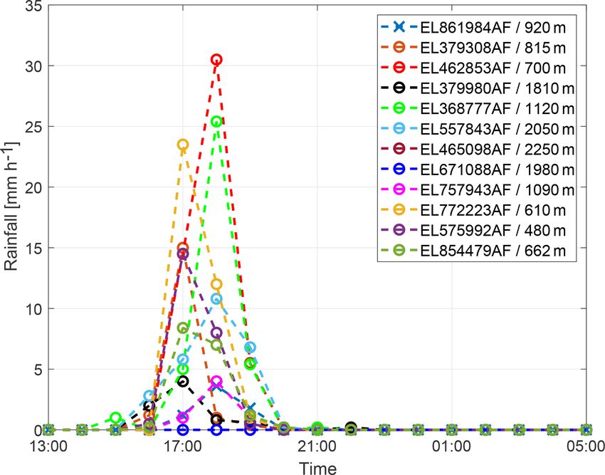
226                                     J. Grundmann et al.: Stochastic reconstruction of spatio-temporal rainfall patterns

gions with poorly gauged catchments and low network den-            patterns (Krajewski et al., 1991; Shah et al., 1996; Casper
sity; (ii) highly dynamic, small-scale rainstorms which are         et al., 2009; Paschalis et al., 2014). However, stochastic rain-
not well recorded by existing monitoring networks; and              fall simulations in combination with distributed hydrologic
(iii) catchments which are partly covered by rainfall. Con-         modelling can be computationally demanding and can fail at
sequently, uncertainties are associated with poorly identi-         matching the observed streamflow if rainfall fields are condi-
fied spatio-temporal rainfall patterns in distributed rainfall–     tioned on rainfall point observations only.
runoff-modelling since the amount of rainfall received by a            On the other hand, inverse hydrologic modelling ap-
catchment as well as the dynamics of runoff generation pro-         proaches have been developed to estimate rainfall time se-
cesses are typically underestimated by current methods.             ries based on observed streamflow data. Those approaches
   The effects of poorly estimated spatio-temporal rainfall         require either an inversion of the underlying mathemati-
fields are visible in particular for semiarid and arid re-          cal equations for the non-linear transfer function (Kirchner,
gions, where rainstorms show a great variability in space and       2009; Kretzschmar et al., 2014) or an application of the hy-
time and the density of ground-based monitoring networks            drologic model in a Bayesian inference scheme (Kavetski
is sparse compared to other regions (Pilgrim et al., 1988).         et al., 2006; Del Giudice et al., 2016). Up to now, both ap-
Based on an analysis of 36 events in a mountainous region           proaches deliver time series of catchment-averaged rainfall
of Oman, McIntyre et al. (2007) show a wide range of event-         only, which gives no idea about the spatial extent and distri-
based runoff coefficients, which underlines that achieving re-      bution of rainfall. This is particularly important when con-
liable runoff predictions by using hydrologic models in those       sidering events such as localised rainstorms, which might be
regions is extremely challenging. This is supported by sev-         underestimated and not accurately portrayed.
eral simulation studies (Al-Qurashi et al., 2008; Bahat et al.,        The goal here is an event-based reconstruction of spatio-
2009), who address the uncertainties in model parameterisa-         temporal rainfall patterns which best explains measured
tion due to uncertain rainfall input. In this context Gunkel        point rainfall data and catchment runoff response. For that
and Lange (2012) report that reliable model parameter esti-         we looked for potential candidates for rainfall fields for sub-
mation was only possible by using rainfall radar. However,          daily time steps and spatial resolution of 1 km2 which, to our
this information is not available everywhere.                       knowledge has not been done so far. To achieve this task, we
   To address the inherent uncertainties described above,           combined stochastic rainfall simulations and distributed hy-
stochastic rainfall generators are used intensively to cre-         drologic modelling in an inverse modelling approach, where
ate spatio-temporal rainfall inputs for distributed hydrologic      spatio-temporal rainfall patterns are conditioned on rainfall
models to transform rainfall into runoff. A large amount of         point observations and observed runoff. The methodology
literature exists describing different approaches for space–        of the inverse hydrologic modelling approach consists of
time simulation of rainfall fields, including multi-site tempo-     the stochastic random field simulator Random Mixing and
ral simulation frameworks (Wilks, 1998), approaches based           a distributed rainfall–runoff model in a Monte Carlo frame-
on the theory of random fields (Bell, 1987; Pegram and              work. Until now, Random Mixing, developed by Bárdossy
Clothier, 2001), or approaches based on the theory of point         and Hörning (2016b) for solving inverse groundwater mod-
processes and its generalisation, which includes the popu-          elling problems, has been used by Haese et al. (2017) for
lar turning-band method (Mantoglou and Wilson, 1982). En-           reconstruction and interpolation of precipitation fields using
hancements were made in order to portray different rainstorm        different data sources for rainfall.
patterns and distinct properties of rainfall fields, like spatial      After this introduction the methods are described in
covariance structure, space–time anomaly, and intermittency         Sect. 2. It gives an overview of the methodology and fur-
(see Leblois and Creutin, 2013; Paschalis et al., 2013; Peleg       ther details for the applied rainfall–runoff model, the Ran-
et al., 2017).                                                      dom Mixing and its application for rainfall fields. Section 3
   Applications of spatio-temporal rainfall simulations to-         aims to test the methodology. A synthetic test site is intro-
gether with hydrologic models are straightforward Monte             duced which is used to demonstrate and discuss (i) the lim-
Carlo types, where a large number of potential rainfall fields      its of common hydrologic modelling approaches (using rain-
are generated driven by stochastic properties of observed           fall interpolation) and (ii) the shortcomings of rainfall sim-
rainstorms or longer time series. These fields are used as          ulations which are not conditioned on the observed runoff.
inputs for distributed hydrologic model simulations to in-          In contrast, the functionality of the inverse hydrologic mod-
vestigate the impact of certain aspects of rainfall like un-        elling approach is illustrated and discussed. In Sect. 4, the
certainty in measured rain depth, spatial variability, etc., on     inverse hydrologic modelling approach is applied for real-
simulated catchment responses. Rainfall simulation applica-         world data by an example of an arid mountainous catchment
tions are performed in unconditional mode (reproducing rain         in Oman. The test site is introduced and results are shown
field statistics only) or conditional mode, where observations      and discussed. Finally, summary and conclusions are given
(e.g. from rain gauges) are reproduced too. The latter are          in Sect. 5.
commonly used for investigating the effect of spatial vari-
ability using fixed total precipitation and variations in spatial

Hydrol. Earth Syst. Sci., 23, 225–237, 2019                                        www.hydrol-earth-syst-sci.net/23/225/2019/
J. Grundmann et al.: Stochastic reconstruction of spatio-temporal rainfall patterns                                                 227

2     Methods                                                     duced by the constant rate fc (x) throughout an event to con-
                                                                  sider infiltration. The calculated effective precipitation (or
2.1    General approach                                           surface runoff) is transferred to the next river channel section
                                                                  considering translation and attenuation processes. Transla-
The methodology described here can be characterized as            tion is accounted for with a grid-based travel-time function
an inverse hydrologic modelling approach. It aims to infer        to include the effects of surface slope and roughness. At-
potential candidates for the unknown spatio-temporal rain-        tenuation is accounted for with a single linear storage unit
fall patterns from runoff observations at the catchment out-      with recession constant fr (x). Both approaches are applied
let, known parameterisation of the rainfall–runoff model,         on grid cells affected by effective precipitation only to fully
and rain gauge observations. The approach combines a grid-        support spatial distributed calculations corresponding to the
based spatially distributed rainfall–runoff model and a con-      spatial extent of the rain field. The properties of several land-
ditional random field simulation technique called Random          scape units are addressed by different parameter sets (for
Mixing (Bárdossy and Hörning, 2016a, b). Random Mix-              Ia (x), fc (x), fr (x)) following the concept of hydrogeologi-
ing is used to simulate a conditional rainfall field which        cal response units (Gerner, 2013) (since hydrologic processes
honours the observed rainfall values as well as their spatial     are mostly driven by hydrogeology in these regions). Runoff
and temporal variability. Afterwards, an optimisation is per-     is routed to the catchment outlet by a simple lag model in
formed to additionally condition the rainfall field on the ob-    combination with a constant rate (ft ) loss model to portray
served runoff. Therefore, the initial field is used as input to   transmission losses along the stream channel. The RR model
the rainfall–runoff model. The deviation between the simu-        is applied on an hourly time step on regular grids cells of
lated runoff and the observed runoff is evaluated based on        1 km by 1 km. Parameters are assumed to be known and fixed
the model efficiency (NSE) defined by Nash and Sutcliffe          during the inverse modelling procedure. The RR model is
(1970). To minimise this deviation the rainfall field is mixed    linked to Random Mixing directly and named with the work-
with another random field which exhibits certain properties       ing title NAMarid.
such that the mixture honours the observed rainfall values
and their spatio-temporal variability. This procedure is re-      2.3   Random Mixing for inverse hydrologic modelling
peated until a satisfying solution, i.e. a conditional rainfall
field that achieves a reasonable NSE, is found. To enable a       Random Mixing is a geostatistical simulation approach. It
reasonable uncertainty estimation the procedure is repeated       uses copulas as spatial random functions (Bárdossy, 2006)
until a predefined number of potential candidates has been        and represents an extension to the gradual deformation ap-
found. In the following, rainfall is used interchangeably with    proach (Hu, 2000). In the following a brief description of the
precipitation.                                                    Random Mixing algorithm is presented. A detailed explana-
                                                                  tion can be found in Hörning (2016).
2.2    Rainfall runoff model                                         The goal of the inverse hydrologic modelling approach
                                                                  presented herein is to find a conditional precipitation field
A simple spatially distributed rainfall–runoff model is used      P (x, t) with location x ∈ D and time t ∈ T which repro-
as transfer function to portray the non-linear transforma-        duces the observed spatial and temporal variability and
tion of spatially distributed rainfall into runoff at catchment   marginal distribution of P . This field should also honour pre-
outlets. The model is dedicated to describe rainfall–runoff       cipitation observations at locations xj and times ti :
processes in arid mountainous regions, which are mostly           P (xj , ti ) = pj, i for j = 1, . . . , J and i = 1, . . . , I,   (1)
based on infiltration excess and Hortonian overland flow. The
model is working on regular grid cells in event-based modes.         Note that P denotes a spatial field and p denotes a pre-
It is parsimonious in the number of parameters, considers         cipitation value within that field. Furthermore, the solution
transmission losses but has no base flow component. Pre-          of a rainfall–runoff model using the field P as input variable
state information at the beginning of an event is neglected       should approximately honour the observed runoff:
since runoff processes mostly start under dry conditions (Pil-    Qt (P ) ≈ qt for t = 1, . . . , T ,                               (2)
grim et al., 1988).
   More specifically, only simple approaches known from           where Qt denotes the rainfall–runoff model and qt represents
hydrologic textbooks for the simulation of single rainfall–       the observed runoff values at time step t. Note that Qt (P )
runoff events (no long-term water balance) are used (Dyck         represents a non-linear function of the field P .
and Peschke, 1983). Effective precipitation Pe(x, t) with lo-        In order to find such a precipitation field P which fulfills
cation x ∈ D and time t ∈ T is calculated by an initial and       the conditions given in Eqs. (1) and (2), Random Mixing can
constant rate loss model applied on each grid cell which is       be applied. Figure 1 shows a flowchart of the corresponding
affected by rainfall. The initial loss Ia (x) represents inter-   procedure.
ception and depression storage. If the accumulated precipi-          Using the given observations pj, i , a marginal distribution
tation exceeds Ia (x) surface runoff may occur, which is re-      G(p) has to be fitted to them. Note that in general any type

www.hydrol-earth-syst-sci.net/23/225/2019/                                          Hydrol. Earth Syst. Sci., 23, 225–237, 2019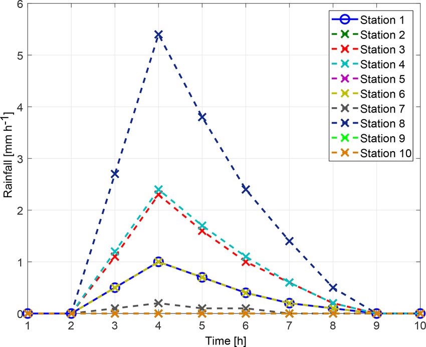
228                                    J. Grundmann et al.: Stochastic reconstruction of spatio-temporal rainfall patterns

Figure 1. Flowchart of the Random Mixing algorithm for inverse hydrologic modelling.

of distribution function (e.g. parametric, non-parametric, and       estimated are p0 and λ. Then, using the fitted marginal dis-
combinations of distributions) can be used. For the applica-         tribution the observed precipitation values are transformed to
tions presented herein the selected marginal distribution con-       standard normal:
sists of two parts: the discrete probability of zero precipita-
                                                                             < 8−1 (p0 )

tion and an exponential distribution for the wet precipitation                                                 if p = 0,
                                                                     w=                                                         (4)
observations. It is defined as follows:                                      8−1 (p0 + p0 (1 − exp(−λp))) otherwise,

             p0                         if p = 0,
G(p) =                                                      (3)      where 8−1 denotes the univariate inverse standard normal
             p0 + p0 (1 − exp(−λp)) otherwise,
                                                                     distribution. Note that zero precipitation observations are not
with p denoting precipitation values, p0 is the discrete proba-      transformed to the same value, but they are considered as in-
bility of zero precipitation and λ denotes the parameter of the      equality constraints as described in Eq. (4). Thus the spatio-
exponential distribution. Thus the parameters that need to be        temporal dependence structure of the variable is taken into

Hydrol. Earth Syst. Sci., 23, 225–237, 2019                                            www.hydrol-earth-syst-sci.net/23/225/2019/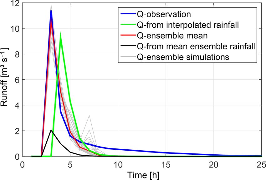
J. Grundmann et al.: Stochastic reconstruction of spatio-temporal rainfall patterns                                            229

                                                                   to obtain a smooth, low-variance field a L2 norm αl2  1
                                                                                                                         P
account as described in Hörning (2016). Further note that
the transformation of the marginal distribution described in       is required. If no such solution is found, an additional field
Eq. (4) can be reversed via the following:                         VL+1 is created, added to the system of linear equation and
                                                                   the system is solved again. Note that with increasing degrees
P (x, t) = G−1 (8(W (x, t))),                               (5)
                                                                   of freedom (i.e. more fields) the L2 norm of the solution de-
where G−1 denotes the inverse marginal distribution of P           creases.
                                                                      Once a solution with an acceptable L2 norm, i.e. αl2
                                                                                                                          P
and 8 denotes the univariate standard normal distribution.
Also, note that W denotes the transformed spatial field while      1 is found the resulting field is defined as follows:
w denotes a transformed observed value within that field.
                                                                          L+M
Note that in this approach we assume that the precipitation               X
                                                                   W∗ =          αl Vl ,                                        (7)
distribution is the same for each location x and each time-
                                                                           l=1
step t. One could use a location and/or time-specific distribu-
tion to take spatial or temporal non-stationarity into account;    where M denotes the number of additional fields added to the
however, this requires a relatively large amount of precipita-     equation system. Note that W ∗ fulfills the conditions defined
tion observations and/or additional information.                   in Eq. (1); however, it does not fulfill Eq. (2) and it does not
   As a next step we assume that the field W is normal, and        represent the correct spatio-temporal dependence structure.
thus its spatio-temporal dependence is described by the nor-          The next step is to simulate fields Uk with k = 1, . . . , K
mal copula with correlation matrix 0 c . In general copulas        which fulfill the homogeneous conditions, i.e. Uk (xj , ti ) =
are multivariate distribution functions defined on the unit hy-    0. Further all fields Uk need to share the same spatio-
percube with uniform univariate marginals. They are used to        temporal dependence structure, again described by 0 c . Such
describe the dependence between random variables indepen-          fields can be generated in a similar way to W ∗ (see Hörning,
dently of their marginal distributions. The normal copula can      2016 for details). The advantage of these fields Uk is that
be derived from a multivariate standard normal distribution        they form a vector space (they are closed for multiplication
(see Bárdossy and Hörning, 2016b, for details). It enables         and addition), thus
modelling of a Gaussian spatio-temporal dependence struc-
ture with arbitrary marginal distribution. Note that its corre-    Wλ = W ∗ + k(λ)(λ1 U1 + . . . + λk Uk ),                     (8)
lation matrix 0 c has to be assessed from the available ob-
servations. If no zero observations are present the maximum        where λk denotes arbitrary weights and k(λ) denotes a scal-
likelihood estimation procedure described in Li (2010) can         ing factor results in a field Wλ , which also fulfills the condi-
be applied to estimate the copula parameters. If zero values       tions prescribed in Eq. (1). The scaling factor is defined as:
are present a modified maximum likelihood approach has to                    s
                                                                                1 − αl2
                                                                                    P
be used (Bárdossy, 2011). It uses a combination of three dif-      k(λ) = ±                                                      (9)
                                                                                  P 2 .
ferent cases (wet–wet pairs, wet–dry pairs, dry–dry pairs of                         λk
observations) for the estimation of the copula parameters.
   As a next step, unconditional standard normal random               It ensures that Wλ exhibits the correct spatio-temporal de-
fields Vl with l = 1, . . . , L are simulated such that they all   pendence structure. Thus, transforming Wλ back to P using
share the same spatio-temporal dependence structure which          Eq. (5) will result in a precipitation field which has the cor-
is described by 0 c of the fitted normal copula. Such fields       rect spatio-temporal dependence structure and marginal dis-
can for example be simulated using fast Fourier transforma-        tribution, and honours the precipitation observations.
tion for regular grids (Wood and Chan, 1994; Wood, 1995;              To also honour the observed runoff defined in Eq. (2) an
Ravalec et al., 2000) or turning-band simulation (Journel,         optimisation problem can be formulated:
1974). Here we used the spectral representation method in-
                                                                            I
troduced by Shinozuka and Deodatis (1991, 1996). Using the         O(λ) =
                                                                            X
                                                                              (Qt (G−1 (8(Wλ ))) − qt )2 ,                     (10)
fields Vl , the system of linear equations                                  i=1
L
X
      αl Vl (xj , ti ) = wj, i for i = 1, . . . , I                which minimizes the difference between the modelled and
l=1
                                                                   observed runoff by optimising the weights λk . As these
                                                                   weights are arbitrary they can be changed without violating
j = 1, . . . , J with L > N = I · J                         (6)
                                                                   any of the already fulfilled conditions; thus they can be op-
is set up. Note that αl denotes the weights of the linear com-     timized without any further constraints. If for a given set of
bination, wj, i = 8−1 (G(pi, j )) is the transformed precipita-    fields and weights and after a certain number of iterations
tion values and Vl (xj , ti ) is the values of the random fields   N no suitable solution is found, the number K of fields Uk
at the observation locations. Using singular value decompo-        can be increased and the optimisation is repeated. A suitable
sition (SVD) (Golub and Kahan, 1965) to solve this equa-           solution is found when the deviation between simulated and
tion system leads to a minimum L2 norm solution. In order          observed runoff is smaller than the criterion of acceptance

www.hydrol-earth-syst-sci.net/23/225/2019/                                           Hydrol. Earth Syst. Sci., 23, 225–237, 2019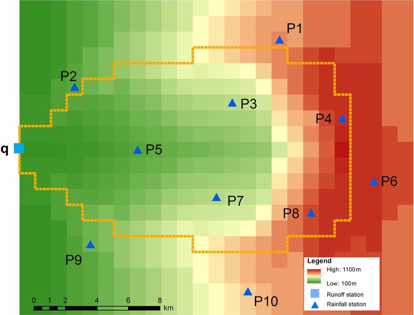
230 J. Grundmann et al.: Stochastic reconstruction of spatio-temporal rainfall patterns
ε (here, 1 − NSE is used). If a suitable solution is found the
whole procedure can be restarted using new random fields Vl .
Thus multiple solutions can be obtained enabling uncertainty
quantification of spatio-temporal rainfall fields.
3 Test of the methodology
3.1 Synthetic test site
To test the ability of the methodology a synthetic example
was designed. The example consists of a synthetic catch-
ment partly covered by rainfall. The synthetic catchment has
a size of 211 km2 with elevations ranging between 100 and
1100 m a.s.l. and homogeneous landscape properties (Fig. 2).
A synthetic rainfall event of 6 h duration with an hourly time
step and a maximum spatial extension of 118 km2 on a reg-
ular grid of 1 km by 1 km cell size is used. Rainfall amounts Figure 2. Topography, watershed, and observation network of the
above 20 mm event−1 cover an area of 25 km2 with maxi- synthetic catchment.
mum rainfall of 36 mm event−1 and maximum intensity of
12 mm h−1 (see Figs. 3 and S1 in the Supplement). Based
on this known spatio-temporal rainfall input pattern and RR
model parameterisation the catchment response at the sur-
face outlet was simulated and designated as the known “ob-
served” runoff qt (see Fig. 6, blue graph).
Furthermore, 10 different cells were selected from the
spatio-temporal rainfall patterns to represent virtual moni-
toring stations of rainfall. They were chosen in a way that
the centre of the event is not recorded. They are designated
as the known “observed” rainfall P xj , ti at J monitoring
stations for T time steps and provide the data basis for in-
terpolation, conditional simulation, and inverse modelling of
spatio-temporal rainfall patterns. Figure 4 shows their course
in time. Note that virtual monitoring stations 2, 5, 9, and 10
measure 0 mm h−1 rainfall only. Based on these observations
the fitted parameters for the marginal distribution (Eq. 3)
are p0 = 0.36 and λ = 0.48. The fitted copula for the depen- Figure 3. Rainfall amounts of the synthetic rainfall event. Virtual
dency structure in space and time is a Gaussian copula with monitoring stations are marked by crosses.
an exponential correlation function with a range of 2.5 km in
space and a range of 1.5 h in time. In comparison, using the
full synthetic dataset a range of 4.5 km in space and a range in Fig. 3. The maximum rainfall amount per event is equal to
of 2.5 h in time are estimated. the maximum of the observation at virtual station number 8
with 16.2 mm event−1 . Therefore, the extension of a rainfall
3.2 Results and discussion centre over 20 mm event−1 cannot be estimated. Due to low
rainfall intensities, the simulated response of the RR model
3.2.1 Common hydrologic modelling approach shows a significant underestimation of the observed runoff,
with an NSE value of −0.28 (see Fig. 6, green graph).
At first, hourly rainfall data from virtual monitoring stations
were used to interpolate the spatio-temporal rainfall patterns 3.2.2 Performance of conditional rainfall simulations
on a regular grid of 1 km by 1 km cell size by using the
inverse distance method, which is quite common in hydro- The Random Mixing approach was used to simulate 200 dif-
logic modelling. Afterwards, the response of the synthetic ferent spatio-temporal rainfall patterns conditioned on the
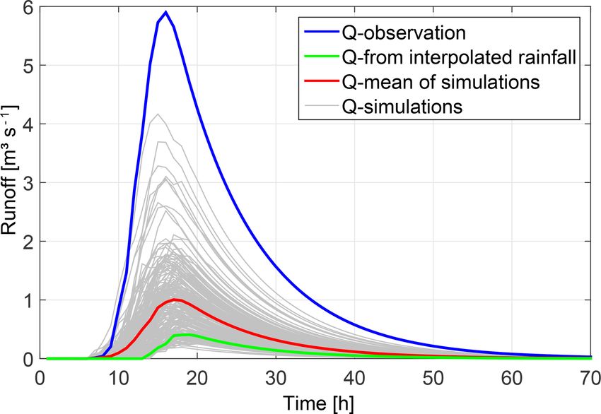
catchment was calculated by the RR model. Figure 5 shows virtual rainfall monitoring stations only. Resulting runoff
the interpolated pattern of the event-based rainfall amounts simulations are displayed in Fig. 6. They show a wide range
as the sum over single time steps. The pattern looks quite of hydrographs with peak values between 0.19 m2 s−1 and
smooth and has only minor similarities with the true pattern 4.17 m3 s−1 and NSE values between −0.37 and 0.89. Com-
Hydrol. Earth Syst. Sci., 23, 225–237, 2019 www.hydrol-earth-syst-sci.net/23/225/2019/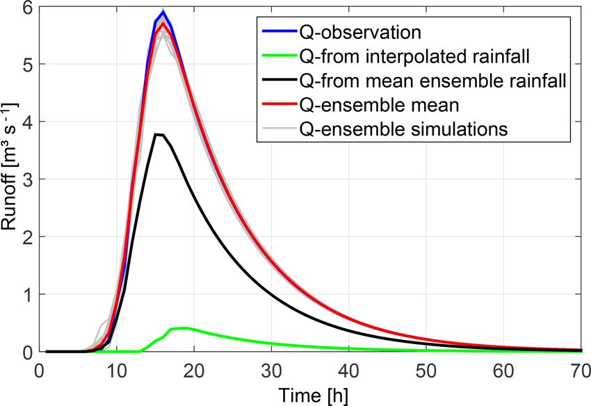
J. Grundmann et al.: Stochastic reconstruction of spatio-temporal rainfall patterns                                                     231

                                                                      Figure 6. Runoff simulations based on simulated spatio-temporal
                                                                      rainfall patterns conditioned at rainfall point observations only (grey
                                                                      graphs) compared to its mean (red graph), runoff observation (blue
Figure 4. Time series of rainfall intensities at virtual monitoring   graph), and simulation based on interpolated rainfall patterns (green
stations.                                                             graph).

                                                                      tual rainfall monitoring stations only are able to match the
                                                                      observed peak value in resulting runoff.

                                                                      3.2.3   Inverse hydrologic modelling approach

                                                                      The inverse modelling approach was used to simulate 107
                                                                      different spatio-temporal rainfall patterns which are con-
                                                                      ditioned on the virtual rainfall and runoff monitoring sta-
                                                                      tions, and runoff simulation results better than NSE values
                                                                      of 0.7. Afterwards a refinement was carried out by select-
                                                                      ing only those simulations with nearly identical runoff sim-
                                                                      ulation results compared to observations. These simulations
                                                                      are characterized by NSE values larger than 0.995. Figure 8
                                                                      shows the performance of the 20 selected realisations by grey
                                                                      graphs that show only minor deviations during the flood peak
                                                                      range compared to the observation (blue graph). Associated
Figure 5. Interpolated rainfall amounts per event by using data of    rainfall patterns are displayed in Fig. 9 for six selected re-
virtual monitoring stations.                                          alisations by their spatial rainfall amounts per event. Com-
                                                                      pared to the true spatial pattern (see Fig. 3) none of them
                                                                      reproduce the true pattern exactly, but all of them locate
pared to the runoff observation, the timing of peaks is accept-       the centre of the event in the same region as the true pat-
able, but the peak values are underestimated. Only four hy-           tern. This shows that by additional conditioning of spatio-
drographs have NSE values higher than 0.7. The correspond-            temporal rainfall patterns on runoff observation and consid-
ing spatial event-based rainfall amounts for the top three            eration of catchment’s drainage characteristic represented by
runoff simulations regarding the NSE values (a: 0.89, b: 0.78,        the RR model, the rainfall event can be localised and recon-
c: 0.73) is shown in Fig. 7. Their rainfall amounts range be-         structed in its spatial extent as well as in its course in time
tween 27.8 and 28.7 mm event−1 , with a spatial extent of 9           (see also Fig. S1). Most probably, if we would sample a large
to 11 km2 of rainfall above 20 mm event−1 and a maximum               number of rainfall fields conditioned on rainfall observation
intensity 10.5 to 15.1 mm h−1 . Compared to the observation           only, we would find a realisation which matches the runoff
(Fig. 3), the spatial patterns look similar, at least regarding       observation too. Due to additional conditioning on runoff we
the spatial location of the event, and cover the maximum in-          find these realisations faster.
tensity. But the rainfall amounts per event as well as their             However, the inference of a three-dimensional input vari-
spatial extent is too low. As a consequence, none of the sim-         able by using an integral output response results in a
ulated spatio-temporal rainfall fields conditioned at the vir-        set or ensemble of different solutions. Rainfall amounts

www.hydrol-earth-syst-sci.net/23/225/2019/                                             Hydrol. Earth Syst. Sci., 23, 225–237, 2019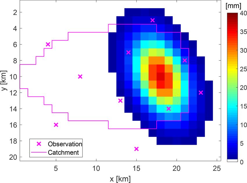
232                                        J. Grundmann et al.: Stochastic reconstruction of spatio-temporal rainfall patterns

Figure 7. Event-based rainfall patterns conditioned at rainfall point observations only for the top three runoff simulations in Fig. 6.

                                                                           the hydrograph simulation, since they are addressed by the
                                                                           initial and constant rate losses of the RR model.
                                                                              Deriving an average rainfall pattern by calculation of the
                                                                           mean value per grid cell over all realisations of the ensem-
                                                                           ble for each time step, a smoother pattern is obtained, which
                                                                           looks more similar to the true one but has smaller rainfall
                                                                           intensities. Using this mean ensemble pattern for calculat-
                                                                           ing the runoff response leads to an underestimation of the
                                                                           observed hydrograph as shown by the black hydrograph in
                                                                           Fig. 8. Therefore, the ensemble mean of the hydrographs (red
                                                                           line in Fig. 8) is a better representative for the sample than the
                                                                           mean ensemble rainfall pattern.
                                                                              In addition, data of the virtual monitoring stations (the ob-
                                                                           servation) have been always reproduced and are equal for
                                                                           each rainfall simulation. This means that each realisation re-
Figure 8. Comparison of hydrographs for the synthetic catchment            produces the point observation of rainfall without any un-
shown by the observed runoff (blue) and rainfall–runoff simulation         certainty. Only the grid points between the observation dif-
results based on interpolated rainfall patterns (green), a simulated       fer within the three-dimensional rainfall field and contain the
ensemble of spatio-temporal rainfall patterns conditioned at rainfall
                                                                           stochasticity given by rainfall simulations conditioned on the
and runoff observations (grey) and their mean value (red), and mean
ensemble rainfall patterns (black).
                                                                           observed values. In this context, the ensemble can be used as
                                                                           a partial descriptor of the total uncertainty. It describes the
                                                                           remaining uncertainty of precipitation if all available data
                                                                           are exploited under the assumption of error-free measure-
of the selected 20 realisations above 20 mm event−1 cover                  ments, reliable statistical rainfall models, and known hydro-
an area of 13 to 25 km2 with maximum rainfall of 26.7                      logic model parameters.
to 40.4 mm event−1 and maximum intensities of 10.7 to
17.1 mm h−1 . The event-based areal precipitation of the
catchment ranges between 98.2 % and 114.7 % of the obser-                  4     Application for real-world data
vation (see Fig. 3). Figure 9 presents spatial rainfall amounts
per event for (a) the realisation with the smallest area above             4.1    Arid catchment test site
20 mm event−1 and smallest intensity, (b) the realisation with
the largest area above 20 mm event−1 , (c) the realisation with            The real-world example is taken from the upper Wadi Bani
the highest intensity and rainfall amount per event, (d) the               Kharus in the northern part of the Sultanate of Oman. It is the
realisation with the best NSE value in resulting runoff, and               starting point for the present study and part of our multi-year
(e)–(f) realisations with similar event statistics like the true           research on hydrologic processes in this region. The head-
spatio-temporal rainfall pattern. Compared to the observed                 water under consideration is the catchment of the stream-
pattern (see Fig. 3), the different realisations match the spa-            flow gauging station of Al Awabi, with an area of 257 km2 ,
tial location as well as the shape of the observed pattern very            located in the Hadjar mountain range with heights ranging
well. However, the spatial patterns of the realisations are not            from 600 m a.s.l. to more than 2500 m a.s.l. The geology of
such smooth and symmetric like the constructed synthetic                   the area is dominated by the Hadjar group, which consists
observation. Furthermore, the realisations show some scat-                 of limestone and dolomite. The steep terrain consists mainly
tered low rainfall amounts, which are not of importance for                of rocks. Soils are negligible. However, larger units of al-

Hydrol. Earth Syst. Sci., 23, 225–237, 2019                                                www.hydrol-earth-syst-sci.net/23/225/2019/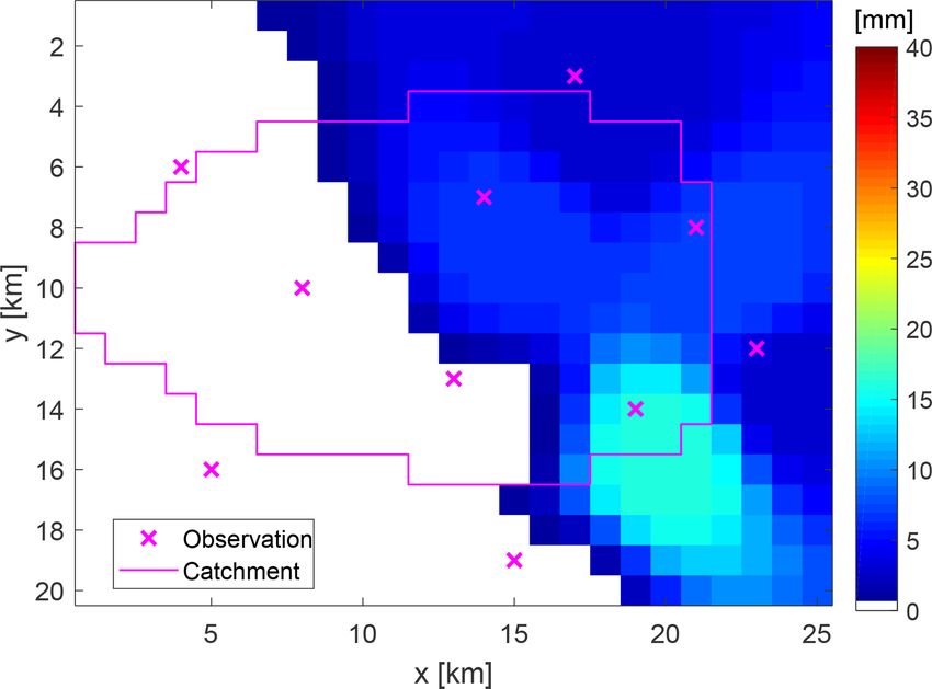
J. Grundmann et al.: Stochastic reconstruction of spatio-temporal rainfall patterns 233
Figure 9. Selected realisations of spatial rainfall amounts per event with similar performance in resulting runoff, obtained by the inverse
modelling approach for simulating spatio-temporal rainfall pattern: (a) realisation with the smallest area above 20 mm event−1 and smallest
intensity, (b) realisation with the largest area above 20 mm event−1 (c) realisation with the highest intensity and rainfall amount per event,
(d) realisation with the best NSE value in resulting runoff, and (e)–(f) realisations with similar event statistics to the true spatio-temporal
rainfall pattern.
luvial depositions in the valleys are important for hydro- 4.2 Results and discussion
logic processes, an issue which is addressed through spa-
tial differences in RR model parameters. Vegetation is sparse
and mostly cultivated in mountain oases. Annual rainfall can The real-world data example was performed for the runoff
reach more than 300 mm year−1 , showing a huge variabil- event from 12 February 1999 with an effective rainfall du-
ity between consecutive years. Analysis of measured runoff ration of 3 h. The simulated runoff for the interpolated rain-
data over a period of 24 years shows that runoff occurred fall pattern shows an underestimation of the peak discharge
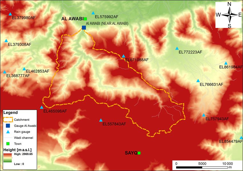
on average only on 18 days year−1 . Figure 10 displays the as well as a time shift of the peak arrival time compared to
available monitoring network for sub-daily data. Runoff is the observation (Fig. 12). Applying the inverse approach by
measured in 5 to 10 min temporal resolution. Rainfall mea- conditioning spatio-temporal rainfall patterns on rainfall and
surements vary from 1 min to 1 h. Therefore, a temporal res- runoff observations, an ensemble of 58 different hydrographs
olution of 1 h was chosen for the event under investigation in is obtained after refinement, with NSE values larger than 0.9.
this study. Figure 11 shows the measurements of the rainfall As shown in Fig. 12, all of these hydrographs (grey graphs)
gauging stations and their altitudes for the rainstorm from represent the observation well and overcome the time shift.
12 February 1999. Most of the rain was recorded on sta- To explain this behaviour, differential maps are calculated
tions with lower altitudes located in the north-west and south- which show the difference between the simulated and the in-
eastern part of the catchment. Rainfall interpolation was per- terpolated rainfall pattern for each time step (Fig. 13; see
formed by the inverse distance method, since there was no also Fig. S2 for comparison of event-based spatial rainfall
dependency of rainfall from altitude identifiable for this sin- amounts). It is easy to see that the inverse approach allows for
gle heavy rainfall event. Parameters for the inverse modelling a shift of the centre of the rainfall event from time step 1 to
approach are p0 = 0.17 and λ = 0.14 for the marginal distri- time step 2 and towards the catchment outlet. This results in
bution (Eq. 3). The fitted copula for the dependency structure a faster response of the catchment by its runoff compared to
in space and time is a Gaussian copula with an exponential the interpolated rainfall pattern. In general, the obtained en-
correlation function with a range of 10 km in space and a semble of spatio-temporal rainfall patterns is able to explain
range of 1 h in time. the observed runoff without discrepancy in rainfall measure-
ments. Similar to the synthetic example, the ensemble mean
hydrograph (Fig. 12, red graph) is a better representative for
www.hydrol-earth-syst-sci.net/23/225/2019/ Hydrol. Earth Syst. Sci., 23, 225–237, 2019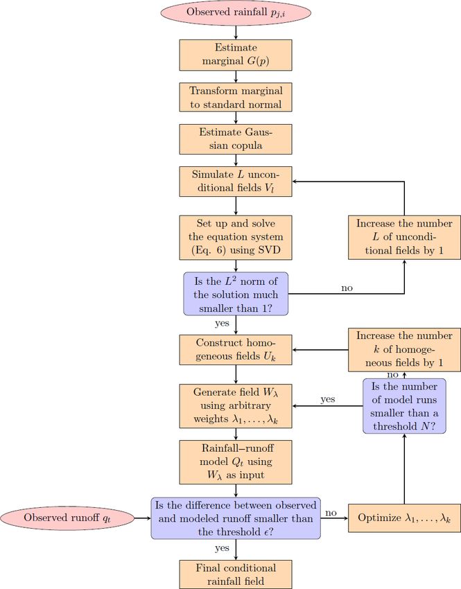
234                                      J. Grundmann et al.: Stochastic reconstruction of spatio-temporal rainfall patterns

Figure 10. Real-world case study: catchment of gauge Al Awabi and sub-daily monitoring network for runoff and rainfall.

                                                                      Figure 12. Comparison of hydrographs for the real-world catch-
                                                                      ment shown by the observed runoff (blue) and rainfall–runoff simu-
Figure 11. Rainfall amounts and altitudes of rainfall gauging sta-    lation results based on interpolated rainfall patterns (green), a sim-
tions from 12 February 1999.                                          ulated ensemble of spatio-temporal rainfall patterns conditioned at
                                                                      rainfall and runoff observations (grey) and their mean value (red),
                                                                      and mean ensemble rainfall patterns (black).
the sample than the hydrograph based on the mean ensemble
rainfall spatio-temporal pattern (black graph).
                                                                      reasonable spatio-temporal rainfall patterns conditioned on
                                                                      point rainfall and runoff observations. This has been demon-
5   Summary and conclusions                                           strated by a synthetic data example as well as a real-world
                                                                      data example for single rainstorms and catchments which are
An inverse hydrologic modelling approach for simulating               partly covered by rainfall.
spatio-temporal rainfall patterns is presented in this paper.            The proposed framework was compared to the methods of
The approach combines the conditional random field sim-               rainfall interpolation and conditional rainfall simulation. Re-
ulator Random Mixing and a spatial distributed RR model               construction of event-based spatio-temporal rainfall patterns
in a joint Monte Carlo framework. It allows for obtaining             has been feasible by the inverse approach, if runoff obser-

Hydrol. Earth Syst. Sci., 23, 225–237, 2019                                           www.hydrol-earth-syst-sci.net/23/225/2019/
J. Grundmann et al.: Stochastic reconstruction of spatio-temporal rainfall patterns 235 Figure 13. Differential maps of spatio-temporal rainfall patterns for three consecutive time steps (simulation – interpolation). vation and catchment’s spatial drainage characteristic repre- compared to an application of the whole ensemble due to sented by the RR model with spatial distributed travel times smoothing effects. of overland flow are considered. As shown by the synthetic The approach is also applicable under data-scarce situa- example, the rainfall pattern obtained by interpolation did not tions as demonstrated by a real-world data example. Here, match the observed rainfall field and runoff. If rain gauge ob- the flexibility of the approach becomes visible, since simu- servations do not portray the rain field adequately, a “good” lated rainfall patterns also allow for overcoming a shift in the interpolation result in the least-square sense is not a solu- timing of runoff. Therefore, the approach can be considered tion of the problem. This is the case in particular for small as a reanalysis tool for rainfall–runoff events, especially in scale rainstorms with high spatio-temporal rainfall variabil- regions where runoff generation and formation are based on ity and/or rainfall data scarcity due to insufficient monitor- surface flow processes (Hortonian runoff) and in catchments ing network density. By rainfall simulations conditioned on with wide ranges in arrival times at catchment outlets such rain gauge observation only, reasonable spatio-temporal rain- as mountainous regions or distinct drainage structures, e.g. fall fields are obtained, but with a wide spread in resulting urban and peri-urban regions. runoff hydrographs. A large number of simulated rainfall Nevertheless, further research and investigations are re- fields is required to find those realisations which match the quired. Examples presented in this paper are based on an observed runoff, since the amount of possible conditioned hourly time resolution and 1 km2 grid size in space. In par- rainfall fields is much higher than the amount of rainfall ticular, for rainstorms in small fast-responding catchments, fields matching point observation and runoff. By applying finer resolutions in space and time are required. Here the lim- optimisation, rainfall fields are conditioned on discharge too, its of the approach in the number of time steps and grid cells and appropriate candidates for spatio-temporal rainfall pat- need to be explored. Another point is the required amount terns can be identified more reliably, faster, and with reduced and quality of observation data as well as statistical model uncertainty. selection to obtain space–time rain fields. Both impact the The inference of a three-dimensional input variable by us- simulation of rainfall amounts and of patterns by the derived ing an integral output response results in a set of possible spatial and temporal dependence structure. In these exam- solutions in terms of spatio-temporal rainfall patterns. This ples Gaussian copulas are used, which might be not a good ensemble is obtained by repetitive execution of the optimi- estimator for the spatial dependency in any case of heavy sation step within the Monte Carlo loop. It can be consid- rainfall. ered as a descriptor of the partial uncertainty resulting from The proposed framework is a first step that only aims at spatio-temporal rainfall pattern estimates (under the assump- reconstructing spatio-temporal rainfall patterns under the as- tion of error-free measurements, reliable statistical rainfall sumption of fixed hydrologic model structure and param- models, and known hydrologic model parameters). Realisa- eters. Certainly, hydrologic model uncertainty is of impor- tions of the ensemble vary in rainfall amounts, intensities, tance. But instead of changing the model to fit the observed and spatial extent of the event, but they reproduce the point discharge, we estimate rainfall fields which fit the model and rainfall observation exactly and yield to similar runoff hydro- the discharge by doing reverse hydrology. As such plausi- graphs. This allows for deeper insights in hydrologic model ble rainfall fields can be identified, the corresponding model and catchment behaviour and gives valuable information for and the rainfall field is plausible. Thus, the framework can the reanalysis of rainfall–runoff events, since rainstorm con- be applied to proof hypothesis about hydrologic model se- figurations leading to similar flood responses become visi- lection or to explain extraordinary rainfall–runoff events by ble. As shown in the example, operating with an ensemble using a well calibrated, spatial distributed hydrologic model mean is less successful in matching the runoff observation for the catchment of interest. In this context, further research www.hydrol-earth-syst-sci.net/23/225/2019/ Hydrol. Earth Syst. Sci., 23, 225–237, 2019
236                                       J. Grundmann et al.: Stochastic reconstruction of spatio-temporal rainfall patterns

is dedicated to providing a common interface within the                 Bárdossy, A.: Interpolation of groundwater quality parameters with
Monte Carlo framework to exchange the hydrologic model                    some values below the detection limit, Hydrol. Earth Syst.
and allow for broader use within the community. Also, fur-                Sci., 15, 2763–2775, https://doi.org/10.5194/hess-15-2763-2011,
ther sources of uncertainties (e.g. model parameters, obser-              2011.
vations) need to be considered to contribute for the solution           Bárdossy, A. and Hörning, S.: Random Mixing: An Ap-
                                                                          proach to Inverse Modeling for Groundwater Flow and
of the hydrologic modelling uncertainty puzzle.
                                                                          Transport Problems, Transport Porous Med., 114, 241–259,
                                                                          https://doi.org/10.1007/s11242-015-0608-4, 2016a.
                                                                        Bárdossy, A. and Hörning, S.: Gaussian and non-Gaussian
Data availability. All data (except for confidential data) can be re-     inverse modeling of groundwater flow using copulas
quested via email (jens.grundmann@tu-dresden.de).                         and random mixing, Water Resour. Res., 52, 4504–4526,
                                                                          https://doi.org/10.1002/2014WR016820, 2016b.
                                                                        Bell, T. L.: A space-time stochastic model of rainfall for satel-
Supplement. The supplement related to this article is available           lite remote-sensing studies, J. Geophys. Res.-Atmos., 92, 9631–
online at: https://doi.org/10.5194/hess-23-225-2019-supplement.           9643, https://doi.org/10.1029/JD092iD08p09631, 1987.
                                                                        Beven, K. and Hornberger, G.: Assessing the effect of spatial pat-
                                                                          tern of precipitation in modeling stream-flow hydrographs, Water
Author contributions. JG and AB conceived and designed the                Resour. Bull., 18, 823–829, 1982.
study. JG and SH performed the analysis and wrote the paper. AB         Casper, M. C., Herbst, M., Grundmann, J., Buchholz, O., and
contributed to the interpretation of the results and commented on         Bliefernicht, J.: Influence of rainfall variability on the simulation
the paper.                                                                of extreme runoff in small catchments, Hydrol. Wasserbewirts.,
                                                                          53, 134–139, 2009.
                                                                        Chaubey, I., Haan, C., Grunwald, S., and Salisbury, J.: Uncer-
Competing interests. The authors declare that they have no conflict       tainty in the model parameters due to spatial variability of
of interest.                                                              rainfall, J. Hydrol., 220, 48–61, https://doi.org/10.1016/S0022-
                                                                          1694(99)00063-3, 1999.
                                                                        Del Giudice, D., Albert, C., Rieckermann, J., and Reichert, P.: De-
Acknowledgements. The corresponding author wishes to thank                scribing the catchment-averaged precipitation as a stochastic pro-
the Ministry of Regional Municipalities and Water Resources of            cess improves parameter and input estimation, Water Resour.
the Sultanate of Oman for providing the data for the real case            Res., 52, 3162–3186, https://doi.org/10.1002/2015WR017871,
study and supporting the joint Omani–German IWRM-APPM                     2016.
initiative. Research for this paper was partly supported by the         Dyck, S. and Peschke, G.: Grundlagen der Hydrologie, Verlag für
German Research Foundation (Deutsche Forschungsgemeinschaft,              Bauwesen Berlin, 1983.
no. 403207337, BA 1150/24-1) and partly by the Energi Simulation        Faures, J., Goodrich, D., Woolhiser, D., and Sorooshian, S.: Im-
Program. Furthermore, we acknowledge support by the Open                  pact of small-scale spatial rainfall variability on runoff mod-
Access Publication Funds of the SLUB/TU Dresden.                          eling, J. Hydrol., 173, 309–326, https://doi.org/10.1016/0022-
                                                                          1694(95)02704-S, 1995.
Edited by: Nadav Peleg                                                  Gerner, A.: A novel strategy for estimating groundwater recharge
Reviewed by: two anonymous referees                                       in arid mountain regions and its application to parts of the Jebel
                                                                          Akhdar Mountains (Sultanate of Oman), PhD thesis, Technische
                                                                          Universität Dresden, 2013.
                                                                        Golub, G. and Kahan, W.: Calculating the Singular Values and
                                                                          Pseudo-Inverse of a Matrix, J. Soc. Ind. Appl. Math., 2, 205–224,
References                                                                1965.
                                                                        Gunkel, A. and Lange, J.: New Insights Into The Natural Variabil-
Al-Qurashi, A., McIntyre, N., Wheater, H., and Unkrich,                   ity of Water Resources in The Lower Jordan River Basin, Water
  C.: Application of the Kineros2 rainfall-runoff model to                Resour. Manage., 26, 963–980, https://doi.org/10.1007/s11269-
  an arid catchment in Oman, J. Hydrol., 355, 91–105,                     011-9903-1, 2012.
  https://doi.org/10.1016/j.jhydrol.2008.03.022, 2008.                  Haese, B., Horning, S., Chwala, C., Bardossy, A., Schalge, B., and
Andreassian, V., Perrin, C., Michel, C., Usart-Sanchez, I., and           Kunstmann, H.: Stochastic Reconstruction and Interpolation of
  Lavabre, J.: Impact of imperfect rainfall knowledge on the ef-          Precipitation Fields Using Combined Information of Commer-
  ficiency and the parameters of watershed models, J. Hydrol.,            cial Microwave Links and Rain Gauges, Water Resour. Res., 53,
  250, 206–223, https://doi.org/10.1016/S0022-1694(01)00437-1,            10740–10756, 2017.
  2001.                                                                 Hörning, S.: Process-oriented modeling of spatial random fields us-
Bahat, Y., Grodek, T., Lekach, J., and Morin, E.: Rainfall-runoff         ing copulas, Eigenverlag des Instituts für Wasser- und Umwelt-
  modeling in a small hyper-arid catchment, J. Hydrol., 373, 204–         systemmodellierung der Universität Stuttgart, 2016.
  217, https://doi.org/10.1016/j.jhydrol.2009.04.026, 2009.             Hu, L.: Gradual deformation and iterative calibration of Gaussian-
Bárdossy, A.: Copula-based geostatistical models for ground-              related stochastic models, Math Geol., 32, 87–108, 2000.
  water quality parameters, Water Resour. Res., 42, W11416,
  https://doi.org/10.1029/2005WR004754, 2006.

Hydrol. Earth Syst. Sci., 23, 225–237, 2019                                              www.hydrol-earth-syst-sci.net/23/225/2019/
J. Grundmann et al.: Stochastic reconstruction of spatio-temporal rainfall patterns 237 Journel, A.: Geostatistics for conditional simulation of ore bodies, Obled, C., Wendling, J., and Beven, K.: The sensitivity of Econ. Geol., 69, 673–687, 1974. hydrological models to spatial rainfall patterns – an eval- Kavetski, D., Kuczera, G., and Franks, S.: Bayesian uation using observed data, J. Hydrol., 159, 305–333, analysis of input uncertainty in hydrological mod- https://doi.org/10.1016/0022-1694(94)90263-1, 1994. eling: 1. Theory, Water Resour. Res., 42, W03407, Paschalis, A., Molnar, P., Fatichi, S., and Burlando, P.: https://doi.org/10.1029/2005WR004368, 2006. A stochastic model for high-resolution space-time precip- Kirchner, J. W.: Catchments as simple dynamical systems: itation simulation, Water Resour. Res., 49, 8400–8417, Catchment characterization, rainfall-runoff modeling, and do- https://doi.org/10.1002/2013WR014437, 2013. ing hydrology backward, Water Resour. Res., 45, W02429, Paschalis, A., Fatichi, S., Molnar, P., Rimkus, S., and Burlando, https://doi.org/10.1029/2008WR006912, 2009. P.: On the effects of small scale space-time variability of Krajewski, W. F., Lakshmi, V., Georgakakos, K. P., and Jain, S. C.: rainfall on basin flood response, J. Hydrol., 514, 313–327, A Monte Carlo Study of rainfall sampling effect on a dis- https://doi.org/10.1016/j.jhydrol.2014.04.014, 2014. tributed catchment model, Water Resour. Res., 27, 119–128, Pegram, G. and Clothier, A.: High resolution space-time modelling https://doi.org/10.1029/90WR01977, 1991. of rainfall: the “String of Beads” model, J. Hydrol., 241, 26–41, Kretzschmar, A., Tych, W., and Chappell, N. A.: Revers- https://doi.org/10.1016/S0022-1694(00)00373-5, 2001. ing hydrology: Estimation of sub-hourly rainfall time-series Peleg, N., Fatichi, S., Paschalis, A., Molnar, P., and Burlando, P.: An from streamflow, Environ. Modell. Softw., 60, 290–301, advanced stochastic weather generator for simulating 2-D high- https://doi.org/10.1016/j.envsoft.2014.06.017, 2014. resolution climate variables, J. Adv. Model. Earth Sy., 9, 1595– Leblois, E. and Creutin, J.-D.: Space-time simulation of inter- 1627, https://doi.org/10.1002/2016MS000854, 2017. mittent rainfall with prescribed advection field: Adaptation of Pilgrim, D., Chapman, T., and Doran, D.: Problems of rainfall- the turning band method, Water Resour. Res., 49, 3375–3387, runoff modeling in arid and semiarid regions, Hydrolog. Sci. https://doi.org/10.1002/wrcr.20190, 2013. J., 33, 379–400, https://doi.org/10.1080/02626668809491261, Le Ravalec, M., Noetinger, B., and Hu, L. Y.: The FFT Moving 1988. Average (FFT-MA) Generator: An Efficient Numerical Method Renard, B., Kavetski, D., Leblois, E., Thyer, M., Kuczera, G., and for Generating and Conditioning Gaussian Simulations, Math. Franks, S. W.: Toward a reliable decomposition of predictive un- Geol., 32, 701–723, 2000. certainty in hydrological modeling: Characterizing rainfall errors Li, J.: Application of Copulas as a New Geostatistical Tool, Eigen- using conditional simulation, Water Resour. Res., 47, W11516, verlag des Instituts für Wasser- und Umweltsystemmodellierung https://doi.org/10.1029/2011WR010643, 2011. der Universität Stuttgart, 2010. Shah, S., O’Connell, P., and Hosking, J.: Modelling the effects of Lopes, V.: On the effect of uncertainty in spatial distribution spatial variability in rainfall on catchment response. 2. Experi- of rainfall on catchment modelling, Catena, 28, 107–119, ments with distributed and lumped models, J. Hydrol., 175, 89– https://doi.org/10.1016/S0341-8162(96)00030-6, 1996. 111, https://doi.org/10.1016/S0022-1694(96)80007-2, 1996. Mantoglou, A. and Wilson, J.: The Turning Bands Method Shinozuka, M. and Deodatis, G.: Simulation of stochastic pro- for simulation of random fields using line generation by cesses by spectral representation, Appl. Mech. Rev., 44, 191– a spectral method, Water Resour. Res., 18, 1379–1394, 204, https://doi.org/10.1115/1.3119501, 1991. https://doi.org/10.1029/WR018i005p01379, 1982. Shinozuka, M. and Deodatis, G.: Simulation of multi-dimensional McIntyre, N., Al-Qurashi, A., and Wheater, H.: Regression Gaussian stochastic fields by spectral representation, Appl. analysis of rainfall-runoff data from an arid catchment in Mech. Rev., 49, 29–53, https://doi.org/10.1115/1.3101883, 1996. Oman, Hydrolog. Sci. J., 52, 1103–1118, International Con- Troutman, B.: Runoff prediction errors and bias in ference on Future of Drylands, Tunis, Tunisia, June 2006, parameter-estimation induced by spatial variability https://doi.org/10.1623/hysj.52.6.1103, 2007. of precipitation, Water Resour. Res., 19, 791–810, McMillan, H., Jackson, B., Clark, M., Kavetski, D., and Woods, https://doi.org/10.1029/WR019i003p00791, 1983. R.: Rainfall uncertainty in hydrological modelling: An evalu- Wilks, D.: Multisite generalization of a daily stochastic pre- ation of multiplicative error models, J. Hydrol., 400, 83–94, cipitation generation model, J. Hydrol., 210, 178–191, https://doi.org/10.1016/j.jhydrol.2011.01.026, 2011. https://doi.org/10.1016/S0022-1694(98)00186-3, 1998. Morin, E., Goodrich, D., Maddox, R., Gao, X., Gupta, H., Wood, A.: When is a truncated covariance function on the line a and Sorooshian, S.: Spatial patterns in thunderstorm covariance function on the circle?, Stat. Probabil. Lett., 24, 157– rainfall events and their coupling with watershed hy- 164, 1995. drological response, Adv. Water Resour., 29, 843–860, Wood, A. and Chan, G.: Simulation of stationary Gaussian process https://doi.org/10.1016/j.advwatres.2005.07.014, 2006. in [0, 1]d , J. Comput. Graph. Stat., 3, 409–432, 1994. Nash, J. and Sutcliffe, J.: River flow forecasting through conceptual models part I – A discussion of principles, J. Hydrol., 10, 282– 290, https://doi.org/10.1016/0022-1694(70)90255-6, 1970. Nicotina, L., Celegon, E. A., Rinaldo, A., and Marani, M.: On the impact of rainfall patterns on the hy- drologic response, Water Resour. Res., 44, W12401, https://doi.org/10.1029/2007WR006654, 2008. www.hydrol-earth-syst-sci.net/23/225/2019/ Hydrol. Earth Syst. Sci., 23, 225–237, 2019
You can also read