Grid-Based Anomaly Detection of Freight Vehicle Trajectory considering Local Temporal Window

Hindawi
Journal of Advanced Transportation
Volume 2021, Article ID 8103333, 18 pages
https://doi.org/10.1155/2021/8103333

Research Article
Grid-Based Anomaly Detection of Freight Vehicle
Trajectory considering Local Temporal Window

 Zixian Zhang,1,2 Geqi Qi ,1,2,3 Avishai (Avi) Ceder,1,4 Wei Guan ,1,2 Rongge Guo,1,2
 and Zhenlin Wei1,2
 1
 Key Laboratory of Transport Industry of Big Data Application Technologies for Comprehensive Transport, Ministry of Transport,
 Beijing Jiaotong University, Beijing 100044, China
 2
 School of Traffic and Transportation, Beijing Jiaotong University, Beijing 100044, China
 3
 Beijing Research Center of Urban Traffic Information Sensing and Service Technologies, Beijing Jiaotong University,
 Beijing 100044, China
 4
 Faculty of Civil and Environmental Engineering and the Transportation Research Institute,
 Technion-Israel Institute of Technology, Technion City, Haifa 32000, Israel

 Correspondence should be addressed to Wei Guan; weig@bjtu.edu.cn

 Received 18 April 2021; Revised 23 July 2021; Accepted 12 August 2021; Published 31 August 2021

 Academic Editor: Dung-Ying Lin

 Copyright © 2021 Zixian Zhang et al. This is an open access article distributed under the Creative Commons Attribution License,
 which permits unrestricted use, distribution, and reproduction in any medium, provided the original work is properly cited.
 The security travel of freight vehicles is of high societal concern and is the key issue for urban managers to effectively supervise and
 assess the possible social security risks. With continuous improvements in motion-based technology, the trajectories of freight
 vehicles are readily available, whose unusual changes may indicate hidden urban risks. Moreover, the increasing high spatial and
 temporal resolution of trajectories provides the opportunity for the real-time recognition of the abnormal or risky vehicle motion.
 However, the existing researches mainly focus on the spatial anomaly detection, and there are few researches on the real-time
 temporal anomaly detection. In this paper, a grid-based algorithm, which combines the spatial and temporal anomaly detection, is
 proposed for tracing the risk of urban freight vehicles trajectory by considering local temporal window. The travel time probability
 distribution of vehicle historical trajectory is analyzed to meet the time complexity requirements of real-time anomaly calculation.
 The developed methodology is applied to a case study in Beijing to demonstrate its accuracy and effectiveness.

1. Introduction The unusual change of real-time trajectory may indicate
 the potential risk in spatial and temporal dimensions.
With respect to urban security, logistics trajectories security Anomaly trajectory detection aims to find a trajectory that is
plays an important role, which deserves a closer look. In significantly different from most of the historical trajectories
particular, during major events such as the ceremony, with the same origin and destination. It is mainly reflected in
concert, and games, real-time monitoring and anomaly the process of freight vehicles driving from the station to the
detection of the logistics vehicles trajectories have attracted a distribution point. Due to the behavior habits of drivers and
large amount of security concern since the tragedy in Nice the periodicity of urban traffic, freight vehicles have similar
(86 dead and 458 injured) [1] and Barcelona (15 dead and driving paths with the same starting and ending points at the
100 injured). As the vehicle trajectory data can be conve- same time. In the field of anomaly detection of trajectory,
niently collected nowadays by digital sensors, such as various many studies have been investigated from different per-
navigation systems, smart cellphones, and RFID devices, spectives [11–13], some of which are used to detect deceptive
researchers can study the reliability of trajectories and the driving behavior in taxi drivers. However, these studies
invoked transportation risk issues, i.e., driving behavior mainly focus on the spatial anomaly detection, and there are
detection [2, 3], travel pattern recognition [4–6], and few related to the temporal anomaly detection. In terms of
anomaly tracking in practice [4–10]. existing research methods, the research on space abnormal

2 Journal of Advanced Transportation

trajectory detection can be segmented into three main results of three trajectory datasets are analyzed using the
categories. The first category is based on distance and density algorithm proposed in this paper. In Section 5, the per-
[14, 15]. This category of method usually requires calculating formance of the algorithm is analyzed. In Section 6, the the
metrics based on the entire historical database, which leads adjustment mechanism of the algorithm is discussed. In
to high time complexity. The second category is based on Section 7, we summarize and discuss the whole paper.
architecture, mainly neural network architecture and rein-
forcement learning architecture [16, 17]. This type of method 2. Related Research
requires a large number of tags, and its accuracy is directly
related to the quality of the data. The third category is pattern The trajectory data have been widely used in the popular
based [11, 13]. This type of method mainly studies the route discovery and anomaly detection. In the field of
cooccurrence of trajectory points, so that abnormal trajec- popular route discovery, Zaiben et al. [18] proposed a co-
tories with low probabilities can be detected in a preset herence expanding algorithm and a maximum probability
window. product algorithm to discover the most popular route. Jani
 However, there are few related researches on real-time et al. [19] used a fast map server, which could generate and
temporal anomaly discovery, which can help find the ab- visualize hot maps of hot routes online from massive motion
normal location of vehicles from the temporal perspective. trajectory data according to customers’ preferences. Luo
This may be due to the following reasons: (1) urban et al. [20] found that suffix-optimal, length-insensitive, and
transportation network flow is dynamic and complex, which bottleneck-free methods reflect common-sense notions and
leads to the different temporal security assessment threshold proposed efficient search algorithms to determine the most
corresponding to different spatial locations, such that in- frequently used paths based on the time period. The se-
tersection parking and road section parking are different; (2) mantic features mainly come from other moving objects
spatial anomaly can be judged by the isolated trajectory with similar behaviors. Treerapot et al. [21] proposed a
point, while temporal anomaly detection required a detec- statistical approach to estimate truck activities and freight
tion window cooperating multiple sequential trajectory analytics from Global Positioning System (GPS) data of
point; (3) in real-time detection, selecting an appropriate trucks and applied the method in estimating activities, ac-
detection window size is critical, and unreasonable selection tivity patterns, commodity trip chains, and status of trips
may lead to completely wrong judgment. In extreme ex- legs from the collected truck GPS data. Wei et al. [22] studied
ample, with only one trajectory point in the window, the the characteristics of uncertain trajectories and proposed a
travel time anomaly of a single trajectory point may be slight. route inference framework based on a collective knowledge
However, with the expansion of time window, it is possible algorithm to find the top-k popular routes. Outlier detection
to exceed the threshold set by the detection window of is important work in mining trajectories [23, 24]. Lee and
historical trajectories. Cho et al. [24] proposed a grid-based local outlier factor
 In light of this, the window time of isolation based online algorithm for outlier detection. This algorithm reduces the
anomalous trajectory detection (WT-iBOAT) algorithm is computation time significantly with acceptable trade-off
proposed in this paper to accomplish the real-time anomaly errors. Knorr et al. [23] studied the notion of distance-based
detection of abnormal logistics trajectories. The research can outliers to find outliers in multidimensional datasets. Dis-
help supervise the driver of logistics vehicles to drive the covering the popular route is always used for daily man-
vehicle safely and reliably and enable the real-time anomaly agement and operation of urban traffics. Sometimes, it is
detection of freight vehicle trajectories by considering both helpful to find out the abnormal trajectories, but it lacks
spatial and temporal variations. The main contributions are directness compared with anomaly detection and may result
as follows: in misidentification of some regular trajectories (not most
 popular ones).
 (i) First, we extract different constraints from not only In the field of anomaly detection, Wang et al. [25] uesd
 spatial, but also temporal dimensions for compre- improved Robust Rrincipal Component Analysis (RPCA) to
 hensively solving the motion-based anomaly de- introduce the detection of abnormal passenger flow and
 tection problem Spatial Temporal-Density-Based Spatial Clustering of Ap-
 (ii) Second, a grid-based anomaly detection method is plication with Noise (ST-DBSCAN) algorithm to group the
 proposed from a new perspective of using the local detected station-level anomalies. Suzuki et al. [26] applied
 temporal window, which is beneficial for increasing the hidden Markov model (HMM) and k-means, and Bera
 calculation accuracy and reducing the computation et al. [7] used Bayesian learning techniques to detect ab-
 complexity of real-time detection normal pedestrian trajectories. Other popular fields related
 to GPS traces include the detection of social communities
 (iii) Third, this paper proposes a framework for
 [27] and abnormal driver behavior [28]. Yin et al. [27]
 detecting real-time risk trajectories of urban freight
 proposed a probabilistic model, which was used to infer
 vehicles, and a real-world data set is utilized to verify
 users’ social communities by integrating their spatiotem-
 its feasibility
 poral data and semantic information. Ali and Ismail [28]
 The paper is organized as follows. In Section 2, the investigated driver behavior through GPS trajectory data
relevant work is investigated. In Section 3, related archi- from the vehicle, mainly considering the features of speed
tectures and algorithms are proposed. In Section 4, the limit, sudden speed changes, and constant changes in the

Journal of Advanced Transportation 3

vehicle lateral position, and they used these features to detect new abnormalities. Yingyi et al. [31] proposed a method of
abnormal driver behavior. monitoring distance-based anomalies over trajectory
 Many researchers have conducted related research on streams. This method mainly used local clustering and
abnormal trajectory detection. In Song et al. [16], in order to piecewise vantage point trees with the corresponding
solve the problems, i.e., the traditional anomaly trajectory pruning method to reduce the calculation time. These
detection method cannot adequately capture the sequence studies can make efficient detecting trajectory outlier while
information of the trajectory, and focusing only on the given preserving the effectiveness. But these algorithms only study
source and target may lead to data sparseness. They proposed space anomaly detection and do not relate the temporal
an algorithm that used an Anomalous Trajectory Detection anomaly detection.
using Recurrent Neural Network (ATD-RNN) to represent the Jie et al. [12] used a historical trajectory dataset and
trajectory by learning a trajectory embedding and then found commonly detected abnormal trajectories. Then, they
the risk trajectory. Liping et al. [15] put forward a trajectory modified the TPRO algorithm by dividing the steps into
segmentation strategy based on multimotion features and a offline processing and online detection and adding appro-
similarity measurement method based on trajectory structures. priate modules to adapt the detection. This paper proposed
With the proposed strategy and method, a distributed tra- an algorithm named trajectory outlier detection (TPRRO).
jectory clustering algorithm is designed to improve the effi- TPRRO is a real-time outlier detection algorithm, and it
ciency of the clustering algorithm. To tackle the problem of constructs short for time-dependent transfer index (TTI)
calculating distance and neighborhood density in the trajectory and short for time-dependent transfer graph (TTG) to
anomaly detection algorithm, the dataset was pruned by the conduct spatiotemporal anomaly detection. Although this
trajectory clustering results, which improves the efficiency of paper proposed an algorithm for temporal anomaly detec-
the algorithm. Nonetheless, Song et al. [16] and Liping et al. tion, it did not analyze temporal anomaly detection in detail.
[15] required artificial label of abnormal trajectory for im- At the same time, Jie et al. [12] used time-dependent transfer
proving effective of algorithm and could not perform real-time graph (TTG), which calculated the travel time from a vertex
anomaly detection. to another in road network, so this algorithm could not
 Wu et al. [17] proposed a probabilistic model-based reflect immediate temporal anomaly information of
vehicle outlier detection method, Driving Behavior-based trajectory.
Trajectory Outlier Detection (DB-TOD), which was used to In summary, we present a real-time temporal anomaly
model the driving behavior in a historical trajectory set. They detection algorithm for logistic vehicle to prevent potential
designed outlier detection algorithms for both full and security incidents. Different from the previous study (in
partial outliers, which solved the problem for providing early Table 1, we summarize contributions of previous study and
warnings of outliers only when the outliers were partially our research), we focus on the real-time temporal anomaly
observed. Lee et al. [8] et al. aimed to address the problem detection method and design algorithmic framework for
that the detection algorithm for tracking outliers has limited spatiotemporal anomaly detection of Urban Freight Vehi-
ability in detecting the outliers’ tracks. An outlier detection cles. We further conduct analysis to our collecting data and
algorithm, time-dependent popular route-based trajectory explain the possible motivations and reasons of the
outlier detection (TPRO), was proposed. The algorithm was anomalous behaviors.
divided into two stages: partitioning and detection. For the
first stage, a two-layer trajectory partition strategy has en- 3. Methods
sured the high quality and high efficiency of subtrajectory
partitioning. In the second stage, the hybrid outlier detection In this section, the algorithmic framework of this paper is
method based on distance and density clustering improves introduced, including data preprocessing (DP), offline
the accuracy of the trajectory outlier detection algorithm. processing (OFP), the data manager (DM), and online
Daqing et al. [11] proposed an isolation-based anomalous processing (OLP). The purpose of DP is to obtain the ef-
trajectory (iBAT) method based on isolation. First, the fective loading and unloading positions of raw GPS data. The
original trajectory was mapped into the grid sequence, and goal of OFP is to obtain the available subtrajectories from the
the historical grid trajectory index was established. Then, the loading (origin) and unloading (destination) positions ob-
iForest algorithm was used to detect the isolated trajectory. tained from the DP and to mapping the subtrajectories to a
However, this approach can only support full trajectories. preset grid. The goal of OLP is to real-timely meshing test
Sun et al. [29] proposed the iBOAT algorithm based on trajectory points. The DM is mainly used for extraction of
trajectories, similar to the real-time detection method, which spatiotemporal experience constrained from the historical
was an influential method. This method was developed from trajectories and detect abnormal trajectories. Figure 1 shows
the iBAT algorithm. The main improvement of this method the submodules within the modules.
is the way that it compares with iBAT in view of the whole
line offline, as it is improved by using the method of real-
time contrast. It is more practical, because it can be a fast 3.1. Concept Relationship. This section first introduces the
detection algorithm with high reliability. Yu et al. [30] relationship among the concepts involved. For trajectory
defined anomalous behavior of moving objects according to anomaly detection, the relationship between trajectory point
the idea of neighbor-based trajectory outliers and proposed and time/loading position/unloading positions is many-to-
the minimal examination framework to effectively discover one, because many trajectory points are associated with the

4 Journal of Advanced Transportation

 Table 1: Comparison between previous works and the work presented.
 Characteristics of works related to efficient feeder/shuttle bus services
 Paper Results Results of
No. Spatio Temporal Every
 (chronologically) anomaly Between road of spatio temporal
 anomaly Real-time trajectory Based-gird Based-graph
 intersections anomaly anomaly
 detection detection point
 detection detection
1 Yingyi Bu et al. ✓ ✓
 Daqing Zhang
2 ✓ ✓ ✓ ✓
 et al.
 LingYin Wei
3 ✓ ✓ ✓ ✓
 et al.
4 Sun L et al. ✓ ✓ ✓ ✓ ✓
 Wuman Luo
5 ✓ ✓
 et al.
6 Yu Y et al. ✓ ✓
7 Jie Zhu et al. ✓ ✓ ✓ ✓ ✓
8 Liping Lu et al. ✓ ✓ ✓
9 Wu H et al. ✓ ✓ ✓
10 Li Song et al. ✓ ✓ ✓
 Treerapot
11 ✓ ✓ ✓
 Siripirote et al.
 Zhang et al. (this
12 ✓ ✓ ✓ ✓ ✓ ✓ ✓
 paper)

same time/loading position/unloading position. For the COLN max − COLN min
same loading and unloading positions, the trajectories are X� ,
 k
different in different time periods. A loading position may be (1)
related to the trajectory of different roads, different times, ROWN max − ROWN min
 Y� .
and different unloading positions. In addition, trajectories k
crossing a specific road section may involve different loading
positions; trajectories crossing a specific road section and
different unloading positions may also involve similar 3.3. Rough Selection of the Trajectory Set. Before anomaly
relationships. detection of test trajectory, we first need to filter the historical
 trajectory, which has the same loading and unloading point as
3.2. Meshing of the Spatiotemporal Trajectory Point. The the test trajectory. We define this process as the query of
movement of vehicles produces a lot of trajectory data. We historical trajectory. The related concepts are defined as follows:
need to divide the existing historical trajectory effectively
before detecting the spatiotemporal anomaly of trajectory. Definition 1 (trajectory). Trajectories tr � {P1, P2, ..., PN} are
The granularity of spatiotemporal trajectories is crucial when collected GPS records. Each GPS record Pi specifies the
dividing trajectories. Different mesh sizes are suitable for instantaneous time, position (latitude and longitude), and
different trajectory granularity problems. This is the reason vehicle ID of the vehicle.
why we use the grid method, which does not require us to
know all the space-time coordinates, which avoid a lot of Definition 2 (subtrajectory). The subtrajectory reflects dif-
calculation. The trajectory point is mapped to the two-di- ferent driving preferences of different drivers for vehicles
mensional space of the grid cell (Figure 2). This is a two- with the same transportation purpose in different periods.
dimensional Euclidean space defined by x-axis and y-axis. The We use the effective parking time as the division factor of the
center of each grid cell is used to represent all GPS points of subtrajectory. So, the subtrajectory is a part of the trajectory.
the grid cell. If the grid cell is too large, the accuracy of
anomaly detection may not be enough. However, the smaller Definition 3 (scalable loading and unloading point of tra-
grid cell may lead to much computation. Therefore, we must jectories). In order to eliminate irrelevant trajectories, the
find an optimal grid size that can identify trajectories without loading and unloading points are used as spatial constraints
unnecessary computation. Based on two-dimensional grid to filter all trajectories. In order to achieve this goal, we first
division, the trajectory query from specific loading position find loading points for all the subtrajectories and keep the
coordinates to specific unloading position coordinates be- subtrajectories. After that, we find the corresponding
comes the trajectory query from one grid cell to another. unloading point in kept subtrajectories. Compared with the
 We define the minimum range of grid as (COLNmin, common input method, this method has a huge advantage: a
ROWNmin, COLNmax, ROWNmax) and the length range trajectory is used in anomaly detection when the middle
of a grid as k. X and Y present the numbers of columns and section of this trajectory has the same loading and unloading
rows of grid in the study area [32]. points as the test trajectory, as shown in Figure 2.

Journal of Advanced Transportation 5

 Analysis of
 OD
 Task analysis vehicle
 clustering
 parking time

 Data pre–
 processing

 0 D D
 0
 Trajectory

 0 D 0 D
 Offline Sub–
 processing trajectory

 Meshing

 Real-time
 Data manager abnormal
 trajectory
 Rough selection of the Extraction of Spatiotemporal detection
 trajectory set Constrained experience

 Real-time
 Meshing

 Online
 processing 0 D Scalable
 OD

 Test
 trajectory

 Figure 1: Algorithm framework.

3.4. Extraction of Spatiotemporal Constraint are as follows. Suppose that there are three purple trajec-
 tories in Figure 3, T � , where t1 � , t2 � ,
period; this difference comes from drivers’ perception of t3 � , and a test trajectory t � , then hasPath (T, t) � {t2, t3}. So, hasPath is
optional travel in a fixed time is regular and searchable. defined as a function that returns the set of trajectories from
Specifically, the travel with the same loading and T (historical trajectory) that contains all of the points in t
unloading positions generally follows optimal driving (test trajectory) in the correct order [29].
conditions. For example, the driver may require the 
 ⎨
 ⎧ (1) 1 < i < n. t ∈ t′
minimum distance, time, and fuel consumption of the i
 hasPath(T, t) � ⎩ t′ ∈ T (2)
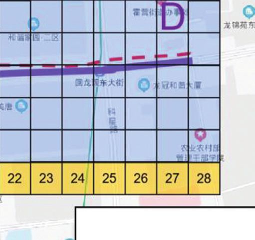
travel path. The example can be seen in Figure 3: O is the (2) 1 < i < j < n. t′i < tj′
loading position, and D is the unloading position. The
purple line represents the historical trajectory, and the red The support of the test trajectory is calculated as follows:
dotted line represents the test trajectory. The blue box in the grid coordinates (5, 2), the red trajectory and purple
represents the grid of online mapping. The yellow box trajectory are in the same grid, and the support value of the
indicates the coordinates of the grid. test trajectory is 100%. The grid coordinates (9, 5) contain
 In order to extract the spatial constraints of trajectory, only the red trajectory. The support value of the test tra-
we use part ideas of IBOAT algorithm. The specific methods jectory is 0% [29].

6 Journal of Advanced Transportation

 D

 Dt

 Ot

 O

 Figure 2: An example of OD constrained.

 normal trajectory
 abnormal trajectory

 Figure 3: An example of support (map comes from https://map.baidu.com/@12954896,4834993,13z).

 hasPath Ti , ti Definition 5 (local spatio constraint). The support con-
 support � . (3) siders the global spatial characteristics of trajectory but
 |T|
 lacks the local spatial characteristics. The trajectory is
 The support has a great influence not only on the spatial composed of trajectory points that have different effects on
anomaly detection of trajectory, but also on the temporal the abnormality of the current trajectory point. In short,
anomaly detection. The modeling of real-time temporal the closer the trajectory point is to the current test tra-
anomaly depends on the spatial anomaly detection results. jectory point, the greater the impact on the anomaly. On
In other words, temporal anomaly detection is performed the contrary, the smaller the impact. In view of this
when the space is normal. Therefore, this condition is a characteristic, this paper adds two parameters, namely, t2
strong constraint for temporally anomaly detection. (length of the maximum continuous temporal anomaly

Journal of Advanced Transportation 7

window) and t1 (length of the warning time window), to temporal frequency of all historical trajectories under a
correct the results of the spatial anomaly. (in Section 6.2, we preset size window.
will explain in more detail.) Let function c(t) be the travel temporal frequency for
 window, determined by counting the length of travel temporal
 min Nu t1 , N t2 
 Rt � 100 ∗ . (4) in window that meets the above conditions in all trajectories.
 N t2 
 p(r) � P(c(t) � r), (r > 0). (5)
 Equation (4) is the model for calculating Rt (the risk
value of the trajectory). Nu (t1 ) is the maximum number of Let M(r) be the number of windows that satisfy c(t) � r.
abnormal GPS points of the test trajectory in t1. N(t2 ) is the Let Y be the total number of windows. Then, the formula can
number of all GPS points of the test trajectory in t2. The be rewritten as
longer the t1 is, the lower the tolerance of the model, while M(r)
the shorter the t2 is, the higher the sensitivity. p(r) � . (6)
 Y
 Let f(q) be the cumulative distribution function of r.
Definition 6 (global temporal xonstraint). Since the road
network and traffic conditions are dynamic, the trajectory is f(q) � p(r)dr , (r ≥ 0), (7)
also dynamic and depends on the traffic conditions.
Therefore, the trajectories of the same loading and unloading
 Let Qk (Ti, ti) be the k-th quantile of the travel time
positions may be completely different during peak hours and
 probability distribution of the historical trajectories in the i-
other times of the day. In terms of time, we divide trajec-
 th window. We use a probabilistic method to model the
tories according to the traffic conditions in different periods.
 distribution of the travel times of historical trajectories to
Taking Beijing as an example, the morning and evening
 detect temporal anomalies in the test trajectory.
peaks are from 7:00 a.m. to 9:00 p.m. and from 5:00 p.m. to 8: 
00 p.m. Based on this, we divide the time into four periods: 7: hasPath Ti , ti 
00 am–9:00 am, 9:00 am–5:00 pm, 5:00 pm–8:00 pm, and 8: HTi � Qk Ti , ti , > θ. (8)
 |T|
00 pm–7:00 am. We look for the same time as the test
trajectory.
 Definition 9 (adjustment mechanism: local temporal win-
 dow constraint extraction based on redundant information).
Definition 7 (local temporal window constraint). The global In the anomaly detection problem, real data may occur, in
temporally constraint classifies the trajectories from the which historical trajectory (HT) travel time is greater or less
overall time, but this is not sufficient for the real-time than the new test trajectory (NTW) travel time in the i-th
anomaly detection of the trajectory. Since the global tem- window. In this case, the travel time in the (i−1)-th window
porally constraint span is too large to meet the real-time impacts the travel time in the i-th window. Therefore, we
accuracy requirements of the trajectory, the extraction of the want to eliminate this error. We define this case as follows:
local temporally constraint with a smaller span will be the the test trajectory in the window has redundant information.
key to real-time anomaly detection. This effect is significant for temporal anomaly detection,
 A window time is used in equation (4), which inspired which will lead to insufficient or overloaded historical in-
the idea of using sliding windows for temporal anomaly formation in window. These two situations directly lead to
detection. The different window sizes provide different in- the failure of constraint extraction or not. Because the travel
formation, which is beneficial in the judgment of temporal time of the (i−1)-th window affects the travel time of the i-th
anomalies. There are two types of sliding windows. One has a window, therefore, we want to eliminate this error by using a
fixed time size, but the number of grids in the window is linear equation and Definition 8.
variable; the other has a fixed number of grids in the window, Specifically, when HT is greater than NTW, if the HT
but the time is variable. This paper uses the second method, value in the i-th window is not adjusted, the information in
which is called fixed position window, because it is more the (i−1)-th window may be carried into the i-th window.
intuitive to compare the travel time of the historical tra- This causes the HT value in the i-th window to be greater
jectory and the test trajectory in the same window. than the required HT. An adjustment coefficient (rp) is
 needed in this situation.
Definition 8 (Construct Empirical Local Temporal Window HT is less than NTW in Figure 4. This is the opposite of
Constraints Based on Historical Information). According to the above situation, but it will also cause errors due to the
the travel time preference obtained from all historical tra- introduction of redundant information. Therefore, the same
jectories, travel temporal is divided into normal temporal needs to be adjusted.
and abnormal temporal. Based on the method of detecting The formula is as follows:
outliers using box plots in anomaly detection, inspired by
 HTi � HTi + rp ∗ Δtpj + rn ∗ Δtnj . (9)
this, we use quantiles as a statistical reasoning tool to de- j∈u j∈u
termine the abnormalities of travel temporal in window. In
the historical trajectory, the trajectories that meet the The difference between the travel time of the historical
conditions of Definitions 4 and 6 constitute the travel trajectory and the travel time of the test trajectory is

8 Journal of Advanced Transportation

 TW3 g1 g2 g3 g4 g5 g6 g7 g9

 t1 t2 t3 t4 t5 t8 t9 t11

 TW6 t6 t10
 Test trajectory
 t7 TW8
 TW7
 Historical
 trajectory g1 g2 g3 g4 g5 g6 g7 g8

 t1 t2 t3 t4 t5 t6 t7 t8

 TW1 :1 NTW1=0 HT1 =0 Δt1 =0 Δ Δt1 =0 TW2 :1,2 NTW2=10 HT2 =1 Δt2 =0 Δ Δt2 =0

 TW3 :1,2,3 NTW3=20 HT3 =20 Δt3 =0 Δ Δt 3 =0 TW4 :2,3,4 NTW4=20 HT4 =20 Δt4 =0 Δ Δt4 =0

 TW5 :3,4,5(7) NTW5=20 HT5 =20 Δt5 =0 Δ Δt5 =0 TW6 :3,4,5,6(7) NTW6=30 HT6 =20 Δt6 =10 Δ Δt5 =10

 TW7 :3,4,5,6,7(7) NTW7=40 HT7 =20 Δt7 =20 Δ Δt7 =10 TW8 :3,4,5,6,7(7) NTW8=40 HT8 =20 Δt8 =20 Δ Δt8 =0

 TW9 :7,8,9(10) NTW9=20 HT9 =20 Δt9 =0 Δ Δt9 =-20 TW10 :7,8,9,10 NTW10=30 HT10 =20 Δt10 =10 Δ Δt9 =10

 Figure 4: Example of trick.

 Δti � NTWi − HTi . (10) greater than 0 are abnormal, which are marked in red; the
 locations where ΔΔti is less than or equal to 0 are normal and
 In equation (10), HTi indicates the value of k-th quantile are marked in blue. Black indicates a normal value.
for travel time in i-th window.
 Trick (relaxation for HT less than NTW): The case where Definition 10 (constructing empirical average speed ratio
HT is greater than or less than HTW has different effects on constraint). The change in average speed can express the
abnormal judgment. More precisely, when HT is greater change in travel time well. Therefore, the speed is referenced
than NTW, it means that the test trajectory is normal, but the to help filter out the temporal anomaly in equation (6),
redundant value will affect the abnormal judgment of the where a is the speed ratio threshold, and WTR is the speed
next point. When HT is less than NTW, the test trajectory is ratio of the i-th window. When WTR is greater than a, the
abnormal. This is a situation where we need to detect time travel time of the i-th window is abnormal. The formula is as
anomalies. At this time, the estimation accuracy of the re- follows:
dundant value is fatal to the result of abnormal judgment, so 
 speed Q hasPath T , t /|T| < θ − speed NTW 
we try to relax the constraint at this time. Figure 4 shows this 3 i i i 
 WTRi � > α.
trick method. An example is given to illustrate the above speed Q3 hasPath Ti , ti /|T| < θ 
method. Figure 4 shows the calculation results of this (11)
method when the window size is 3.
 In Figure 4, HTrepresents the travel time of the historical
trajectory. The digital value of HT represents the time Definition 11 (travel time of the test trajectory). NTW is the
step—a time step is 10 seconds—and the grid represents the travel time of the test trajectory, which is equal to the length
location of the vehicle. NTW is the travel time of the test of the window minus 1.
trajectory in the window. TWi is the i-th window; Δti is the NTWi � len TWi − 1 . (12)
difference between NTW and HT, which represents the
difference between the travel time of the test trajectory and The above description is called window time of isolation
the historical trajectory. ΔΔti is the difference between Δti based online anomalous trajectory detection (WT-iBOAT)
and Δti−1 . In Figure 4, TW8 is a special window. Time Step 4 algorithm, which adds an abnormal temporal detection
is followed by time Step 7 in TW8 in the test trajectory, which method to iBOAT [29]. Algorithm 1.
means that time steps (5, 6, 7) are in the same grid. There is The pseudocode of WT-iIBOAT algorithm is as follows:
30 seconds between time Step 4 and time Step 7. Time Step 4
is followed by time Step 5 in TW8 in the historical trajectory, 4. Results
which means that only 10 seconds elapses. If NTW and HT
are directly compared at TW8, this will lead to an incorrect 4.1. Data Description. To detect abnormal trajectories of
conclusion. Through observation, we discover that this in- urban freight vehicles, the historical trajectories provided by
correct conclusion is caused by time steps 5, 6, and 7 in TW8 a logistics company in Beijing were used in this paper.
in NTW. However, by comparing ΔΔti , this problem can be The data were collected from approximately 35 vehicles
solved. The value of ΔΔt8 is 0, and the value of ΔΔt9 is (−20). in Beijing in 2019 (September to October 2019). The main
Finally, we obtain the rule that the locations where ΔΔti is fields are the vehicle status, longitude, latitude, offset

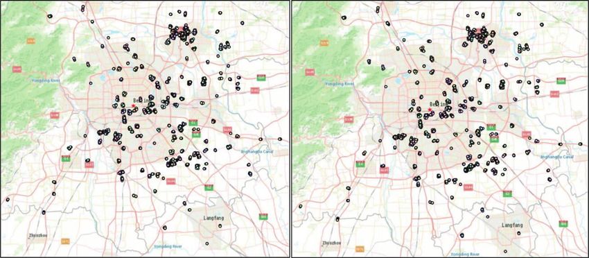
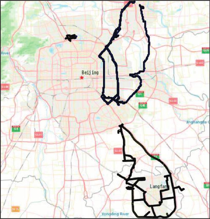
Journal of Advanced Transportation 9

 Input:i: input point index,
 WL: window time step,
 T: historical trajectory dataset,
 θ: spatial anomaly threshold,
 α: temporal anomaly threshold
 Output X: abnormal trajectory points,
 Rti : the risk value of the trajectory
 Process:
 (1) While new grid received from online gridding
 (2) support(i) � hasPath(Ti−1 , ti )/Ti−1
 (3) if support(i) < θ:
 (4) X←update(support(i))
 (5) Ti ←updata(hasPath(Ti−1 , ti ))
 (6) else:
 (7) HTi ←Q3 (|hasPath(Ti , ti )|/|T| < θ)
 (8) HTi � update(HTi , Δtpj , Δtnj , r)
 (9) NTWi ←calculate(celli , celli−t )
 (10) Δti ←calculate(NTWi , HTi )
 (11) ΔΔti ←calculate(Δti , Δti−1 )
 (12) if WTRi > α and ΔΔti > 0:
 (13) X←update(WTRi , ΔΔti )
 (14) end if
 (15) end if
 (16) Rti ←calculate(count(XWL ), count(WL))
 (17) end while

 ALGORITHM 1: WT-iBOAT.

dimension, city code, working condition time, GPS time, data, including the visualization of the trajectory data, the
accumulated mileage, positioning status, vehicle speed, ve- travel time distribution, and the travel distance distribution.
hicle ID, etc. It should be noted that these data are recorded To analyze the performance of the spatial anomaly de-
every 10 seconds. We first need to segment the raw trajectory tection of the algorithm, we manually mark all trajectories
according to the business requirements of logistics. There- and then calculate the accuracy of the algorithm. The per-
fore, loading and unloading points that are common loca- formance analysis of temporal anomaly detection uses the
tions for vehicles to load and unload goods are used as the method of comparing the different window sizes.
segmentation points of the trajectory. Loading and Figures 7 and 8 show visualizations of spatiotemporal
unloading points are obtained by the effective parking time anomalies using a hot map. The hot map, which uses dif-
of the vehicle. The effective parking time depends on the ferent colors to indicate statistically abnormal values, is
experience of the staff. The regularity of vehicle trajectory generated by counting the number of anomalous grids in the
can be found by the loading and unloading position obtained window on a test trajectory. The red points are GPS points,
from the effective parking time. Clustering is a good choice which represent the travel route of the vehicle. Figure 8
to obtain this regularity. DBSCAN [33] is a density based displays only the nonabnormal routes.
algorithm, which assumes that the category can be deter-
mined by the compactness of the sample point distance.
 DBSCAN is commonly used to find the loading and 4.2. Results of Spatial Anomaly Detection. In Figure 7, dif-
unloading positions. The parameters of the algorithm are ferent spatial anomalies are highlighted. The normal tra-
minimum number of fields (MINPTS) � 60 and domain jectories are almost the shortest routes between the loading
radius (EPS) � 150 meters. A total of 151 loading position and unloading positions. An analysis of each picture is given
categories and 151 unloading position categories are ob- below. In Figure 7(a), a route with more serious spatial
tained. The clustering results based on the ArcGIS platform anomalies chooses the East 4th Ring Expressway instead of
are shown in Figure 5. On the left is the loading position, and the East 5th Ring Expressway. There are 106 trajectories in
on the right is the unloading position. The loading and this dataset, 6 of which are on this route. Through map
unloading positions in the central city are relatively con- matching, it is found that these trajectories do not leave the
centrated, which meets the requirements of urban logistics, East 4th Ring Expressway. Therefore, these abnormalities
indicating that the clustering results reflect the common may be caused by the driver’s negligence, which leads to a
working area. failure to change lanes in time and a missed opportunity to
 By screening the above loading and unloading positions, enter the 5th Ring Expressway. In Figure 7(b), there are
three trajectory datasets with relatively good quality are some locations with serious abnormalities and concentrated
finally selected to test the algorithm. Figure 6 describes the areas. This may be due to vehicles with temporary

10 Journal of Advanced Transportation

 Figure 5: Clustering results of the loading and unloading points (map comes from https://www.tianditu.gov.cn/).

 40–60

 41.6%

 0–40
 8.4%

 7.2%
 >120

 29.4% 13.4%

 90–120
 60–90

 0–40
 40–60
 60–90
 90–120
 >120

 (a) (b)

 80

 60
 Trajectory of Number

 40

 20

 0

 5 10 15 20 25 30 35 40 45 50 55 60 65 70 75 80 85 90 95 100
 Distance (km)

 count

 (c)

Figure 6: Data description (map comes from https://www.tianditu.gov.cn/). (a) Visualization. (b) Travel time distribution. (c) Travel
distance distribution.

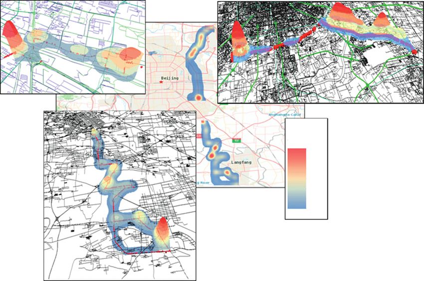
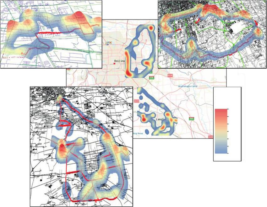
Journal of Advanced Transportation 11

 (c) (a)

 12
 10
 8
 6
 4
 2
 0

 (b)
Figure 7: Spatial anomaly distribution (map comes from https://www.tianditu.gov.cn/, the number of legends in the figure is to facilitate the
visualization of abnormal results, so the calculation results of spatial anomalies are divided into 12 levels.).

transportation tasks. In Figure 7(c), the purpose of detouring Guangming West Road and Xichang Road in Langfang city
vehicles may be to avoid large intersections. However, has a large traffic volume and is prone to traffic congestion.
Figure 8(c) shows that there are not many temporal Figure 8(c) shows the Shangqing Bridge in Beijing city. The
anomalies at the intersection. Instead, there is a temporal figure shows that temporal anomalies mostly occur on the
anomaly on the street near the destination. Therefore, it is roads approaching adjacent residential areas and at inter-
reasonable that the vehicle is avoiding possible traffic jams changes (such as the intersection with Shangqing Bridge),
on that street. which is consistent with the actual situation.
 The above analysis describes the reasons for spatio-
 temporal anomalies under different conditions. It is dem-
4.3. Results of Temporal Anomaly Detection. In Figure 8, red onstrated that the anomaly detection algorithm proposed in
represents abnormally severe areas in terms of anomalies, this paper can address actual situations.
and blue represents abnormally mild areas. From Figure 8, it
can be concluded that most of the abnormal areas are close
to the intersection, and the areas close to the starting and 4.4. Results of Abnormal Trajectory Detection. Finally, a
ending points are more likely to be abnormal. trajectory is used for qualitative analysis to present all the
 In Figure 8(a), the temporal anomalies mainly occur at results of the algorithm. Figure 9 shows a trajectory with ID
the intersection of Beijing Shenyang Road and Huosha Road 27636. The spatial shape of this trajectory is shown in
and at the intersection of Beijing Shenyang Road and the Figure 9(a). The blue points are normal, and the red points
airport expressway. A road with almost no temporal are abnormal.
anomalies is the East 5th Ring Expressway. The temporal Figures 9(b)–9(d) display the temporal anomalies, spatial
anomalies in Figure 8(b) mainly occur in the suburbs be- anomalies, and risk value of the trajectory, respectively.
tween Hebei Province and Beijing city and at the intersection Figure 9(d) expresses all the spatiotemporal anomaly in-
of Guangming West Road and Xichang Road in Langfang formation. A change in color indicates a change in the
city. In the suburbs between Hebei Province and Beijing, the density of the temporal (Figure 9(b)) and spatial
roads pass through settlements, and temporal anomalies (Figure 9(c)) anomalies in t1 of equation (1). From
occur in dense residential areas. The intersection of Figure 9(d), we can identify anomalous trajectory segments

12 Journal of Advanced Transportation

 (c)
 (a)

 12
 10
 8
 6
 4
 2
 0

 (b)
Figure 8: Temporal anomaly distribution (map comes from https://www.tianditu.gov.cn/, The number of legends in the figure is to facilitate
the visualization of abnormal results, so the calculation results of temporal anomalies are divided into 12 levels).

and determine a level of risk to warn of the potential security of normal trajectories. The right y-axis is the processing time.
risk. Figure 9(d) is the concept of risk value calculated A representative dataset is selected considering the long
according to equation (4). Users can define the risk level transport distance of urban freight vehicles. There are 106
according to their own needs according to different value of trajectories in this dataset, of which 99 are normal and 7 are
risk. In equation (4), t1 and t2 can be adjusted according to abnormal. Figure 10 shows that when using a 250 m × 250 m
the varied demand of different scenarios. grid, most normal trajectories were found, and the pro-
 cessing time was at a high level. Therefore, 250 m is selected
 for spatial anomaly detection.
5. Analysis
This section comprehensively analyzes the impact of dif-
ferent parameters on accuracy and analyzes the differences 5.2. Temporal Anomaly Parameter Analysis. For temporal
between our proposed method and iBOAT and TRAOD anomaly detection, manual methods are not used, because it
algorithms. After that, the results of the three methods are is difficult for manual methods to find a reasonable standard
explained on our data. to judge when and where the GPS points are abnormal.
 Environment: our algorithm is mainly implemented in Therefore, we observe the impact for other window sizes,
Python. The machine used for the experiment has a 9th with the result of window size � 2 as the benchmark, and we
generation i7 CPU and 32 G memory. The operating system conduct a contrastive analysis to explain the feasibility and
is Windows 10 x86_64, and the compiler is Spyder 4.15. advantages of the algorithm proposed in this paper.
 Figure 11(a) shows the method, where the x-axis represents
 time and the y-axis represents space. Spaces 5 to 3 (the
5.1. Spatial Anomaly Parameter Analysis. Spatial anomaly window is 2) are used as a benchmark to judge the algo-
detection for vehicles focuses mainly on the impact of the rithm’s performance under different parameters, e.g., spaces
grid size on accuracy and processing time. Figure 10 displays 5 to 1 (the window is 4). Next, we will analyze the per-
these results. In Figure 10, the blue line represents the impact formance and accuracy of WT-iBOAT.
of the grid size on the accuracy, and the red line shows the Performance: Figure 11(b) shows the processing time of
impact of the grid size on the processing time of the pro- WT-iBOAT and iBOAT. The processing time of WT-iBOAT
gram. The x-axis is the grid size. The left y-axis is the number is approximately 2.5 times that of iBOAT. It does not change

Journal of Advanced Transportation 13

 1.0 0 1.0
 280 7 0.8
 14
 21 0.6
 28 0.4
 260 35
 0.8 42 0.2
 49 0.0

 0
 5
 10
 15
 20
 25
 30
 35
 40
 45
 50
 55
 60
 65
 70
 75
 80
 85
 90
 95
 100
 105
 110
 115
 120
 125
 130
 135
 140
 145
 150
 155
 160
 165
 170
 175
 180
 185
 190
 195
 200
 205
 210
 215
 220
 225
 230
 235
 240
 245
 250
 255
 260
 265
 270
 275
 280
 285
 290
 295
 300
 305
 240

 0.6
 220

 200 0.4

 180
 0.2
 160

 0.0
 150 160 170 180 190 200

 (a) (b)
 0 1.0
 7 0.8
 14
 21 0.6
 28 0.4
 35 0.2
 42
 49 0.0
 0
 5
 10
 15
 20
 25
 30
 35
 40
 45
 50
 55
 60
 65
 70
 75
 80
 85
 90
 95
 100
 105
 110
 115
 120
 125
 130
 135
 140
 145
 150
 155
 160
 165
 170
 175
 180
 185
 190
 195
 200
 205
 210
 215
 220
 225
 230
 235
 240
 245
 250
 255
 260
 265
 270
 275
 280
 285
 290
 295
 300
 305
 (c)
 0 0.75
 7 0.60
 14
 21 0.45
 28 0.30
 35
 42 0.15
 49 0.00
 0
 5
 10
 15
 20
 25
 30
 35
 40
 45
 50
 55
 60
 65
 70
 75
 80
 85
 90
 95
 100
 105
 110
 115
 120
 125
 130
 135
 140
 145
 150
 155
 160
 165
 170
 175
 180
 185
 190
 195
 200
 205
 210
 215
 220
 225
 230
 235
 240
 245
 250
 255
 260
 265
 270
 275
 280
 285
 290
 295
 300
 305
 (d)

Figure 9: Risk value analysis. (a) Original trajectory. Blue represents the normal value, and red represents the abnormal value. (b) The
temporal abnormal trajectory. (c) The spatial abnormal trajectory. (d) The risk value calculated according to formula (4).

 90 300 travel times of trajectories that are classified as normal; true
 275 negatives (TN) are the number of anomalous travel times of
 80 trajectories that are classified as normal; and false negatives
 250
 (FN) are the number of normal travel times of trajectories
accuracy rate

 70
 225 that are classified as anomalous. We report these cases and
 Time

 60 200 calculate the common metrics of precision, true positive rate
 (TPR), defined as TPR � TP/TP + FN, and true negative rate
 50 175
 (TNR), defined as TNR � (TN/TN + FP). A perfect classifier
 40 150 will have TNR � 1 and TPR � 1.
 125 In Figure 12(a), window size ≤ 6, quantile � 75,
 100 150 200 250 300 350 400 TPR > 0.75; in Figure 12(b), quantile > 75, window size � 4,
 size of grid and TPR > 0.825. This reflects that as long as the parameter
 accuracy rate
 settings are reasonable, our algorithm can achieve relatively
 Time excellent results. To be more specific, when considering the
 effect of the window size on accuracy, the quantile is de-
 Figure 10: Abnormal spatial detection performance analysis. termined to be 75. This is because when the quantile is 75,
 there is a higher requirement for the travel time, which is
 convenient for comparing the results of the algorithms. The
with the number of historical trajectories. This shows that 75th quantile and the 2 windows are selected as the target
the processing time is stable, and the processing time of each values. Figure 12(a) plots the results with regard to different
GPS point is approximately 0.006 seconds. Therefore, the values of window size. TPR decreases rapidly with increasing
algorithm can be used for real-time detection. window size, which indicates that the larger the window size
 Accuracy: the travel time of a trajectory will fall into one is, the longer the travel time allowed by the window, so the
of four cases: true positives (TP) are the number of proportion of positive sample detections decreases. Quan-
anomalous travel times of trajectories that are classified as tifying TPR, when the window sizes are 3, 4, 5, 6, 7, 8, 9, and
anomalous; false positives (FP) are the number of normal 10, the TPR calculated by the algorithm is 87%, 82.5%, 78%,

14 Journal of Advanced Transportation

 1600
 1400
 5
 1200

 Processing Time
 4 1000
 800
 Space

 3
 600
 2 400
 200
 1
 0
 1 2 3 4 5 6 7

 11098

 18414

 22196

 33294

 36828

 44392

 55242

 55490

 73656

 92070
 Time

 Size of Data
 I BOAT
 WT–I BOAT
 (a) (b)

 Figure 11: (a) Example of temporal anomaly parameter analysis. (b) Processing time of WT-iBOAT and iBOAT.

 1.00 1.000
 0.975
 0.95
 score of Window size

 0.950
 score of Quantile

 0.90
 0.925
 0.85 0.900

 0.80 0.875
 0.850
 0.75
 0.825

 2 3 4 5 6 7 8 9 10 70 75 80 85 90 95
 Window size Quantile

 TPR TPR
 TNR TNR
 (a) (b)

Figure 12: The effect of the window and quantile on accuracy. (a) The effect of the window on accuracy. (b) The effect of the quantile on
accuracy.

77%, 75%, 74%, 72%, and 71% of the benchmark, anomaly detection occurs. Specifically, the TPR of 4 win-
respectively. dows and 70th quantile is 82% of that of 2 windows and 70th
 However, TNR hardly declines, indicating that the quantile; the TPR of 4 windows and 75th quantile is 82% of
window has little impact on the judgment of negative that of 2 windows and 75th quantile; the TPR of 4 windows
samples, which is actually the role of the adjustment and 80th quantile is 85% of that of 2 windows and 80th
mechanism in the algorithm. The adjustment mechanism quantile; the TPR of 4 windows and 85th quantile is 87.5% of
effectively reduces the impact of previous moments in the i- that of 2 windows and 85th quantile; the TPR of 4 windows
th window. and 90th quantile is 91.5% of that of 2 windows and 90th
 When studying the impact of the quantiles on accuracy, quantile; the TPR of 4 windows and 95th quantile is 95% of
the window size is chosen as 4, because this is an obvious that of 2 windows and 95th quantile.
turning point in Figure 12(a). This shows that enough in-
formation is considered in 4 windows. Figure 12(b) shows
that TPR and TNR increase with increasing quantiles. This 5.3. Abnormal Trajectory Detection and Analysis. In order to
means that the higher the tolerance is, the less temporal illustrate the algorithm more effectively, we compare our

Journal of Advanced Transportation 15

 Table 2: Comparison of abnormal trajectory results.
 WT-iBOAT iBOAT TRAOD
WT-iBOAT 48 13 11
iBOAT 13 13 4
TRAOD 11 4 39
Spatial anomaly 13 13 39
Temporal anomaly 35 0 0

algorithm with the TRAOD algorithm and iBOAT algorithm 6.1. Overall Discussion of the Adjustment Mechanism. For the
in the case study. TRAOD is an offline algorithm, which can overall discussion of the adjustment mechanism, the
get abnormal trajectories by clustering the segments of speed ratio can explain the information of the window
different trajectories [8]. The TRAOD algorithm has high well. If speed ratio > 0, the travel time is abnormal. If
efficiency on finding out the trajectories with more lane speed ratio < 0, the travel time is normal. The larger the
changes. The results are as follows: in 212 trajectories, our speed ratio is, the more serious the temporal anomaly,
method found all 48 abnormal trajectories, while iBOAT and the smaller the speed ratio is, the milder the temporal
algorithm only found 13 abnormal trajectories, and anomaly. The following case needs to be explained: when
TRAOD algorithm found 39 abnormal trajectories. the test trajectory immediately turns a spatial anomaly
Among them, 11 of the 48 abnormal trajectories found by into a temporal anomaly, the travel time of the historical
our method are the same as 11 of the 39 abnormal tra- trajectory is zero, and the speed ratio is infinite. To detect
jectories found by TRAOD, of which 4 belong to spatial this, when calculating the speed ratio, greater sensitivity
anomaly and 7 belong to temporal anomaly. iBOAT and is required. Therefore, the historical speed is taken as
TRAOD have the same four spatial anomaly trajectories. 50 m/s, so the first speed ratio is equal to (50-250/10)/
All the 13 abnormal trajectories found by iBOAT algo- 50 � 0.5, and the subsequent speed ratio will also be
rithm are in 48 trajectories found by our method. The greater than 0.5.
results are shown in Table 2. Figure 13 is the kernel density diagram of the abnormal
 The reason for getting such different results is that the speed ratio of all datasets. The green, yellow, black, and blue
principle of the TRAOD algorithm is different from that of areas are the kernel density diagrams of the 75th quantile
our algorithm. TRAOD algorithm needs to cut the tra- with a window of 4, the 90th quantile with a window of 4, the
jectory into segments and then classify the trajectory 75th quantile with a window of 8, and the 90th quantile with
segments. Then, the TRAOD algorithm uses the weighted a window of 8, respectively. The first row is the kernel density
sum of vertical distance, parallel distance, and angular diagram without the adjustment mechanism, and the second
distance to calculate the distance between track segments. row is the kernel density diagram with the adjustment
This makes the algorithm very sensitive to parameters, mechanism.
and the results of different parameters will be quite Note that the different color areas in the first row are
different. more dissimilar than their counterparts in the second row.
 The outliers obtained by our algorithm are mainly This shows that the adjustment mechanism makes the ab-
determined by the travel time of vehicles in the time normal speed ratio more reasonable in different situations.
window, while the outliers obtained by TRAOD algorithm The adjusted results tend to be more concentrated in areas
are mainly determined by the distance between the tra- with smaller speed ratios, and the larger areas are reduced
jectory segments. This leads our algorithm to pay more accordingly, which is a manifestation of the rationality of the
attention to the travel speed of vehicles, and the TRAOD adjustment.
algorithm to pay more attention to the anomaly caused by
lane change.
 At the same time, a serious disadvantage of the TRAOD 6.2. Improved Analysis of Spatial Anomaly. The algorithm
algorithm is that it takes a long time to adjust parameters and judges whether the test trajectory is a spatial anomaly by
needs different parameters for different data. In our three calculating the support values. However, simply using the
datasets, we use three groups of different parameters to judge support values causes errors due to the grid. Figure 14 shows
the trajectory anomaly of the TRAOD algorithm. This may the results of the problem and improvement. The different
highlight the advantages of our method with respect to colors in the left figure represent different support values.
TRAOD algorithm in practical use. Red represents larger support values, and blue represents
 smaller support values. In the green box, when the grid size is
 250 × 250 meters, a normal spatial point may be judged as an
6. Discussion abnormal point. Section 4 equation (1) can be used to solve
 this problem. The right figure shows the result of using this
In this section, we discuss the role of the adjustment formula when t2 is 10 minutes and t1 is 3 minutes. The right
mechanism in the algorithm. Then, an example is used to figure reflects the correction of the calculation results very
explain how equation (1) improves the results of spatial well. Blue indicates a low abnormality, and red indicates a
anomaly detection. high abnormality.

16 Journal of Advanced Transportation

 3.0
 2.0 2.5 2.0
 1.5 2.0 1.5
 1.0 1.5 1.0
 1.0
 0.5 0.5 0.5
 0.0 0.0 0.0
 –0.2 0.0 0.2 0.4 0.6 0.8 1.0 1.2 –0.2 0.0 0.2 0.4 0.6 0.8 1.0 1.2 –0.2 0.0 0.2 0.4 0.6 0.8 1.0 1.2
 75, N, 4 75, N, 8 75, N, 4 75, N, 8 75, N, 4 75, N, 8
 90, N, 4 90, N, 8 90, N, 4 90, N, 8 90, N, 4 90, N, 8

 2.5 4.0 2.0
 2.0
 3.0 1.5
 1.5
 2.0 1.0
 1.0
 0.5 1.0 0.5
 0.0 0.0 0.0
 –0.2 0.0 0.2 0.4 0.6 0.8 1.0 1.2 –0.2 0.0 0.2 0.4 0.6 0.8 1.0 1.2 –0.25 0.0 0.25 0.5 0.75 1.0 1.25
 75, Y, 4 75, Y, 8 75, Y, 4 75, Y, 8 75, Y, 4 75, Y, 8
 90, Y, 4 90, Y, 8 90, Y, 4 90, Y, 8 90, Y, 4 90, Y, 8
 Figure 13: Overall analysis of the adjustment mechanism.

 1.0 1.0
 40.045 40.045

 40.040 0.8 40.040 0.8

 40.035 40.035
 0.6 0.6
 40.030 40.030
 Lat

 Lat

 40.025 0.4 40.025 0.4
 40.020 40.020
 0.2 0.2
 40.015 40.015

 40.010 40.010
 0.0 0.0
 116.33 116.34 116.35 116.36 116.37 116.33 116.34 116.35 116.36 116.37
 Ing Ing

 Figure 14: Improved analysis of spatial anomalies.

7. Conclusion results calculated by our method is more practicable as
 explained in Section 6.1. It is fairly acceptable that the FPR is
Taking trajectory security as the research background, this increased by only 0.013 with 22.5% more anomalies correctly
paper provides an effective real-time risk monitoring scheme detected. Therefore, the result proves that our proposed
for detecting the anomalous trajectory of logistics vehicles. algorithm can effectively detect the abnormal trajectories of
The main idea is to combine the spatial and temporal urban freight vehicles in real time with not only higher
anomaly detection by using the time probability distribution accuracy, but also lower false alarm rate. This can provide
of historical trajectory and taking the fixed position window more efficient, faster, and safer logistics express services for
as the detection fragment. addressing unexpected trajectory anomaly events.
 The results show that the algorithm can achieve higher There are still some deficiencies in the current research.
accuracy, and the risk detection reaches 82.5% of the For example, when the historical trajectory data set is large,
benchmark on our dataset, outperforming the traditional the real-time query of historical data will cost a lot of cal-
iBOAT algorithm (60%). At the same time, the false positive culation, and the probability model will help solve this
rate (FPR) of iBOAT is 0.031, and the FPR of our method is problem. Further research can establish probability model or
0.044. Comparing the FPR values of the two methods, the neural network for different data to improve the speed of
higher FPR value of our method is caused by the supple- discovery from different start and end points.
mented temporal anomaly detection. However, we suc- In general, (1) the framework we use can be reasonably
cessfully found 22.5% more anomalies than iBOAT and widely applied to security service scenarios for urban
algorithm by using adjustment mechanism in temporal freight vehicles. (2) For temporal anomalies, we propose a
anomaly, so that the distribution of temporal anomaly simple, fast, and efficient real-time temporal anomaly