Active Flows on Curved Surfaces - TU Dresden
←
→
Page content transcription
If your browser does not render page correctly, please read the page content below
This draft was prepared using the LaTeX style file belonging to the Journal of Fluid Mechanics   1

                                                                Active Flows on Curved Surfaces
arXiv:2102.03098v1 [physics.flu-dyn] 5 Feb 2021

                                                                                M. Rank1 and A. Voigt1,2,3 †
                                                           1
                                                            Institut für Wissenschaftliches Rechnen, TU Dresden, 01062 Dresden, Germany
                                                  2
                                                      Center for Systems Biology Dresden (CSBD), Pfotenhauerstr. 108, 01307 Dresden, Germany
                                                            3
                                                              Cluster of Excellence - Physics of Life, TU Dresden, 01062 Dresden, Germany

                                                                                (Received xx; revised xx; accepted xx)

                                                  We consider a numerical approach for a covariant generalised Navier-Stokes equation on
                                                  general surfaces and study the influence of varying Gaussian curvature on anomalous
                                                  vortex-network active turbulence. This regime is characterised by self-assembly of finite-
                                                  size vortices into linked chains of anti-ferromagnet order, which percolate through the
                                                  entire surface. The simulation results reveal an alignment of these chains with minimal
                                                  curvature lines of the surface and indicate a dependency of this turbulence regime on the
                                                  sign and the gradient in local Gaussian curvature. While these results remain qualitative
                                                  and their explanations are still incomplete, several of the observed phenomena are in
                                                  qualitative agreement with experiments on active nematic liquid crystals on toroidal
                                                  surfaces and contribute to an understanding of the delicate interplay between geometrical
                                                  properties of the surface and characteristics of the flow field, which has the potential to
                                                  control active flows on surfaces via gradients in the spatial curvature of the surface.

                                                  Key words: active turbulence, generalised Navier-Stokes equation, toroidal surface

                                                  1. Introduction
                                                     To model fluids on curved surfaces is a problem which dates back to Scriven (1960),
                                                  who derived a covariant Navier-Stokes (NS) equation and established the coupling
                                                  between spatial curvature and fluid flow. The influence of geometric properties on both,
                                                  equilibrium configurations and the dynamics far from it, has consequences in a huge
                                                  variety of problems, ranging from planetary flows (Delplace et al. 2017) to active nematic
                                                  films on vesicles (Keber et al. 2014). Further examples, where the spatial curvature
                                                  influences fluid flow, are found in developmental biology, e.g. tissue morphogenesis
                                                  (Heisenberg & Bellaiche 2013), cell division (Mayer et al. 2010) and biochemical signal
                                                  propagation (Tan et al. 2020), biofilm formation (Chang et al. 2015) and bacterial
                                                  colonization (Sipos et al. 2015). All these examples offer the possibility to influence or
                                                  even control fluid flow by the spatial curvature of the surface.
                                                     The resulting huge interest in surface flows is in contrast to a still missing coherent
                                                  theoretical understanding of the interplay with geometric properties. Analytical results
                                                  in oversimplified situations are of limited value in this context and also numerical
                                                  approaches were until recently restricted to special cases. Most of them are based on
                                                  a vorticity-stream function formulation (Nitschke et al. 2012; Reuther & Voigt 2015;
                                                  Gross & Atzberger 2018; Reusken 2020) and have been applied to surface Stokes or NS
                                                  equations. More recently they are also considered simulating active flows on surfaces
                                                                   † Email address for correspondence: axel.voigt@tu-dresden.de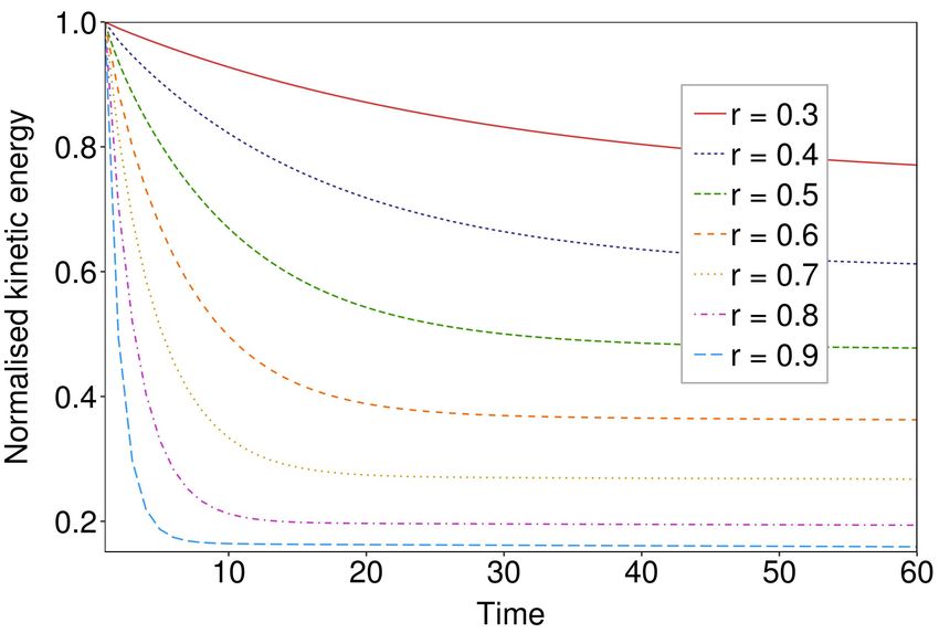
2                                  M. Rank and A. Voigt
(Pearce et al. 2019; Torres-Sanchez et al. 2019; Supekar et al. 2020). The advantage
of the vorticity-stream function formulation is the avoidance of tangential vector fields.
This allows to explore well-established numerical methods for scalar fields on surfaces.
However, in contrast to the Euclidian setting, the Helmholtz-Hodge decomposition - see
Bhatia et al. (2013) for a review - which provides the mathematical basis for the vorticity-
stream function formulation, not only splits the tangential velocity field into curl-free and
divergence-free components, but might also contain non-trivial harmonic vector fields -
vector fields which are curl- and divergence-free. Their richness depends on the topology
of the surface (Jost 1991). As these vector fields cannot be described by the vorticity-
stream function formulation, the approach is only applicable for surfaces, where harmonic
vector fields are trivial, which are only simply-connected surfaces (Nitschke et al. 2020b).
Reuther & Voigt (2018) and Fries (2018) introduce a numerical approach for a surface
NS equation in its velocity-pressure formulation, which is applicable on general surfaces.
The underlying idea was independently introduced in Nestler et al. (2018), Jankuhn et al.
(2018) and Hansbo et al. (2020) and is described in detail in Nestler et al. (2019). It relies
on an extension to an embedding thin film. This allows to express the covariant derivatives
in terms of partial derivatives along the Euclidian basis. The surface partial differential
equation can thus be solved by considering each component by established methods for
scalar quantities and enforcing the normal contributions to be zero, either by penalisation
or by Lagrange multipliers. Also this approach has been applied to active flows in the
context of surface active polar gels (Nitschke et al. 2019). Other numerical approaches for
the surface Stokes or NS equation, directly acting on the tangential velocity and pressure
fields, are proposed in Nitschke et al. (2017), Torres-Sanchez et al. (2020), Sahu et al.
(2020) and Lederer et al. (2020).
   We will here consider a modelling approach for active flows and extend studies for a
generalised Navier-Stokes (GNS) equation on a sphere (Mickelin et al. 2018) to toroidal
surfaces. This GNS equation describes internally driven flows through higher-order
hyperviscosity-like terms in the stress tensor. In flat space such models have been
phenomenologically proposed for active fluids (Wensink et al. 2012) with additional
Toner-Tu like terms (Toner & Tu 1998) and later on have been justified by microscopic
theories (Heidenreich et al. 2016). The proposed version in Slomka & Dunkel (2015,
2017) focuses on the solvent velocity field. Under the assumption of dense suspensions
this allows to neglect the local driving terms and additional active stresses and describe
the active flow solely by a generalised stress tensor, which comprises passive contributions
from the intrinsic solvent fluid viscosity and active contributions representing the stresses
exerted by the active components on the fluid. The version in Slomka & Dunkel (2015,
2017) can also be derived from classical hydrodynamic models with active stresses
(Linkmann et al. 2020b). The model serves as a minimal model for active fluids and
had been successful in reproducing active turbulence flow patterns of swimming bacteria,
ATP-driven microtubules and artificial microswimmers, see, e.g. (Bratanov et al. 2015;
James et al. 2018) and had also been studied previously for seismic wave propagation
(Beresnev & Nikolaevskiy 1993; Tribelsky & Tsuboi 1996). Investigations on surfaces are
so far restricted to spherical surfaces (Mickelin et al. 2018; Supekar et al. 2020). The
considered numerical approach uses a pseudo-spectral method with a basis of spherical
harmonics. Besides the restriction of this approach to a sphere, also the constant Gaussian
curvature in this case implies that only the size of the sphere matters. Non of these
approaches is applicable to general surfaces.
   Results on the influence of varying Gaussian curvature on active flows are rare. Besides
a few microscopic models for active nematics, which do not account for hydrodynamic
effects (Alaimo et al. 2017; Apaza & Sandoval 2018; Ellis et al. 2018), continuum models,
Active flows on curved surfaces                              3
with numerics based on the vorticity-stream function formulation (Torres-Sanchez et al.
2019; Pearce et al. 2019) and the generally applicable approach for polar liquid crystals
(Nitschke et al. 2019) as well as first experimental work on active nematic liquid crystals
comprised of microtubules and kinesin, which are constrained to lie on a toroidal surface
(Ellis et al. 2018), no results are available. The last is especially interesting as it
has regions with both positive and negative Gaussian curvature. From equilibrium
considerations it is expected that topological defects in the nematic liquid crystal, here
of charge ± 21 , are attracted by regions of like-sign Gaussian curvature. A phenomenon
which has been explored in detail for disclinations in positional order (Bowick et al. 2004;
Giomi & Bowick 2008) and is expected to carry over to orientational order (Turner et al.
2010; Jesenek et al. 2015). The experiments in Ellis et al. (2018) suggest that active
flows on surfaces can be guided and controlled via gradients in the spatial curvature of
the surface. They show that pairs of defects unbind and segregate in regions of opposite
Gaussian curvature. At least qualitatively these results have been reproduced in Pearce
et al. (2019), showing a linear dependency of defect creation and annihilation rates on
Gaussian curvature. As these rates are directly linked to active turbulence (Giomi 2015),
a connection between spatial curvature and active turbulence can be expected. Pearce
et al. (2019) consider an active nematodynamics model which is based on a simplified
surface Landau-de Gennes energy (Kralj et al. 2011). For more detailed surface Landau-
de Gennes models which also take extrinsic curvature contributions into account, see
Golovaty et al. (2017), Nitschke et al. (2018) and Nestler et al. (2020). As already pointed
out, the numerical treatment in Pearce et al. (2019) is based on a vorticity-stream function
formulations, which is inappropriate for toroidal surfaces. Appropriate numerical studies
for active nemotodynamics on general surfaces are still under development. However,
several open questions, e.g., the influence of spatial curvature on active turbulence can
already be studies using an appropriately coarse-grained mesoscopic GNS equation.
   Here we focus on one aspect of the active flow. We only consider the influence of spatial
varying curvature on anomalous vortex-network active turbulence. The simulations in
Mickelin et al. (2018) on a sphere reveal a global curvature-induced transition from
a quasi-stationary burst phase to an anomalous vortex-network turbulent phase and
a classical 2D Kolmogorov turbulent phase. The new type of anomalous turbulence
is characterised by the self-assembly of finite-size vortices into linked chains of anti-
ferromagnetic order, which percolate through the entire fluid domain. The coherent
motion of this vortex chain network provides an upward energy transfer and thus an
alternative to the conventional energy cascade in classical 2D hydrodynamic turbulence.
We will answer the question if this mechanism is altered by gradients in curvature by
considering the GNS equation on different tori within a parameter setting which leads
to anomalous vortex-network turbulence on a sphere.
   The paper is organised as follows: In Section 2 we introduce a covariant formulation
of the GNS equation which is applicable to general curved surfaces. In Section 3 we
describe the numerical approach, including basic validations for NS and GNS equations.
The discussion on the influence of curvature on anomalous vertex-network turbulence is
done in Section 4 and conclusions are drawn in Section 5.

2. Mathematical model
  In Mickelin et al. (2018) the surface generalised Navier-Stokes (GNS) equation
                   ∂t u(x, t) + ∇u u(x, t) = −gradM p(x, t) + divM T ,                 (2.1)
                             divM u(x, t) = 0                                          (2.2)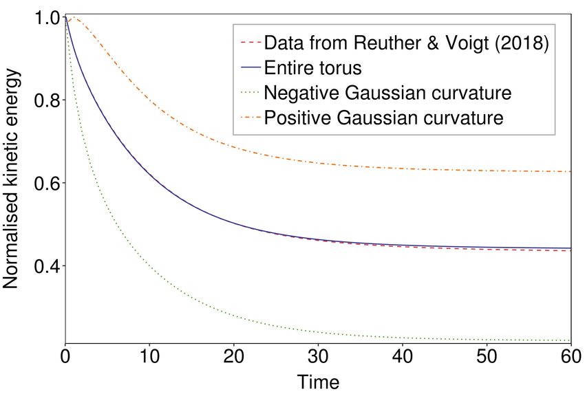
4                                 M. Rank and A. Voigt
with initial condition u(x, 0) = u0 (x) ∈ Tx M was proposed on M × (0, ∞) with M a
sphere. The tangential fluid velocity at point x ∈ M and time t ∈ (0, ∞) is denoted by
u(x, t) ∈ T M and the surface pressure by p(x, t) ∈ R. Mickelin et al. (2018) considers the
surface tension −p(x, t). ∂t is the time derivative, ∇u the covariant directional derivative,
gradM the surface gradient, and divM and divM the surface divergence, for vector- and
tensor-fields, respectively. The stress tensor T contains passive and active contributions
and reads

                                                                  T
                              T = f (∆M ) gradM u + (gradM u) ,                         (2.3)
                      f (∆M ) = Γ0 − Γ2 ∆M + Γ4 ∆2M ,                                   (2.4)
where ∆2M = ∆M ∆M with a surface Laplacian ∆M and real parameters Γ0 , Γ2 , Γ4 ∈ R.
The constants Γ0 and Γ4 are assumed to be positive to ensure asymptotic stability,
whereas Γ2 may have either sign. For Γ2 < 0 nontrivial steady-state flow structures
may emerge. Viewing f (∆M ) as an effective viscosity, sufficiently negative Γ2 may turn
this quantity negative and thus providing a source of energy which makes the model
effectively active. We can think about ∆M as a wildcard for any surface Laplacian.
Mickelin et al. (2018) have been using the Bochner Laplace operator ∆M = ∆B . Other
choices are the Laplace-deRham operator ∆dR or the Q-Laplacian ∆Q . They are related
by ∆Q u = ∆B u + κu = ∆dR u + 2κu, with κ the Gaussian curvature (Abraham et al.
2012). In flat space they are all identical and also for the sphere, where the Gaussian
curvature κ is constant, evaluating divM T is not an issue for any of the operators.
However, evaluating divM T on more general surfaces, like the torus, turns out to be
most convenient using the Q-Laplacian. This leads to the following computation:
                                                        T
        divM T = divM f (∆Q ) (gradM u + (gradM u) )
                = divM f (∆Q ) · 2∇Q u
                = 2Γ0 divM ∇Q u − 2Γ2 divM ∆Q ∇Q u + 2Γ4 divM ∆2Q ∇Q u
                = Γ0 · 2divM ∇Q u − Γ2 · 2divM ∇Q ∆Q u + Γ4 · 2divM ∇Q ∆2Q u
                = Γ0 ∆Q u − Γ2 ∆2Q u + Γ4 ∆3Q u,                                        (2.5)
where ∆3Q = ∆Q ∆Q ∆Q . Introducing the auxiliary quantities v = ∆Q u and w =
∆Q v = ∆2Q u, using eq. (2.5) and the Bochner Laplacian ∆B , eqs. (2.1) and (2.2) can
be rewritten as a system of second order partial differential equations
 ∂t u + ∇u u = −gradM p + Γ0 (∆B u + κu) − Γ2 (∆B v + κv) + Γ4 (∆B w + κw) , (2.6)
           v = ∆B u + κu,                                                               (2.7)
           w = ∆B v + κv,                                                               (2.8)
      divM u = 0,                                                                       (2.9)
which we will consider as a surface GNS equation on M , with M now a compact smooth
2-manifold without boundary. In the case of constant Gaussian curvature κ the model
coincides with the model presented in Mickelin et al. (2018) with the particular choice of
Γ0 = Γ0 − 2Γ2 κ + 4Γ4 κ2 , Γ2 = Γ2 − 4Γ4 κ and Γ4 = Γ4 . Thereby Γ0 , Γ2 and Γ4 denote the
according parameters introduced in Mickelin et al. (2018). For Γ2 = Γ4 = 0 we obtain as
a special case the surface NS equation (Scriven 1960). This limit, which also follows as
a thin-film limit of the 3D NS equation with Navier boundary conditions (Miura 2018;
Nitschke et al. 2019; Reuther et al. 2020) justifies the choice of the surface Laplacian in
the derivation. We further expect also to obtain eqs. (2.6)-(2.9) as a thin-film limit of the
3D GNS with Navier boundary conditions. However, this analysis has not been done.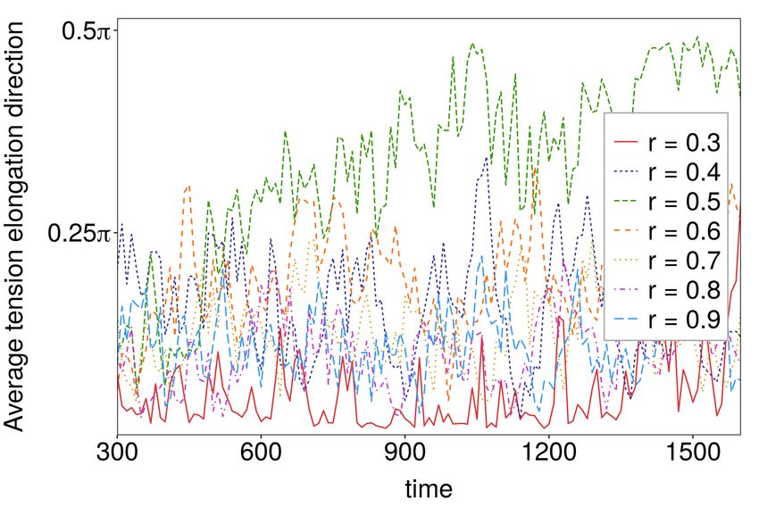
Active flows on curved surfaces                                  5
   It is not obvious to see why eqs. (2.6) - (2.9) provide an effective model for internally
driven flows. The active component is hidden in the effective viscosity f (∆Q ), which
accounts for the intrinsic solvent fluid viscosity and contributions representing the stresses
exerted by the active components on the fluid. For Γ2 < 0 an instability can occur and the
interplay between this instability and the nonlinerity of the surface NS equations drives
the spatiotemporal dynamics and leads in certain parameter regimes to the formation of
mesoscale vortices. Due to the additional coupling with geometric quantities we expect
the vortices and the parameter regime to be effected by the Gaussian curvature of the
surface. While for constant Gaussian curvature κ exact stationary solutions can be
constructed, which show some aspects of this influence (see Mickelin et al. 2018), for
the general case we have to rely on numerical approximations.

3. Numerical approach
   Following the general approach (Nestler et al. 2019) we first reformulate eqs. (2.6) -
(2.9) to a system which fulfils u(x, t) ∈ T M only approximately. This system can then
be numerically solved using a time discretisation based on a Chorin projection method
and a space discretisation by a regular surface triangulation and a scalar-valued surface
finite element method (Dziuk & Elliott 2013) applied to each component of the extended
velocity field, each component of the extended auxiliary variables and the pressure field.
The approach extends the surface finite element discretisation for the surface NS equation
(Reuther & Voigt 2018) to the surface GNS equation.

                                      3.1. Reformulation
   Instead of the tangential fields u(x, t), v(x, t), w(x, t) ∈ T M in the surface GNS
equation (2.6) - (2.9) we will consider R3 -valued vector fields û(x, t), v̂(x, t), ŵ(x, t) ∈ R3
which are only weakly tangential to T M . We thereby approximate the surface GNS
equation following the general method proposed by Nestler et al. (2019). We consider
a neighbourhood Uδ of M with coordinate projection π : Uδ → M of x̃ = a(x̃) +
d(x̃)ν (a(x̃)) ∈ Uδ , with d the signed distance function and ν the surface normal, given
by x̃ 7→ x = a(x̃) ∈ M . Depending on the curvature of the surface M , this coordinate
projection is injective for δ > 0 small enough. The velocity field, the auxiliary variables
and the pressure are smoothly extended to Uδ such that ũ(x̃) = u (x), ṽ(x̃) = v (x),
w̃(x̃) = w (x) and p̃(x̃) = p (x) are obtained for all x̃ ∈ Uδ . We extend the tangential
differential operators by
ˆ c û = π M · (∇û − ∇û · νν) ,
∇                                    c M û = div (û) − ν · (∇û · ν) ,
                                     div                                    ˆ B û = div
                                                                            ∆        dM ∇ˆ c û,

where ∇, div and div denote the common vector gradient and divergence operators
in R3 . For the general form for div
                                  d M we refer to Nestler et al. (2019)(Eq. E.2). The
pointwise normal projection is given by π M = I − νν T , where I denotes the identity
matrix. Adding α(ν · û)ν, α(ν · v̂)ν and α(ν · ŵ)ν with penalty parameter α ∈ R big
enough penalises the normal components of the vectors û, v̂ and ŵ, see Nestler et al.
(2019). This motivates the choice of the operators above, as we assume the velocity û
to be approximately tangential to the surface. In Nestler et al. (2019) it was shown
that ∆ˆ B û ≈ ∆B u, when using an appropriate penalty term. For convergence studies
and possible dependencies of α on mesh size, we refer to Hansbo et al. (2020). Reuther
& Voigt (2018) motivate the replacement of the surface divergence divM u by div c M û.
This leads to the following approximation of the surface GNS equation in Cartesian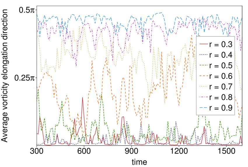
6                                    M. Rank and A. Voigt
coordinates:
                        ˆ c û = −∇
           ∂t û + û · ∇          ˆ c p + Γ0 v̂ − Γ2 ŵ + Γ4 (∆
                                                               ˆ B ŵ + κŵ) − α(ν · û)ν,   (3.1)
                                 ˆ B û + κû − α(ν · v̂)ν,
                            v̂ = ∆                                                           (3.2)
                               ˆ B v̂ + κv̂ − α(ν · ŵ)ν,
                          ŵ = ∆                                                             (3.3)
                   div
                   c M û = 0.                                                               (3.4)
The above model formulation coincides with the initial one just in the case of ν · û =
ν · v̂ = ν · ŵ = 0 and ensures only a weak form of tangency of the according solution û
(Reuther & Voigt 2018; Nestler et al. 2019). Hereafter, we assume the vector fields û, v̂,
and ŵ to be tangential to the surface, which is legitimate for appropriate α (Reuther &
Voigt 2018; Hansbo et al. 2020). Operators as well as functions will remain to have the
same nomenclature, although formally they differ. In particular, the ∧-sign of û, v̂, ŵ,
∇ˆ c , div
       c M and ∆ ˆ B will be omitted in the following.

                                     3.2. Time discretisation
  The procedure applied for the discretisation of time is based on Chorin (1968) and
Rannacher (1992) and was successfully applied by Reuther & Voigt (2018) for the surface
NS equation. For numerical reasons, we linearise the nonlinear covariant directional
derivative and obtain u∗ · ∇c u∗ ≈ un · ∇c u∗ . This yields the following problem with a
semi-implicit Euler time scheme:
  Let u0 := u0 ∈ T M be the sufficiently smooth initial velocity field and τn ∈ R be the
time step in the n-th iteration. For n → n + 1 determine successively
   (i) u∗ , v ∗ and w∗ such that
      1 ∗
        (u −un ) + (un ·∇c )u∗ − Γ0 v ∗ + Γ2 w∗ − Γ4 (∆B w∗ + κw∗ ) + α(ν · u∗ )ν = 0, (3.5)
     τn
                                                  v ∗ − ∆B u∗ − κu∗ + α(ν · v ∗ )ν = 0, (3.6)
                                                     w∗ − ∆B v ∗ − κv ∗ + α(ν · w∗ )ν = 0. (3.7)
    (ii) pn+1 such that
                                     τn ∆M pn+1 = divM u∗ ,                                  (3.8)
     with ∆M the Laplace-Beltrami operator.
    (iii) un+1 such that
                                    un+1 = u∗ − τn · ∇c pn+1 .                               (3.9)

                                   3.3. Space discretisation
                                      S
   A regular triangulation Mh = T ∈T T of the smooth surface M is constructed by
triangular elements T ∈ T determined by fixed points that are distributed equally over
the surface. Note that the particular choice of Mh in general also affects the normal
vector field. If analytically known, we define the unit normal vector field ν h of Mh as
the analytic normal of M in each degree of freedom (DOF). Otherwise, in order to
achieve convergence, an approximation is needed which is at least one order better than
the approximation of the surface (Hansbo et al. 2020). This can, e.g., be obtained by
locally reconstructing higher order approximations of Mh and computing the normals
from them, as, e.g., considered in Reuther et al. (2020); Nitschke et al. (2020a).
   The surface differential operators are manipulated to operate on Mh instead of M
essentially by using the pointwise normal projection onto Mh , which is given by π Mh =
I − ν h ν Th . We apply a scalar-valued surface finite element method for each component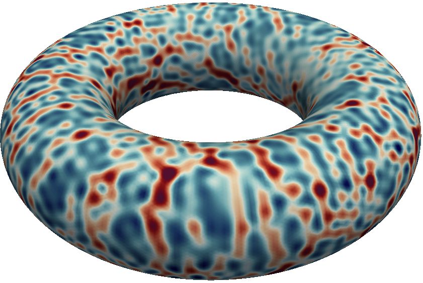
Active flows on curved surfaces                                               7
of the partial differential equations (Dziuk & Elliott 2013). The procedure is analogous
to the regular well-studied finite element method in flat space with the only difference
of a surface discretisation (Vey & Voigt 2007). The weak derivative, Sobolev spaces etc.
can bedefined in the same manner. We consider the piecewise linear finite element space
Vh = ϕ ∈ L2 (Mh ) : ϕ|T ∈ P1 for all T ∈ T for trial and test functions. For k = 1, 2, 3
let u∗k , vk∗ , wk∗ , unk , vkn and wkn be the sufficiently smooth k-th component of u∗ , v ∗ , w∗ ,
un , v n and wn , respectively. We multiply each component of equations (3.5)-(3.9) with
a smooth test function ϕ ∈ Vh , integrate over the domain Mh and apply the divergence
theorem to achieve the weak formulation. This yields the following time and space discrete
problem:
   Let u0 = u0k k with u0k ∈ Vh for all k = 1, 2, 3 be the initial velocity field. For n → n+1
determine successively
   (i) u∗k , vk∗ , wk∗ ∈ Vh such that
                            Z                   Z                          Z
                          1
                                  u∗k · ϕ dAh +     un ∇c u∗k · ϕ dAh − Γ0     vk∗ · ϕ dAh
                         τn Mh                   Mh                         Mh
                     Z                        Z                          Z
                              ∗                       ∗
             +Γ2            wk · ϕ dAh + Γ4       ∇c wk · ∇c ϕ dAh − Γ4      κwk∗ · ϕ dAh
                 Mh                           Mh                                      Mh
                                          3 Z                                        Z
                                          X                                      1
                                   +α                   νi u∗i νk · ϕ dAh =                 unk · ϕ dAh ,   (3.10)
                                          i=1      Mh                           τn     Mh

                 Z                        Z                               Z
                          vk∗ · ϕ dAh +            ∇c u∗k · ∇c ϕ dAh −             κu∗k · ϕ dAh
                     Mh                    Mh                               Mh
                                              3 Z
                                              X
                                     +α                    νi vi∗ νk · ϕ dAh = 0,                           (3.11)
                                              i=1     Mh

                 Z                        Z                                 Z
                          wk∗ · ϕ dAh +             ∇c vk∗ · ∇c ϕ dAh −              κvk∗ · ϕ dAh
                    Mh                        Mh                              Mh
                                              3 Z
                                              X
                                     +α                    νi wi∗ νk · ϕ dAh = 0                            (3.12)
                                              i=1     Mh

for every test function ϕ ∈ Vh and for all k = 1, 2, 3. Thereby, un = (unk )k with unk ∈ Vh
for all k = 1, 2, 3 denotes the solution from the previous time step n.
  (ii) pn+1 ∈ Vh such that
                       Z                         Z
                    τn     ∇c pn+1
                                    · ∇c ϕ dAh +     divM u∗ · ϕ dAh = 0              (3.13)
                           Mh                                  Mh

for every test function ϕ ∈ Vh .
  (iii) un+1
         k   ∈ Vh such that
             Z                   Z                                   Z
                   n+1
                                                u∗k                          ∇c pn+1 k · ϕ dAh .

                  uk · ϕ dAh =                        · ϕ dAh − τn                                          (3.14)
               Mh                         Mh                           Mh

for every test function ϕ ∈ Vh and for all k = 1, 2, 3.
The implementation of this algorithm is done with the help of the C++ based finite
element library AMDiS (see Vey & Voigt 2007; Witkowski et al. 2015) and the resulting
assembled linear systems are solved by BiCGSTAB(`) (Van der Vorst 1992).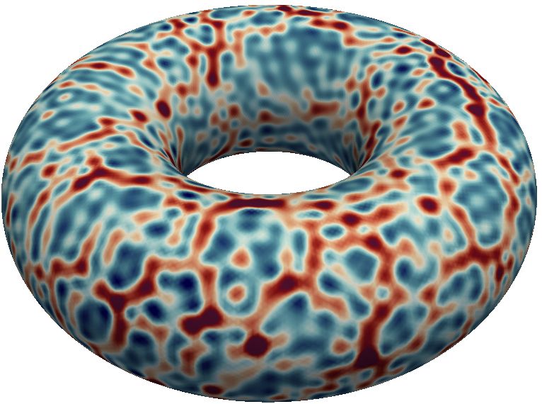
8 M. Rank and A. Voigt
Figure 1: Parameterisation of torus with inner and outer radius r and R = 1/r, and
corresponding angles θ1 and θ2 .
3.4. Validation
We validate the numerical approach against known results for passive flows on a torus
and active flows on a sphere. In the following, all presented numbers and values are
dimensionless quantities.
3.4.1. Passive flows on torus
We first consider passive flows on a torus. This has been done in detail by Reuther
& Voigt (2018), utilising a surface NS equation which is achieved by Γ0 = 1/Re and
Γ2 = Γ4 = 0. We consider the time step τn = 0.1 and the penalty parameter α = 3000.
The used mesh of the torus surface with outer radius R = 2.0 and inner radius r = 0.5
consists of 49.280 triangular elements and 24.640 vertices. To set the initial velocity field
u0 , we consider the arithmetic mean of the two linear independent harmonic vector fields,
1 1
uharm
θ1 = ∂θ x, uharm
θ2 = ∂θ x,
2kxk2 1 4kxk22 2
with θ1 , θ2 ∈ [0, 2π], see Figure 1 for a definition of the parameters. We normalise the
total kinetic energy of the system E(t) = 21 Mh ku(t)k2 dA by dividing by the maximum
R
value Emax = E(0) and compare it with the benchmark problem in Reuther & Voigt
(2018), see Figure 2(a). The agreement gives a first validation of the numerical approach.
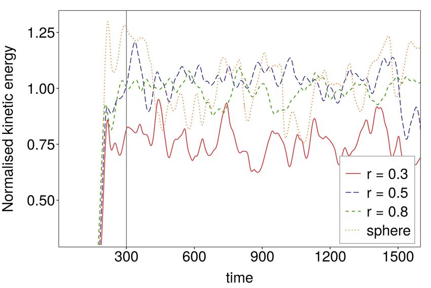
Figure 2(b) shows the normalised kinetic energy over time for different choices of the
inner radius r and according outer radius R = 1/r to preserve the surface area of the
torus. Already for this case a dependency of the dynamics on geometric properties is
realised. This includes not only a faster decay for increasing inner radius r, but also a
faster decay in regions of negative Gaussian curvature, see Figure 2(a).
3.4.2. Active flows on sphere
We next compare active flows on a sphere with results in Mickelin et al. (2018). We
consider parameters leading to anomalous vortex-network turbulence, compare case (d)
in Figure 2 of Mickelin et al. (2018). The penalty parameter α = 3, 000 is as in the passive
case, but the time step is reduced to τn = 0.005. As initial velocity field we consider a
random field. The sphere is discretised by 50,000 triangular elements and 25,002 vertices.
The radius of the sphere is R = 1. Figure 3(a) shows a snapshot of the normalised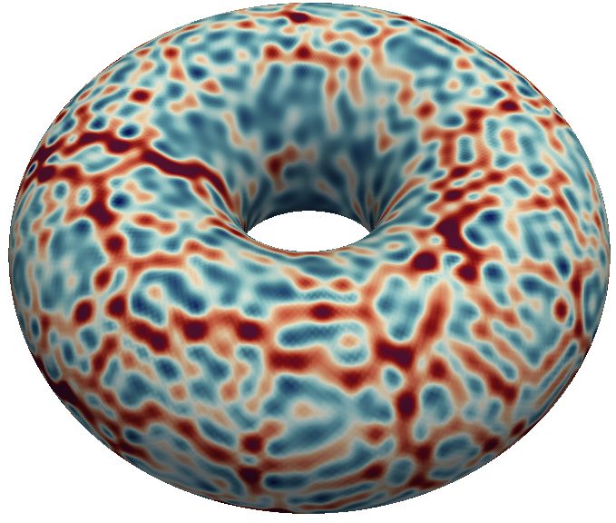
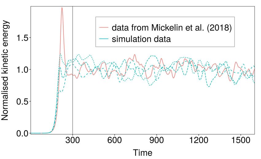
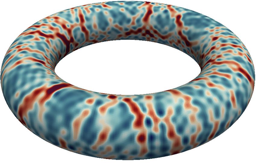
Active flows on curved surfaces                             9
(a)                                             (b)

Figure 2: Normalised total kinetic energy of the implemented model with parameters
Γ0 = 0.1 and Γ2 , Γ4 = 0, penalty parameter α = 3000, time step τn = 0.1 and (a) torus
radii r = 0.5 and R = 2.0 and the results from Reuther & Voigt (2018) (dashed line),
on the entire surface and on regions of positive and negative Gaussian curvature, and
(b) different choices of radii r = 0.3, 0.4, ..., 0.9, with R = 1/r accordingly, on the entire
domain, against time. The distinction between regions of positive and negative Gaussian
curvature for different r leads to the same behaviour as shown in (a).

(a)                       (b)                         (c)

(d)

Figure 3: Snapshots of (a) vorticity and (b) surface tension field at time t = 860. (c)
Normalised kinetic energy - total kinetic energy divided by mean kinetic energy after
relaxation, indicated by vertical grey line at t = 300 - against time in comparison with
data from Mickelin et al. (2018). Considered parameters are Γ0 = 3.901565 · 10−2 , Γ2 =
−7.886719 ·10−5 and Γ4 = 3.887· 10−8 . Different line types emerge from different random
initial conditions. (d) Distribution of frequencies found by FFT averaged over three
simulation runs, the strength is given by the absolute value of the according coefficient
of the FFT. Black lines indicate the according sample standard deviation.

vorticity field. The vorticity is computed by φ = curlM u, with curlM the surface rotation,
defined by curlM u = divM (u × ν) and u to be interpreted as the tangential velocity
field supplemented with a third component in normal direction set to be zero. φ is
a scalar field, the magnitude of the vector pointing in normal direction. Figure 3(b)
shows the corresponding normalised surface pressure/surface tension. To be comparable
the considered normalisation follows Mickelin et al. (2018). Anomalous vortex-network
turbulence is characterised in Mickelin et al. (2018) by topological measures of the
10                                M. Rank and A. Voigt

Figure 4: Convergence properties for vorticity, pressure/tension and kinetic energy. The
L2 error is computed with respect to the solution on the finest mesh and shown with
respect to the number of degrees of freedom (DoFs). The black and the red lines indicate
order 1 and 1/2, respectively.

vorticity and geometric measures of the high-tension domains. The last shows highly
branched chain-like structures which are clearly visible in Figure 3(b). This provides a
further qualitative validation of the numerical approach. Finite-size vortices self-organise
into chain complexes of antiferromagnetic order that percolate trough the entire surface
forming an active dynamic network, which provides an efficient mechanism for upward
energy transport from smaller to larger scales. The dynamics of this process is validated
against Mickelin et al. (2018) in Figure 3(c) by comparing the normalised kinetic energy,
the total kinetic energy divided by the mean kinetic energy after relaxation. As the initial
data in Mickelin et al. (2018) is not known, we consider different simulations with different
initial data. The relaxation time, as well as the amplitude and frequency of the observed
oscillations are independent on the initial data and in reasonable agreement with Mickelin
et al. (2018). To compare the amplitudes of the energy curves, we have computed the root
                            1
                                R T2           2    1
mean square RMS = ( T2 −T     1   T1
                                      E(t) − Ē dt) 2 with T1 = 300 and T2 = 1600, and
mean kinetic energy Ē. The computed values are RMS = 0.129, 0.109 and 0.070 for our
simulations and RMS = 0.087 for the data of Mickelin et al. (2018) with peak-to-peak
amplitude values of 0.487, 0.486, 0.333 and 0.415, respectively. A Fast Fourier Transform
(FFT) gives the dominant frequencies, see Figure 3(d). Quantitative differences result
from different initial conditions but probably also from different approximations of
geometric quantities. Other measures, such as size of vortices and high-tension domains
are in agreement and qualitatively, our simulations are within the anomalous vortex-
network turbulence regime identified in Mickelin et al. (2018).
   To demonstrate the appropriate choice of the numerical parameters we consider differ-
ent mesh resolutions. Mesh refinement is done by bisection with new vertices projected to
the spherical surface. To circumvent relaxation effects in the initialisation phase we start
with initial conditions, obtained from the previous simulations after t = 300, which are
interpolated to the new meshes. The solutions are almost indistinguishable by eye from
the one plotted in Figure 3(a) and (b). Figure 4 shows the L2 -errors in the vorticity φ and
surface pressure / surface tension p, as well es differences in the kinetic energy E after
400 time steps with constant time step τn . The mesh used for the simulations shown in
Figure 3(a) and (b) corresponds to the second data point in Figure 4. The results indicate
convergence of order 1/2 with respect to the number of degrees of freedom (DoFs) for
the vorticity. This relates to order 1 with respect to mesh size. Surface pressure / surface
tension and kinetic energy show convergence of order 1 with respect to number of DoFs
and order 2 with respect to mesh size.
   These results for the full model on a sphere together with the results of the surface NS
Active flows on curved surfaces 11
equation on a torus make the proposed numerical scheme trustworthy to be applied for
the full model on toroidal surfaces, in oder to explore the influence of local variations in
Gaussian curvature on the anomalous turbulence regime.
4. Results
4.1. Measures for topological and geometric quantities
In analogy to Mickelin et al. (2018) we determine the topology of the vorticity fields
and the geometry of the high-tension domains to identify anomalous turbulence. We
therefore define the normalised Betti number as
hNφ (r, t) − Nsphere (t)i
Bettiφ (r) = ,
hNsphere (t)i
with Nsphere (t) denoting the zeroth Betti number of a sphere with radius R = 1 at time
t as a reference value. The zeroth Betti number Nφ (r, t), with r the inner radius of
the considered torus, measures the number of connected domains with a high absolute
vorticity {x ∈ M : φ(x, t) > αφ · maxx∈M φ(x, t) or φ(x, t) < αφ · minx∈M φ(x, t)} and
a threshold αφ > 0 at time t. The time average h·i is taken after the initial relaxation
period. Intuitively, large values of Bettiφ indicate many vortices of comparable circulation
or many connected structures of similar size, whereas small values suggest the presence of
a few dominant eddies or large connected structures. Accordingly, the normalised Branch
number is defined by
hAp (r, t) − Asphere (t)i
Branchp (r) = ,
hAsphere (t)i
with Asphere (t) serving as a reference value. The Branch number Ap (r, t) denotes the mean
of the ratios ∂A/A, where A denotes the area and ∂A denotes the boundary length of
each connected component of the regions {x ∈ M : p(x, t) > βp p̄(t)} with p̄ its mean
value and βp > 0 a parameter. The ratio ∂A/A is a measure of chainlike structures
in the surface pressure/surface tension fields, a large value signaling a highly branched
structure, whereas smaller values indicate less branching. Nsphere (t) and Asphere (t) are
considered to compare with anomalous turbulence in the spherical case in Mickelin et al.
(2018).
4.2. Active flows on toroidal surface
We are using a mesh with 48,832 vertices and 97,664 resulting triangle elements, which
we scale to approximate all tori with inner radius r and according outer radius R = 1/r.
The total simulation time is T = 1600, which turns out to be sufficient to reveal the
characteristic active dynamics of the system.
The separation of the general model dynamics into a relaxation phase and an active
chaotic phase can be done in the same way as already described for the sphere with gener-
ating and dissolving similar vortex patterns for all choices of inner radii r. Figure 5(a),(b)
show snapshots of the normalised vorticity and the nomalised surface pressure/surface
tension of a simulation on a torus. As for the sphere, the relaxation phase also runs
until about t = 300. Thereafter the active regime begins. Comparing the still images
of the torus and the sphere, the vorticity seems to have the tendency to form slightly
more complex, longer and maze-like structures on the torus. The tension still has the
characteristic branched chain-like structures. However, the images give an impression on
prefered orientations of the structure. Nevertheless, the patterns and dynamics appear
to be qualitatively similar to the ones on a sphere. To investigate the differences between12 M. Rank and A. Voigt
(a) (b) (c)
(d)
Figure 5: Snapshots of (a) vorticity and (b) surface tension field on torus with radii
r = 0.5 and R = 2.0. Other parameters are as in Figure 3. (c) Normalised kinetic energy
- total kinetic energy for different choices of radii r = 0.3, 0.5, 0.8 with R = 1/r divided
by average total kinetic energy over all tori after relaxation - against time. The vertical
grey line at t = 300 marks the beginning of the active turbulence regime. The results
for a sphere are shown for comparison. (d) Distribution of frequencies found by FFT,
averaged over three simulation runs, the strength is given by the mean absolute value of
the according coefficient of the FFT. Black lines indicate the according sample standard
deviation.
Inner radius r 0.3 0.4 0.5 0.6 0.7 0.8 0.9 sphere
Average normalised kinetic energy 0.761 0.855 1.032 1.080 1.059 0.992 0.931 1.017
Peak-to-peak amplitude 0.494 0.316 0.347 0.220 0.227 0.222 0.260 0.504
RMS value 0.093 0.061 0.067 0.044 0.041 0.052 0.051 0.128
Table 1: Average normalised kinetic energy, see Figure 5(c), peak-to-peak amplitude and
root mean square (RMS) values of normalised kinetic energy curves, averaged over time
and simulation runs for tori with inner radius r and sphere with R = 1.
the simulation results on the sphere and the toroidal surfaces for different radii r and
R = 1/r we compute the normalised kinetic energy, see Figure 5(c), and the average
RMS values over three simulation runs, see Table 1. The kinetic energy progressions
of the different tori are similar to each other and to the sphere. Nevertheless, thin tori
with inner radius r = 0.3, 0.4 appear to have larger energy fluctuations than thick tori
with r = 0.8, 0.9. This observation is underlined by the peak-to-peak amplitude values.
The distribution of frequencies in the FFT of the tori is shown in Figure 5(d). We can
detect similar dominant frequencies for all tori with no significant differences between the
various torus dimensions. Depending on the random initial conditions, distinct frequency
distributions emerge, see Figure 5(d).
To explain the observed differences in the energy fluctuations requires a deeper analysis
of the data. The normalised Betti and Branch numbers for the whole surface have been
computed for tori with inner radius r = 0.3, 0.4, ..., 0.9 and according outer radiusActive flows on curved surfaces 13
Inner radius r 0.3 0.4 0.5 0.6 0.7 0.8 0.9
Bettiφ (r) per area -0.436 -0.161 -0.166 -0.067 -0.055 -0.182 -0.568
Branchp (r) per area 2.438 1.555 1.291 1.563 1.673 0.820 0.733
Table 2: Normalised Betti and Branch numbers per area for the entire surface averaged
over simulation runs for tori with inner radius r.
(a) (b) (c) (d)
Figure 6: Gaussian curvature κ from blue to red on tori with inner radius a) r = 0.3,
b) r = 0.5, c) r = 0.7, d) r = 0.9 and according outer radius R = 1/r. r does not scale
between (a) - (d).
R = 1/r with parameters αφ = 0.5 and βp = 1. They are divided by area and their
averaged values, over different simulation runs, are given in Table 2. We can observe
lower normalised Betti numbers for very thin (r = 0.3) and very thick (r = 0.9) tori.
The normalised Branch numbers show a different trend. They are largest for very thin
(r = 0.3) and smallest for thick (r = 0.8, 0.9) tori.
However, averaging over the entire surface does not account for the local differences in
surface curvature. To extract a dependency of the normalised Betti and Branch numbers
on local curvature we classify regions of equal Gaussian curvature on all considered
tori. Figure 6 shows the different values of Gaussian curvature κ on selected tori. While
moderate values of positive Gaussian curvature are found on the outer part for all tori,
strong negative values are only present in the inner part of thick tori (r = 0.8, 0.9).
We visualise the normalised Betti and Branch numbers per area for the different
tori according to intervals of Gaussian curvature, see Figure 7. This indicates a clear
dependency of the normalised Betti number on the Gaussian curvature, with a maximal
value for Gaussian curvature between −1 and 0 and decreasing values for lower and higher
Gaussian curvatures. Moderate values of Gaussian curvature show a similar behaviour
as in the spherical case and thus indicate anomalous turbulence, whereas larger absolute
values favour the presence of fewer more dominant vortices and thus deviation from the
anomalous turbulence regime, see Mickelin et al. (2018). The behaviour for the normalised
Branch number is similar, with maximal values for Gaussian curvature between −1.5 and
0 and decreasing values for lower and higher Gaussian curvatures. While this is true for
all tori, the values between the different tori strongly differ. They are largest for very
thin tori (r = 0.3) and decrease towards very thick tori (r = 0.9). For all regions the
normalised Branch number is larger than in the representative spherical case, indicating
even enhance branching. The movies in the Electronic Supplement confirm this and show
the characteristic percolation of the high tension structures through the entire domain.
A characterisation of the flow regime as anomalous turbulence requires the topology of
the vorticity fields and the geometry of the high-tension domains to be characteristic
(Mickelin et al. 2018). Both together thus indicate anomalous turbulence for moderate
regions of Gaussian curvature, and possible deviations for lower and higher values. We14 M. Rank and A. Voigt
(a) (b)
(c) (d)
Figure 7: a) Normalised Betti numbers per area for surface areas with Gaussian curvature
(κ − 0.1, κ + 0.1), κ ∈ {−2.4, −2.2, ..., 0.8} and b) normalised Branch number for surface
areas with Gaussian curvature (κ − 0.25, κ + 0.25), κ ∈ {−2.25, −1.75, ..., 0.25} vs. inner
torus radius r, the row at the bottom showing the average value over all considered
torus geometries. A few intervals of Gaussian curvature are not found on some tori,
indicated by grey colour, see Figure 6. The average values with according sample standard
deviation of different simulation runs are shown in c) for the normalised Betti number
and values for one simulation in d) for the normalised Branch number. The black lines
show the according mean values over all runs and tori. The results are obtained with
the parameters αφ = 0.5 and βp = 1. Results for different parameters are shown in the
Appendix and demonstrate the robustness of the results.
also compute the enstrophy E(t) = Mh φ2 dA for the whole surface and per region of
R
constant Gaussian curvature, see Figure 8(a) and (b), respectively. The values are largest
for moderate tori (r = 0.5, 0.6, 0.7) and decay towards thinner (r = 0.3, 0.4) and thicker
(r = 0.8, 0.9) tori, see also Table 3. In Mickelin et al. (2018) it is argued that also the
ratio between the mean kinetic energy and the mean enstrophy can be used to identify
the anomalous turbulence regime. Even if this can only be a qualitative measure the
ratio is shown in Table 3. It shows a minimum for moderate tori (r = 0.5, 0.6, 0.7) and
moderate Gaussian curvature values (κ ∈ [−1.5, 0.0]), for which anomalous turbulence is
already identified and only slightly increases for thinner and thicker tori and lower and
higher Gaussian curvature values, respectively. This weak indication on the influence of
curvature effects on the active turbulence regime is consistent with the topological and
geometric measures of the normalized Betti and Branch numbers.
For all considered measures we see a dependency on the global shape of the torus.
However, the normalised Betti and Branch numbers, but also the nomalised enstrophy,
indicate that the flow regime of anomalous turbulence depends also on the local geometry.
Similar dependencies on local curvature have been found for topological defects in active
nematic toroids (Ellis et al. 2018). These results are in contrast to equilibrium systems,Active flows on curved surfaces 15
(a) (b)
Figure 8: a) Enstrophy per surface area nomalised by mean after relaxation over all tori,
shown for inner torus radius r = 0.3, . . . , 0.9. (b) Normalised enstrophy for surface areas
with Gaussian curvature (κ − 0.25, κ + 0.25), κ ∈ {−2.25, −1.75, ..., 0.25} vs. inner torus
radius r, the row at the bottom showing the average value over all considered torus
geometries.
Inner radius r 0.3 0.4 0.5 0.6 0.7 0.8 0.9
Normalised enstrophy per area 0.632 0.893 1.138 1.195 1.142 1.049 0.954
hE(t)i/hE(t)i 1.257 0.999 0.946 0.942 0.967 0.987 1.019
Gaussian curvature κ -2.25 -1.75 -1.25 -0.75 -0.25 0.25
hE(t)i/hE(t)i 1.089 1.078 0.881 0.967 0.974 1.034
Table 3: Mean normalised enstrophy per area over time and simulation runs for tori
with inner radius r. Ratio of mean normalized kinetic energy and mean normalized
enstrophy per area for tori with inner radius r as well as intervals of Gaussian curvature
(κ − 0.25, κ + 0.25).
which predict only a dependency on the global parameters r and R (see Bowick et al.
2004; Giomi & Bowick 2008; Jesenek et al. 2015). We will further elaborate on the relation
to the experiments in Ellis et al. (2018) below.
We first address an observation in the movies in the Electronic Supplement. They
indicate a preferred direction of the chained vortex structures. They seem to align with
the principle curvature lines and prefer the one with lower absolute value of Gaussian
curvature. For regions of positive Gaussian curvature (outer part) they align horizontally,
whereas for negative Gaussian curvature (inner part), at least for strong values, the
alignment is vertically. This observation is confirmed in Figure 9(b) showing the average
direction of elongation of the chained vortex structures. The still image in Figure 9(a) can
only partly confirm this, we therefore refer to the corresponding movies in the Electronic
Supplement. Figure 9(d) and (c), show the corresponding average direction of elongation
of high-tension domains and a characteristic still image, respectively. Representative
still images for the other radii are provided in the Appendix. The average directions
have been computed using a method first introduced for quantifying deformations of
foam structures by Asipauskas et al. (2003) and was later applied for the elongation
of cellular structures (Mueller et al. 2019). To apply it for our situation we represent
the geometry of the chained vortex structures and the branched high-tension field as
phase fields, i.e. scalar fields that take values one on the inside and zero on the outside of16 M. Rank and A. Voigt
Inner radius r 0.3 0.4 0.5 0.6 0.7 0.8 0.9
Vorticity elongation eigenvalue 0.086 0.081 0.066 0.053 0.051 0.068 0.083
Table 4: Elongation eigenvalue averaged over time and simulation runs for tori with inner
radius r.
the segmented structures with a smooth transition over a small interface. All information
about the elongation can be represented in terms of the gradient of these phase fields. The
elongation is described as the angle against the lines of constant Gaussian curvature, i.e.
the green lines in Figure 1. Thus, an elongation of zero represents a horizontal structure
aligned with the green lines and a values of π/2 represents a vertical structure aligned
with the red lines of Figure 1. As we solely want to determine the elongation of large
structures, we only consider areas that are bigger than the 99% quantile of all areas. At
least for thin tori (r = 0.3, 0.4) and thick tori (r = 0.8, 0.9) this preferred alignment of
the chained vortex structures becomes evident. The elongation of the tension fields is less
evident. Only for thin tori (r = 0.3, 0.4) a preferred horizontal elongation is observed. A
preferred vertical elongation for thick tori (r = 0.8, 0.9) can not be seen. This might result
from less dominant branched structures in regions of strong negative Gaussian curvature,
see Figure 7(b),(d). For moderate tori (r = 0.5, 0.6, 0.7) the average elongation direction
of the tension fields fluctuates much stronger with no preferred orientation. Similar
alignment effects with minimal curvature lines have also been reported for surface liquid
crystals (Segatti et al. 2016; Nestler et al. 2018, 2020; Pearce 2020), at least if extrinsic
curvature effects are taken into account in the surface models (Nestler et al. 2020; Pearce
2020).
Besides this alignment effect with minimal curvature lines the deformation of the vortex
structures is also affected by the geometry of the tori. For the chained vortex structures
the according mean elongation eigenvalues over all structures of the computations are
shown in Table 4. It represents the mean deformation of the structures, lower values
indicating more circular patterns. The values are largest for more extreme cases, thin tori
(r = 0.3, 0.4) and thick tori (r = 0.8, 0.9), and lowest for moderate tori (r = 0.5, 0.6, 0.7).
While the previous results mainly indicate a general dependency on the absolute
value of the Gaussian curvature, there are also indications on a dependency on the sign
of the Gaussian curvature. The only available experimental results for active systems
on toroidal surfaces (Ellis et al. 2018) clearly show a dependency on the sign. The
corresponding simulations (Pearce et al. 2019), with the limitations discussed in the
introduction, qualitatively show a higher density of vortices in the interior of the torus. In
the considered active nematic system this is quantified by the topological charge density,
defect creation and annihilation rates, which are shown to depend approximately linearly
on Gaussian curvature. The GNS equation is a minimal phenomenological model, unable
to resolve these details. However, we can measure the number of vortices per area. Figure
10(a) shows the normalised Betti number per area for positive and negative Gaussian
curvature regions for all considered tori. With the exception for thick tori (r = 0.8, 0.9)
we observe the same behaviour, the number of vortices in the interior of the tori is higher.
This confirms a dependency also on the sign of the Gaussian curvature. The discrepancy
for thick tori (r = 0.8, 0.9) results from the different magnitudes of the vorticity regions
that are counted by the Betti number. Figure 10(b) shows the average total kinetic energy
for different regions of the tori. We can observe significantly lower values for regions of
strong negative Gaussian curvature. This results in lower normalised Betti numbers forActive flows on curved surfaces 17
(a) (b)
(c) (d)
Figure 9: Average direction of elongation of chained vorticity (b) and branched high-
tension structures (b) on different tori over time. The elongation direction is considered
with respect to the parameterisation. Snapshots of the considered vorticity and surface
tension structures for a torus with inner radius r = 0.8 are shown in (a) and (c),
respectively. For still images of the other tori see Appendix.
(a) (b)
Figure 10: (a) Normalised Betti numbers per area vs. inner torus radius for surface areas
with positive and negative Gaussian curvature obtained with parameter αφ = 0.5. Dotted
lines show the means over all tori and dashed lines show the according means over all tori
with r ∈ {0.3, 0.4, 0.5, 0.6, 0.7}. (b) Average total kinetic energy for surface areas with
Gaussian curvature (κ − 0.1, κ + 0.1), κ ∈ {−2.8, −2.6, ..., 0.8} divided by overall mean
total kinetic energy of each torus.18 M. Rank and A. Voigt thick tori (r = 0.8, 0.9), as more vorticies fall below the considered threshold. Figure 10(a) also shows the average values over all tori, with and without the two thick tori (r = 0.8, 0.9). Lower kinetic energy for regions with negative Gaussian curvature and higher values for regions with positive Gaussian curvature can already be seen for the surface NS equation in Figure 2. The effect probably results form the +Γ0 κu term in eq. (2.6), which, if neglecting all other contributions, leads to exponential decay for κ < 0 and exponential growth for κ > 0. It has to remain speculative if this simple explanation can also be used for the highly nonlinear surface GNS equation. Another interesting aspect of Figure 10(b) are the values at κ = 0. The differences for different tori indicate not only a dependency on the local Gaussian curvature but also on its gradient, which is largest for thin tori r = 0.3 and decreases with increasing r. Again this behaviour is in accordance to the experiments in Ellis et al. (2018). 5. Conclusions We consider a surface generalised Navier-Stokes (GNS) equation as a minimal model for active flows on arbitrarily curved surfaces. This extends work of Mickelin et al. (2018), who considered this equation on a sphere. The numerical approach extends work of Reuther & Voigt (2018) for the surface Navier-Stokes (NS) equation and is based on the general concept to solve surface vector-valued partial differential equations on arbitrary surfaces by surface finite elements (Nestler et al. 2019). We focus on toroidal surfaces, as a prototypical example of surfaces with varying Gaussian curvature with positive and negative values and consider parameter settings which lead to anomalous chained turbulence on a sphere (Mickelin et al. 2018). We here concentrate on the influence of Gaussian curvature on this new regime of active turbulence. The simulation results suggest that this turbulence regime can be influenced by global properties of the surface but also via the local Gaussian curvature and its gradients. The chained vortex structures have the tendency to align with minimal curvature lines of the surface. At the outer part (positive Gaussian curvature) they show a tendency to align horizontally and at the inner part (negative Gaussian curvature) they seem to align vertically, at least for thick tori. The considered topological and geometrical measures for the vorticity and high-tension fields, the normalised Betti and Branch numbers, indicate anomalous turbulence for moderate values of Gaussian curvature and possible deviations for lower and higher values. Also the kinetic energy and the enstrophy not only depend on the global properties of the torus but also on the local Gaussian curvature. Their ratio, another, at least qualitative, measure for anomalous turbulence (Mickelin et al. 2018) only slightly deviates for more extreme values for the inner radius r or the local Gaussian curvature κ, and shows the same weak dependency on curvature as the considered topological and geometric measures. While a full understanding of the relation of Gaussian curvature on active turbulence requires many further investigations, the simulations results indicate a clear dependency of various aspects on the Gaussian curvature of the surface. Some are in qualitative accordance with the experiments on active nematic liquid crystals, which are constrained to lie on a toroidal surface, see Ellis et al. (2018). These are larger numbers of vortices in regions of negative Gaussian curvature and a dependency on the gradient in Gaussian curvature on the kinetic energy. Other effects, such as the alignment of the chained structures with minimal curvature lines, ask for experimental validation. Another interesting question for future research is the influence of local Gaussian curvature on the transitions to classical 2D Kolmogorov turbulence. This transition is addressed in flat space and on the sphere (see Bratanov et al. 2015; James et al. 2018; Mickelin et al.
Active flows on curved surfaces                          19
(a)               αφ = 0.4                    (b)                αφ = 0.5

(c)               αφ = 0.6                    (d)               αφ = 0.75

Figure 11: Normalised Betti numbers per area as in Figure 7(a) for different
thresholds to define regions with high absolute vorticity {x ∈ M : φ(x, t) > αφ ·
maxx∈M φ(x, t) or φ(x, t) < αφ · minx∈M φ(x, t)}, with (a) αφ = 0.4, (b) αφ = 0.5,
(c) αφ = 0.6 and (d) αφ = 0.75.

2018; Linkmann et al. 2019, 2020b,a).

  Acknowledgment: This research was supported by the German Research Foundation
(DFG) within the Research Unit 3013. We used computing resources provided by ZIH at
TU Dresden and by Jülich Supercomputing Centre within project HDR06. We further
acknowledge the provided data from Mickelin et al. (2018) by O. Mickelin and J. Dunkel,
as well as support from M. Nestler, M. Salvalaglio and D. Wenzel concerning the
postprocessing.

Appendix A.
  Figures 11 and 12 provide the same information as Figure 10 for different thresholds
αφ and βp , demonstrating the robustness of the results on these values. Figure 13 and
14 show the corresponding still images for the vorticity and tension structures in Figure
9 for the other tori. For the corresponding videos and additional visualizations of the
surface velocity using LIC we refer to the Electronic Supplement.

                                    REFERENCES
Abraham, R., Marsden, J.E. & Ratiu, T. 2012 Manifolds, Tensor Analysis, and
     Applications. Springer New York.
Alaimo, F., Koehler, C. & Voigt, A. 2017 Curvature controlled defect dynamics in
     topological active nematics. Sci. Rep. 7, 5211.
20 M. Rank and A. Voigt
(a) βp = 0.8 (b) βp = 0.9
(c) βp = 1.1 (d) βp = 1.2
Figure 12: Normalised Branch numbers per area as in Figure 7(b) for different regions
{x ∈ M : p(x, t) > βp · p̄(t)} with (a) βp = 0.8, (b) βp = 0.9, (c) βp = 1.1 and (d)
βp a = 1.2.
(a) r = 0.3 (b) r = 0.4 (c) r = 0.5 (d) r = 0.6
(e) r = 0.7 (f) r = 0.8 (g) r = 0.9
Figure 13: Snapshots of normalised vorticity fields on different torus surfaces in the active
regime.
Apaza, L. & Sandoval, M. 2018 Active matter on Riemannian manifolds. Soft Matter 14,
9928–9936.
Asipauskas, M., Aubouy, M., Glazier, J., Graner, F. & Jiang, Y. 2003 A texture tensor to
quantify deformations: The example of two-dimensional flowing foams. Granular Matter
5, 71–74.
Beresnev, I.A. & Nikolaevskiy, V.N. 1993 A model for nonlinear seismic-waves in a medium
with instability. Physica D 66, 1–6.You can also read