Spatiotemporal Downscaling of GRACE Total Water Storage Using Land Surface Model Outputs
←
→
Page content transcription
If your browser does not render page correctly, please read the page content below
remote sensing
Article
Spatiotemporal Downscaling of GRACE Total Water Storage
Using Land Surface Model Outputs
Detang Zhong * , Shusen Wang                      and Junhua Li

                                          Canada Center for Remote Sensing, Canada Centre for Mapping and Earth Observation, Natural Resources
                                          Canada, 560 Rochester Street, Ottawa ON K1A 0E4, Canada; shusen.wang@canada.ca (S.W.);
                                          junhua.li@canada.ca (J.L.)
                                          * Correspondence: detang.zhong@canada.ca; Tel.: +1-613-759-6192

                                          Abstract: High spatiotemporal resolution of terrestrial total water storage plays a key role in assessing
                                          trends and availability of water resources. This study presents a two-step method for downscaling
                                          GRACE-derived total water storage anomaly (GRACE TWSA) from its original coarse spatiotemporal
                                          resolution (monthly, 3-degree spherical cap/~300 km) to a high resolution (daily, 5 km) through
                                          combining land surface model (LSM) simulated high spatiotemporal resolution terrestrial water
                                          storage anomaly (LSM TWSA). In the first step, an iterative adjustment method based on the self-
                                          calibration variance-component model (SCVCM) is used to spatially downscale the monthly GRACE
                                          TWSA to the high spatial resolution of the LSM TWSA. In the second step, the spatially downscaled
                                          monthly GRACE TWSA is further downscaled to the daily temporal resolution. By applying the
                                          method to downscale the coarse resolution GRACE TWSA from the Jet Propulsion Laboratory
                                          (JPL) mascon solution with the daily high spatial resolution (5 km) LSM TWSA from the Ecological

                                          Assimilation of Land and Climate Observations (EALCO) model, we evaluated the benefit and
                                   effectiveness of the proposed method. The results show that the proposed method is capable to
Citation: Zhong, D.; Wang, S.; Li, J.     downscale GRACE TWSA spatiotemporally with reduced uncertainty. The downscaled GRACE
Spatiotemporal Downscaling of             TWSA are also evaluated through in-situ groundwater monitoring well observations and the results
GRACE Total Water Storage Using           show a certain level agreement between the estimated and observed trends.
Land Surface Model Outputs. Remote
Sens. 2021, 13, 900. https://doi.org/     Keywords: land surface model; GRACE; EALCO; SCVCM; total water storage; downscaling
10.3390/rs13050900

Academic Editors: Augusto Getirana,
Sujay Kumar and Benjamin Zaitchik         1. Introduction
                                               Accurate knowledge on total or terrestrial water storage (TWS) and its spatiotemporal
Received: 26 January 2021
Accepted: 23 February 2021
                                          variability play a crucial role in the assessment of climate variation and water resource
Published: 27 February 2021
                                          availability [1]. The accuracy of TWS simulated by land surface models (LSMs) at high
                                          spatial and temporal resolution is commonly limited by uncertainties in meteorological
Publisher’s Note: MDPI stays neutral
                                          forcing, model parameter calibration, and land surface process representation [2–5]. To
with regard to jurisdictional claims in
                                          reduce the model uncertainties, researchers have been developing new LSMs that may
published maps and institutional affil-   account for interactions among the different components (e.g., soil moisture, groundwater,
iations.                                  surface water, and snow) of TWS. For instance, some models introduced the impact of
                                          groundwater on surface processes [6–9] and others added surface runoff algorithms based
                                          on empirical relationships [6,10,11]. Including groundwater in an LSM enables a more
                                          complete simulation of the terrestrial water cycle, but it is also subject to large uncertainties
Copyright: © 2021 by the authors.
                                          since the hydrogeological conditions of aquifers are largely unknown in many circum-
Licensee MDPI, Basel, Switzerland.
                                          stances. Due to differences in model physics and parameter values, estimates from various
This article is an open access article
                                          LSMs often exhibit large discrepancies even when models are run using identical forcing
distributed under the terms and           data [12–15]. These discrepancies impose large limitations in many hydrological applica-
conditions of the Creative Commons        tions and assessments. To improve quality of the TWS simulated by LSMs, researchers
Attribution (CC BY) license (https://     have been developing new models and algorithms that can combine or assimilate the
creativecommons.org/licenses/by/          temporal water storage changes or anomalies detected by the joint NASA/DLR Gravity
4.0/).                                    Recovery and Climate Experiment (GRACE) satellite [16] and its follow-on missions. Since

Remote Sens. 2021, 13, 900. https://doi.org/10.3390/rs13050900                                      https://www.mdpi.com/journal/remotesensing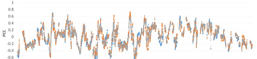
Remote Sens. 2021, 13, 900                                                                                       2 of 19

                             the GRACE system provides the only observation of the Earth’s TWS which includes all
                             water storage components, e.g., snow mass, surface water, vegetation water, soil moisture,
                             and groundwater [16], it gives us a valuable calibration to the LSM TWS outputs. At the
                             same time, we can also use it to improve LSM TWS accessibility through combination of
                             both datasets.
                                  Since the launch of the GRACE satellite in 2002, many researchers have been devel-
                             oping new models and algorithms for combining or assimilating GRACE observations
                             and LSM TWS outputs. For example, Zaitchik et al. [17] developed an ensemble Kalman
                             smoother (EnKS) to assimilate GRACE TWS into the NASA Catchment model in the Mis-
                             sissippi basin with promising results in 2008. Since then, different applications based on
                             the EnKS were assessed and evaluated [4,18,19]. In recent years, a number of researchers
                             reported their efforts to optimize GRACE data assimilation performance by investigating
                             the spatial scales of assimilation [20,21], the representation of horizontal error covari-
                             ance of models and GRACE observations [22–24], the choice of GRACE products and
                             scaling factors [25,26], and the choice of data assimilation techniques [23,26–29]. Most
                             recently, the GRACE data assimilation was extended to multi-sensor land data and/or
                             multi-mission satellite data assimilation [30–33]. For a more detailed review, readers may
                             refer to [34]. Most of these studies showed that the GRACE data assimilation based on the
                             EnKS improved model outputs by decreasing errors and increasing correlations between
                             the simulated and observed variables.
                                  The key challenge in developing a GRACE data combination or assimilation model
                             with LSM TWS outputs is how to deal with their significant differences in spatial and
                             temporal resolutions. The spatiotemporal resolution of GRACE TWS data available is
                             about 300 km monthly while the spatiotemporal resolution of LSM TWS outputs can be
                             much higher, for instance, typically 5 km daily. The GRACE data assimilation based on the
                             EnKS works well with high spatial resolution LSM TWS data at the same monthly temporal
                             resolutions. It is not necessary to downscale the GRACE TWS data resolution from its
                             original coarse resolution to the fine resolution of LSM TWS data before the assimilation.
                             A drawback of the EnKS is that it treats both GRACE and LSM TWS data as comparable
                             observations by ignoring their differences such as missing groundwater and surface water
                             storage (GSWS) in the LSM TWS data. In addition, the EnKS considers their uncertainties
                             only by a given a priori value or representation of horizontal error covariance of models.
                                  In recent years, some new downscaling methods using advanced statistical methods
                             such as multivariate regression, artificial neural network, machine learning, and extreme
                             gradient boosting techniques, etc. were developed for different applications. For exam-
                             ple, Humphrey et al. [35] proposed an approach which statistically relates anomalies in
                             atmospheric drivers to monthly GRACE anomalies. Yin et al. [36] tested statistical down-
                             scaling of GRACE-derived groundwater storage (GWS) using evapotranspiration (ET)
                             data in the north China plain. Seyoum et al. [37] tried to downscale GRACE-derived total
                             water storage anomaly (GRACE TWSA) into high-resolution groundwater level anomaly
                             using machine learning-based models in a glacial aquifer system. Ahmed et al. [38]
                             used an artificial neural network to forecast GRACE data over the African watersheds.
                             Sun et al. [39] investigated reconstruction of GRACE total water storage through auto-
                             mated machine learning. Chen et al. [40] evaluated downscaling of GRACE-derived GWS
                             based on the random forest model. Sahour et al. [41] developed optimum procedures to
                             downscale GRACE Release-06 monthly mascon solutions based on statistical applications.
                             Milewski et al. [42] trained a boosted regression tree model to statistically downscale
                             GRACE TWSA to monthly 5 km groundwater level anomaly maps in the karstic upper
                             Floridan aquifer (UFA) using multiple hydrologic datasets. Different from the EnKS that
                             assimilates GRACE observations into existing process-based models dynamically, these
                             new downscaling techniques based on statistical methods attempted to derive empirical
                             relationships between GRACE observations and smaller scale quantities of interest. This
                             typically involves training a non-parametric statistical model to predict local TWSA from
                             GRACE TWSA and other environmental variables that impact groundwater storage [42–44].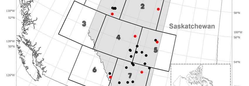
Remote Sens. 2021, 13, 900                                                                                         3 of 19

                             A shortfall of these statistical downscaling methods is that few of them presented spatially
                             downscaled GRACE data in a gridded format which resembles aquifers more closely and
                             is perhaps the most useful for investigating spatial patterns in groundwater storage and
                             abstraction [42].
                                   In an attempt to downscale GRACE TWSA in a gridded format which closely re-
                             sembles a high resolution TWS product simulated by a LSM, Zhong et al. [34] presented
                             an iterative adjustment method based on the self-calibration variance-component model
                             (SCVCM) for generating high spatial resolution total water storage anomaly (TWSA)
                             through combination of GRACE observations and the TWSA simulated by the LSM Eco-
                             logical Assimilation of Land and Climate Observations (EALCO). Using the SCVCM, the
                             GRACE-derived total water storage anomaly (GRACE TWSA) can be spatially downscaled
                             from its original coarse resolution (3-degree spherical cap/~300 km) to a high spatial
                             resolution (5 km) grid [34].
                                   After the GRACE TWSA is downscaled to a high spatial resolution grid spatially,
                             another challenge is how to further downscale it from monthly to daily frequency tempo-
                             rally. For the very first time, we extended the iterative adjustment method based on the
                             self-calibration variance-component model (SCVCM) to downscale spatiotemporally the
                             monthly coarse resolution GRACE TWSA to daily 5 km resolution of the EALCO TWSA in
                             this study. This new method combines the spatially downscaled GRACE TWSA with daily
                             EALCO TWSA to generate a high spatiotemporal resolution TWSA product. In following,
                             we first introduce the newly developed SCVCMs for the spatiotemporal downscaling
                             of GRACE TWSA in Section 2. Then, a test case including data processing and model
                             evaluation methods is presented in Section 3. After that, the results are evaluated and
                             discussed in Section 4. Finally, we conclude this study with a summary in Section 5.

                             2. Methodology
                             2.1. Problem Description
                                   The objective of this study is to downscale GRACE TWSA from its original coarse
                             resolution (monthly, ~300 km) grid to the high spatiotemporal resolution (daily, 5 km)
                             grid of the LSM EALCO TWSA through a data combination and adjustment model. Let G
                             denote the GRACE TWSA observation of a mascon, i.e., the mascon average of a period
                             of M days (about one month) and t be the time in days from 1 to M. For a grid point i
                             (e.g., a 5 km × 5 km grid cell used for the LSM EALCO simulation within the mascon), let
                             Li (t) be the EALCO TWSA at time t. Then, all observations available for a mascon and an
                             observation period of about a month are

                                                    tij , Lij = Li tij , G, 1 ≤ j ≤ M, 1 ≤ i ≤ N                   (1)

                             where tij denotes the day j for the grid point i, M is the number of the daily EALCO TWSA
                             for the grid point i (i.e., the total number of days used for deriving the GRACE TWSA G,
                             usually about a month), and N is the total grid cells within the mascon.
                                  Now, the objective is to build a model or to develop a process that can downscale the G
                             from its original coarse resolution of mascon grid to a high spatiotemporal resolution grid
                             of the EALCO TWSA Li (t) through data combination and adjustment of the observations
                             G and Li (t).
                                  For a very first attempt, we suggest a two-step method. In the first step, an iterative
                             adjustment method based on the self-calibration variance-component model (SCVCM) is
                             used to downscale the monthly GRACE TWSA G spatially to the high spatial resolution
                             grid of the EALCO TWSA Li (t). In the second step, the spatially downscaled GRACE TWSA
                             (SD TWSA) Gi at each grid point i is further downscaled temporally to daily by using a
                             second SCVCM for combination of the SD TWSA Gi and the daily EALCO TWSA Lij .

                             2.2. The SCVCM for Spatial Downscaling of the GRACE TWSA
                                  For the spatial downscaling of the GRACE TWSA from its coarse resolution mascon
                             grid to the high-resolution grid of the EALCO TWSA, Zhong et al. [34] presented an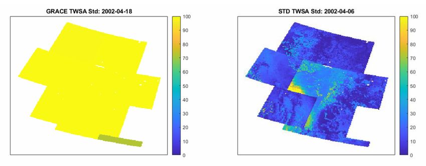
Remote Sens. 2021, 13, 900                                                                                             4 of 19

                             iterative combination adjustment method based on the SCVCM [45]. The method takes the
                             monthly GRACE TWSA G of a mascon and the monthly averaged EALCO TWSA at each
                             grid point i, which includes soil water content, snow water equivalent, and plant water
                             as input observations with unknown uncertainties, and then establishes an observation
                             system to estimate the unknown TWSA at the high-resolution grid points. To consider
                             the missing groundwater storage (GWS) and surface water storage (SWS), which are not
                             included in the EALCO TWSA, or simply the systematic differences between the GRACE
                             TWSA and the EALCO TWSA, an additional systematic parameter for each grid point is
                             introduced to the system and estimated through an iterative adjustment process with a
                             posteriori variance-component estimation technique. Following the process described in
                             Zhong et al. [34], the final model outputs are spatially downscaled TWSA (SD TWSA) at
                             the high spatial resolution grid. We take the same model and process directly as the first
                             step of our downscaling processing in this study.

                             2.3. The SCVCM for Temporal Downscaling of the GRACE TWSA
                                  After the GRACE TWSA is spatially downscaled to the high spatial resolution (5 km)
                             grid in the first step, the next objective of this study is to downscale the SD TWSA Gi at
                             each grid point i further from its temporal resolution monthly to the daily resolution of
                             the EALCO TWSA Lij . This can be realized by applying a similar method for the spatial
                             downscaling of the GRACE TWSA in the first step.
                                  Similar to the SCVCM development for the spatial downscaling, we have to take
                             the following three particular challenges into account to build up a new SCVCM for
                             temporal downscaling of the SD TWSA. First, the model must be able to distribute the
                             information from a single monthly coarse-temporal observation onto the M daily finer-
                             temporal model elements properly. Second, the damped signal or leakage errors of the
                             SD TWSA introduced through the monthly average smoother must be handled properly
                             prior to or during the combination adjustment process. Third, the systematic differences
                             between the EALCO TWSA and SD TWSA must be considered or compensated. Otherwise,
                             the data combination may introduce errors to or reduce the accuracy of the model outputs.
                                  Assume that the SD TWSA Gi at a grid point i equals to the average of the M daily
                             observations Gij which are to be determined, then our objective is to restore Gij from the
                             monthly averaged signal Gi . Similar to the gridded scale gain factor k i introduced to restore
                             the leakage errors [46] or the damped signal from the mascon averaged GRACE TWSA G
                             in the SCVCM modeling for the spatial downscaling [34], we define a scale gain factor k ij
                             for each day to restore the leakage errors or the damped signal from the monthly averaged
                             SD TWSA Gi . Then we can restore Gij from Gi as follows

                                                 Gij = k ij Gi + ε ij , i = 1, 2, . . . , N        j = 1, 2, . . . M      (2)

                             where ε ij are the misfit between the daily (i.e., unaveraged) Gij and the smoothed (i.e., aver-
                             aged) monthly signal Gi . From Equation (2), the gain factor k ij plays a role of distributing
                             the single monthly coarse-temporal observation Gi onto the M daily finer-temporal model
                             elements Gij .
                                  If we think that the monthly average smoother used for averaging both the daily SD
                             TWSA and the daily LSM EALCO TWSA for their monthly signal values are same, we can
                             determine the scale gain factor k ij using the daily LSM EALCO TWSA Lij as follows

                                                                         Lij              M      Lij
                                                                k ij =
                                                                         Li
                                                                               ,   Li =   ∑      M
                                                                                                     .                    (3)
                                                                                          j =1

                                  Applying the scale gain factor k ij from Equation (3) to restore the damped signals or
                             leakage error of the SD TWSA Gi and introducing unknown parameter xij to denote the
                             spatiotemporally downscaled GRACE TWSA (SPTD TWSA) at time tij , then we can have
                             the following observation equation for each daily SPTD TWSA Gij = k ij Gi at time tij and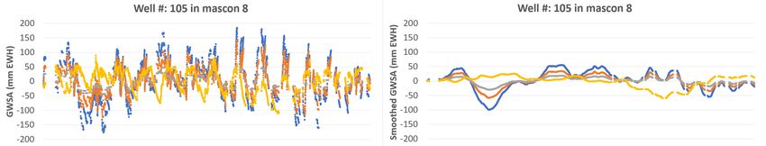
Remote Sens. 2021, 13, 900 5 of 19
the monthly averaged observation Gi = Gi (as a constraint condition they should meet
after the downscaling):
Gij = k ij Gi = xij + ε Gij , σ̂G2 = k2ij σ̂G2 ,
ij i
M (4)
Gi = ∑ xij /M + ε Gi , σ̂G2 .
j =1 i
Here, σ̂G2 is a variance estimate of the monthly averaged signal Gi , which is actually
i
the spatially downscaled SD TWSA Gi resulted from the first step, i.e., σ̂G2 = σ̂G2 .
i i
For the daily EALCO TWSA Lij , we can establish the following observation equations
by introducing an additional unknown parameter sij to model the missing groundwater
and surface water storage anomaly (GSWSA) component in Lij ,
Lij = xij − sij + ε Lij , σ̂L2ij (5)
where σ̂L2ij is a variance estimate of the daily EALCO TWSA Lij .
If we treat the xij in Equations (4) and (5) as unknown model parameters and the sij as
additional stochastic systematic parameters to be determined from the observations Gij
and Lij , Equations (4) and (5) form a typical SCVCM with two different observation types
(i.e., Gij and Lij ) and one group of stochastic systematic parameters (i.e., sij ) [45].
By defining following unknown parameter vectors,
xi1 k i1 Gi δxi1
xi2 k i2 Gi δxi2
x = xo + δx , xo = = , δx = ,
.. .. ..
. . .
xiM k iM Gi δxiM
×1
M ×1
M M ×1 (6)
0 δsi1
0 δsi2
s = so + δs, so = , δs = ,
.. ..
. .
0 M ×1
δsiM M ×1
we obtain the following model coefficient matrices and observation vectors
I M× M −I M × M
LE
A= I M× M , H = 0 M× M ,L = ,
LG (2M+1)×1 (7)
11× M /M (2M+1)× M
01 × M (2M+1)× M
T T T
LE = Li1 ··· LiM , LG = Gi1 · · · GiM Gi = k i1 Gi · · · k iM Gi Gi ,
as well as the functional model of the SCVCM
L = Aδx + Hδs + ε (8)
or equivalently as the error equations
yT = yTo + δyT , yTo = xTo sTo , δyT = δxT δsT ,
vE = BE δy − lE , lE = LE − BE yo , BE = I M× M −I M× M , ! Σ E = σE2 QEE , PE = Σ− 1
E ,
I M× M 0 M× M −1 (9)
vG = BG δy − lG , lG = LG − BG yo , BG = 11× M , Σ G = σG 2Q
GG , PG = Σ G ,
M
01× M
vs = Bs δy − ls , ls = so − Bs yo , Bs = 0 M× M I M× M , Σs = σs2 Qss , Ps = Σ− 1
s .
Following the same solution method used to the SCVCM for the spatial downscal-
ing [34], we obtain the final estimates of the parameters δx, and δs and their variance and
covariance estimates as follows: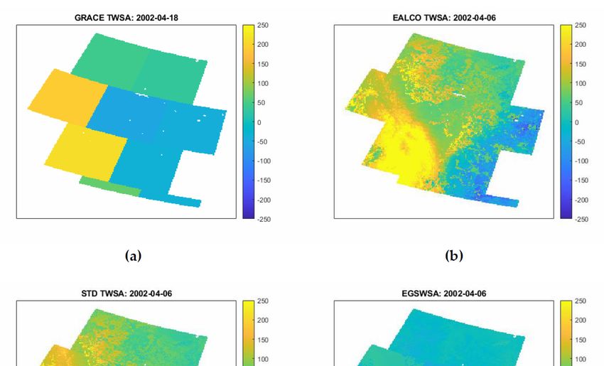
Remote Sens. 2021, 13, 900                                                                                                                               6 of 19

                                                             −1
                                  AT P L A     AT P L H                 AT P L l

                δx̂                                                                                             PE     0                            T
                          =                                                                        , PL =                      , l=     lTE   lTG         (10)
                δŝ               HT P L A    T
                                             H P L H + Ps             T
                                                                     H P L l + Ps ls                             0    PG
                                                                                                                                  −1
                                                                                                   AT P L A        AT P L H

                                                                          δx̂
                                                                Cov                 =   σ̂o2                                                              (11)
                                                                          δŝ                      HT P L A     H T P L H + Ps
                                        where σ̂o2 is an estimate of the unit weight variance

                                                                                    vTE PE vE + vG
                                                                                                 T P v + vT P v
                                                                                                    G G   s s s
                                                                          σ̂o2 =                                                                          (12)
                                                                                                   M
                                              From Equation (6), x̂ = xo + δx̂ is an estimate vector of the unknown spatiotemporally
                                        downscaled TWSA x, and the corresponding diagonal variances in the covariance matrix
                                        (11) are their accuracy or uncertainty estimates. Similarly, ŝ = so + δŝ is an estimate vector
                                        of the GSWSA parameters s and the corresponding diagonal variances in the covariance
                                        matrix (11) are their accuracy or uncertainty estimates.

                                        3. Test Case and Evaluation Methods
                                        3.1. Study Area
                                          To verify the SCVCM’s performance, we need independent TWSA observations at
                                    the high spatiotemporal resolution grid points for a comparison. However, such TWSA
                                    observations are not available. Alternatively, assuming that the surface water storage
                                    anomaly (SWSA) is ignorable in a selected dry area, then we may think that the difference
                                    between the GRACE TWSA and the EALCO TWSA, i.e., the GSWSA, is caused mainly by
                                    the groundwater storage anomaly (GWSA). Hence, if we can determine the GWSA from
                                    in-situ groundwater monitoring well (GMW) observations, then the estimated GSWSA
                                    parameter, ŝi , should be comparable with the observed GWSA at the same location. There-
                                    fore, for the model evaluation, we selected a study region located in the dry region of
                                    Canada’s Prairie where surface water is a less significant factor in the TWS than
Remote Sens. 2021, 13, x FOR PEER REVIEW                                                                            7 of other
                                                                                                                         20
                                    components. The test area covers 7 full and 2 partial mascons in the province of Alberta,
                                    Canada (Figure 1).

                                                    Map
                                        Figure1.1.Map
                                       Figure         for for
                                                          the the   test region.
                                                               test region. There There  are 32 unconfined
                                                                                  are 32 unconfined or semi- or semi-unconfined
                                                                                                             unconfined            groundwater
                                                                                                                         groundwater    moni-
                                       toring wells (dots) in the 9 mascons (numbered from 1 to 9) over the study region locatedlocated
                                        monitoring  wells  (dots)  in the 9 mascons  (numbered  from 1 to 9) over the study region  in the in the
                                        provinceofofAlberta,
                                       province      Alberta,Canada.
                                                               Canada.

                                       3.2. Data and Data Processing
                                       3.2.1. GRACE TWSA Data
                                             Same as the GRACE TWSA data used for Zhong et al. [34], we take the monthly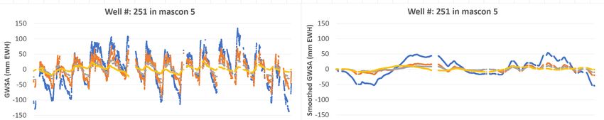
Remote Sens. 2021, 13, 900                                                                                          7 of 19

                             3.2. Data and Data Processing
                             3.2.1. GRACE TWSA Data
                                  Same as the GRACE TWSA data used for Zhong et al. [34], we take the monthly
                             GRACE TWS product (RL06 V1.0) from the JPL mascon solution [47–49] as one of our
                             input observations for this study. In order to make it comparable with the EALCO TWSA
                             data, a new baseline value, the mean from 5 April 2002 to 31 December 2016, is deducted
                             from the raw data downloaded from the JPL TWS product website (https://grace.jpl.nasa.
                             gov/data/get-data/jpl_global_mascons/, last access: on 28 July 2020). That means that
                             the input GRACE TWSA observations for this study are the monthly TWSA derived from
                             the JPL mascon solution by deducting the new baseline value. Its temporal resolution is
                             monthly, and its spatial resolution is the JPL mascon grid (~300 km).

                             3.2.2. EALCO TWSA Data
                                  The EALCO TWSA data used for this study are also similar to the data used in
                             Zhong et al. [34]. Details about the LSM EALCO refer to [50–62]. For this study, we first
                             calculated the daily EALCO TWS from the 30-minute simulations for soil water, snow
                             water equivalent, and plant water for each EALCO grid cell at 5 km × 5 km for the period
                             corresponding to GRACE observations from 5 April 2002 to 31 December 2016. The daily
                             EALCO TWSA is obtained by deducting its mean (baseline) values from 5 April 2002 to
                             31 December 2016. The EALCO simulation doesn’t include the groundwater and surface
                             water. Hence, the input EALCO TWSA observations used in this study only include soil
                             water, snow water equivalent, and plant water.

                             3.2.3. GWSA from GMW Observations
                                  Similar to the GWSA data used in Zhong et al. [34], we selected 32 unconfined or
                             semi-confined GMWs (see the black and red dots in Figure 1) in the study area and obtained
                             their daily groundwater water level observations from the GMW network of the Alberta
                             Environment and Parks, Government of Alberta (http://environment.alberta.ca/apps/
                             GOWN/#, last access: 14 November 2020). The 32 GMWs are selected due to their longest
                             monitoring period and their greatest overlap with the GRACE data. The minimum number
                             of days with available observations is 3620 of 5385 days in total (67.2%). Among them, 28
                             of the 32 GMWs (87.5%) have more than 3993 of 5385 days (74.2%) with observations. More
                             information about these GMWs is available from the website of the Alberta Environment
                             and Parks, Government of Alberta.
                                  By matching the GMW observations for the same periods used for deriving the
                             GRACE TWSA and then deducting its baseline value, we obtained the daily GMW level
                             height variations. As the GMW level height observations are not directly comparable with
                             the GRACE TWSA [63], they are multiplied by a specific yield of 5% for all 32 GMWs to
                             convert them to GWSA. The adopted specific yield 5% is a close to the mean value derived
                             by performing a least-squares fit between the daily GMW level height variations δh(tij )
                             and the corresponding estimated parameter value s(tij ) for the individual GMW i. That is,

                                                       s(tij ) = yi δh(tij ) + ε sij , i = 1, 2, . . . Mi            (13)

                             where ε sij are the misfit between s(tij ) and δh(tij ). Mi is the number of the GMW observa-
                             tions available at time tij in the grid cell i.

                             3.3. Evaluation Methods
                                  As discussed in Zhong et al. [34], the determination of the GWSA from in-situ GMW
                             level observations is a technical challenge of the model evaluation because it depends on
                             accurate specific yield information required to convert the groundwater level changes to
                             GWSA [63]. The aquifer settings and human activities such as withdrawal, injection, min-
                             ing, etc. around a GMW can largely affect the accuracy of the local GWSA determination,
                             too. In addition, the simulation errors of the input EALCO TWSA and seasonal surface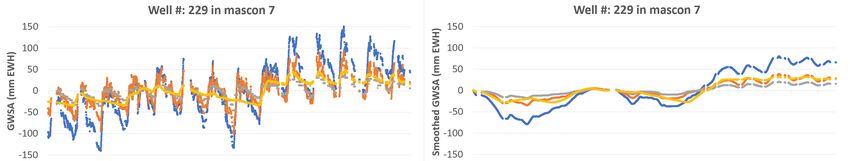
Remote Sens. 2021, 13, 900                                                                                                 8 of 19

                             water influences, etc. may cause significant differences of the estimated GSWSA for a
                             representation of the actual GWSA. Therefore, it is difficult and not practical to compare
                             the estimated GSWSA against the observed GWSA from GMW observations qualitatively
                             for the model evaluation. A more practical way is to quantitatively compare the trend
                             changes between the time series of the estimated GSWSA and the observed GWSA at the
                             GMW’s location [34]. For convenience, we name the estimated GSWSA as EGSWSA and
                             the GSWA derived from in-situ GMW level observations as observed GWSA (OGWSA) in
                             following model evaluation respectively.
                                  For evaluation of the trend changes agreement between two time series X = x1 , x2 , . . . , xn ,
                             Y = y1 , y2 , . . . , yn , simple and effective comparison indicators are the root mean square
                             difference (RMSD) and Person’s correlation coefficient (PCC) [64]:
                                                                            s
                                                                                 n   ( x − y )2
                                                                 RMSD =        ∑ i =1 i n i                                 (14)

                                  Pearson’s correlation

                                                                         ∑in=1 ( xi − x )(yi − y)
                                                        PCC = q                        q                                     (15)
                                                                      n
                                                                    ∑ i =1 ( i
                                                                            x  −  x ) ∑in=1 (yi − y)2
                                                                                     2

                             where xi and yi are the X and the Y time series respectively, n is the total number of
                             available observations in the time series, and x and y are the mean of xi and yi , respectively.
                                  As pointed out in Zhong et al. [34], we use the RMSD to measure the agreement
                             goodness of the EGSWSA time series against the OGWSA time series. Although its
                             definition is same as the root mean square error (RMSE) used to measure the error of a
                             model in predicting quantitative data, its meaning is different. We cannot see it as the
                             RMSE because none of the EGSWSA and the OGSWA can be treated as a true value or
                             standard for the measurement error.
                                  Following the same model evaluation methods used in Zhong et al. [34], we can also
                             compare the EGSWSA and the OGSWA not only in temporal domain but also in spatial
                             domain if we see the EGSWSAs at different GMW’s locations at a same observation time
                             as a data series. In temporal domain, we compare the EGSWSA and the OGSWA time
                             series for a GMW along the entire observation period. In spatial domain, we compare the
                             EGSWSA and the OGSWA for different GMWs at a specific observation time. In addition,
                             we can evaluate the model output through the estimated uncertainty by the model self too.
                             If the estimated uncertainty of the SPTD TWSA from Equation (11) is comparable with
                             the a priori input uncertainty of the GRACE TWSA and the EALCO TWSA, this means
                             the model outputs are reasonable. From the estimated uncertainty information, we can
                             also infer the quality of input observations and how well they fit with each other at an
                             observation time within a mascon. For the time series of the SPTD TWSA, we can also
                             compare their uncertainties at different observation times.
                                  Since the main factors that influence the quality of the EALCO TWSA include the dis-
                             parity in forcing data, modelling methods, and parameters used for the EALCO simulation,
                             and the uncertainty of the resultant EALCO TWSA is the major error source that impacts
                             the uncertainty of the SPTD TWSA, a posteriori uncertainty analysis of the SPTD TWSA
                             can also help us better inform accuracy of the EALCO TWSA and identify where and when
                             the input data needs to be improved for a better model output.

                             4. Results and Discussions
                             4.1. Downscaled TWSA
                                    For a visual inspection on the downscaled GRACE TWSA, we plotted the input data,
                             i.e., the monthly GRACE TWSA and the daily EALCO TWSA, against the output data,
                             i.e., the spatiotemporally downscaled daily TWSA (SPTD TWSA) and the estimated daily
                             EGSWSA in Figure 2.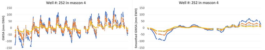
4.1. Downscaled TWSA
                                    For a visual inspection on the downscaled GRACE TWSA, we plotted th
                             i.e., the monthly GRACE TWSA and the daily EALCO TWSA, against the ou
Remote Sens. 2021, 13, 900   the spatiotemporally downscaled daily TWSA (SPTD TWSA) and9the of 19 estima

                             SWSA in Figure 2.

                              Figure 2. Animated illustration of the input data: (a) the monthly GRACE TWSA and (b) the daily
                             Figure   2. Animated illustration of the input data: (a) the monthly GRACE TWSA an
                              EALCO TWSA, against the output data: (c) the spatiotemporally downscaled daily TWSA (SPTD
                             EALCO       TWSA, against the output data: (c) the spatiotemporally downscaled daily T
                              TWSA) and (d) the estimated daily GSWSA from April 5, 2002 to December 31, 2016. GRACE
                             TWSA)      and (d)
                              TWSA, Gravity      the estimated
                                              Recovery  and Climatedaily    GSWSA from
                                                                      Experiment-derived      April
                                                                                           Total Water5,Storage
                                                                                                         2002 to  December
                                                                                                                Anomaly; TWSA,31, 2016
                             TWSA,     Gravity
                              Total Water Storage Recovery     and Climate
                                                  Anomaly; EALCO                Experiment-derived
                                                                      TWSA, Ecological                      Total
                                                                                         Assimilation of Land     Water Obser-
                                                                                                              and Climate Storage Ano
                             vations Terrestrial Water Storage Anomaly; EGSWSA, Estimated Groundwater and Surface Water
                             Storage Anomaly.

                                  From Figure 2, we can see that the suggested method is capable to downscale the
                             GRACE TWSA from its original coarse-resolution (monthly ~300 km) to the high spa-
                             tiotemporal resolution (daily 5 km) grid of the EALCO TWSA. The spatial patterns of the
                             SPTD TWSA are similar to the EALCO TWSA. This indicates that the SPTD TWSA is just
                             an adjusted EALCO TWSA by the EGSWSA. For a quick validation, it is clear that the
                             SPTD TWSA had been changing from 2002 to 2016 and this change is especially significant
                             in the southwest region marked as mascon 3, 6, and 8. The reasons for these changes
                             are multiplex. Some changes can be explained as the effects of extreme droughts and
                             floods occurred in this region, for instances, 2013 Alberta Floods [65–67] caused the TWSA
                             increases in Southern Alberta in June 2013. In comparison to the TWSA’s changes, the
                             EGSWSA are relatively small and stable (Figure 2d). Some visible changes happened in
                             the region marked as mascon 4, 7, and 8 from 2013 to 2016. Those relatively small changes
                             of the EGSWSA are consistent with the OGWSA derived from the in-situ GMW level
                             observations (more details in Section 4.3).

                             4.2. Quantitively Comparison Results
                                  To assess the model effectiveness for spatiotemporally downscaling GRACE TWSA,
                             we compared three time series of the GSWSA derived from different model outputs against
                             the 32 GMWs observations. The first time series is derived by differencing the EALCO
                             TWSA from the original GRACE TWSA without any downscaling process. We named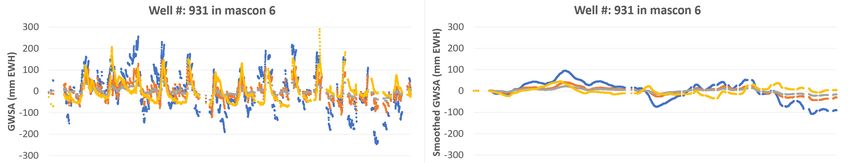
Remote Sens. 2021, 13, 900 10 of 19
this time series as EGSWSA1. The second time series is derived by differencing the
EALCO TWSA from the spatially downscaled GRACE TWSA, i.e., the SD TWSA without
conducting the temporal downscaling process. We named this time series as EGSWSA2.
The third time series are derived by conducting both the spatial and temporal downscaling
processes described in Section 3. We named it as EGSWSA3.
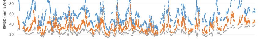
Figure 3 shows comparison plots of the RMSD (a) and the PCC (b) in temporal
domain for the 32 GMWs. It is clear that the EGSWSA3 derived from the spatiotemporal
downscaling show significantly smaller RMSD than EGSWSA1 and EGSWSA2, which are
derived from the original GRACE TWSA and the spatially downscaled GRACE TWSA, i.e.,
SD TWSA, respectively. The comparison between the EGSWSA1 and EGSWSA2 shows
that the EGSWSA2 has smaller RMSD than the EGSWSA1. However, the PCC of all three
times series did not show significant differences. They all show a very weak correlation
level. These results tell us that both the spatial and temporal downscaling processes are
helpful in reducing the RMSD between the EGSWSA and the OGWSA. They functioned
Remote Sens. 2021, 13, x FOR PEER REVIEW
like a smoothing filter in adjusting the observation errors of the EALCO TWSA and 11 ofthe
20
GRACE TWSA.
(a)
(b)
Figure 3. Comparison of the root mean square difference (RMSD) (a) and of the Pearson's Correlation Coefficients (PCC)
Figure 3. Comparison of the root mean square difference (RMSD) (a) and of the Pearson’s Correlation Coefficients (PCC) (b)
(b) in the temporal domain of the selected 32 groundwater monitoring wells in the province of Alberta, Canada. The
in the temporal domain of the selected 32 groundwater monitoring wells in the province of Alberta, Canada. The RMSD
RMSD and PCC are calculated by comparing the three GRACE derived EGSWSA time series EGSWSA1, EGSWSA2 and
and PCC areagainst
EGSWSA3 calculated by comparing
the OGWSA the three
time series GRACE
derived derived
from EGSWSA
the GMW time series
observations. TheEGSWSA1, EGSWSA2
unit of the RMSD (a)and EGSWSA3
is mm EWH.
against the OGWSA time series derived from the GMW observations. The unit of the RMSD (a)
GRACE, Gravity Recovery and Climate Experiment; EGSWSA, Estimated Groundwater Storage Anomaly; OGWSA, is mm EWH. GRACE,
Ob-
GravityGroundwater
served Recovery and Climate
Storage Experiment;
Anomaly; EWH,EGSWSA, Estimated
Equivalent Groundwater Storage Anomaly; OGWSA, Observed
Water Height.
Groundwater Storage Anomaly; EWH, Equivalent Water Height.
Figure 4 shows comparison plots of the RMSD (a) and the PCC (b) along the GRACE
observation time domain from April 5 to December 31, 2016. It is clear that the EGSWSA3
derived from the spatiotemporal downscaling give smaller RMSD for almost all the time
epochs than the EGSWSA1 and EGSWSA2. This result demonstrated that the SPTD TWSARemote Sens. 2021, 13, 900 11 of 19
Figure 4 shows comparison plots of the RMSD (a) and the PCC (b) along the GRACE
observation time domain from 5 April to 31 December 2016. It is clear that the EGSWSA3
derived from the spatiotemporal downscaling give smaller RMSD for almost all the time
epochs than the EGSWSA1 and EGSWSA2. This result demonstrated that the SPTD TWSA
is better than the SD TWSA while the SD TWSA is better than the original GRACE TWSA.
Remote Sens. 2021, 13, x FOR PEER REVIEW 12 of 20
From this point view, the suggested downscaling processes made a sense.
(a)
(b)
Figure 4. Comparison
Figure 4. Comparisonof the Root
of the Mean
Root MeanSquare
SquareDifference (RMSD)(a)
Difference (RMSD) (a)and
andthethe Pearson's
Pearson’s Correlation
Correlation Coefficients
Coefficients (PCC)(PCC)
(b) in(b)
theinspatial domain. The RMSD and PCC are calculated by comparing the three GRACE derived GWSA
the spatial domain. The RMSD and PCC are calculated by comparing the three GRACE derived GWSA time series time series
EGSWSA1, EGSWSA2, and EGSWSA3 against the OGWSA time series derived from the GMW observations
EGSWSA1, EGSWSA2, and EGSWSA3 against the OGWSA time series derived from the GMW observations in the spatial in the spatial
domain, that is, from different GMWs at a same observation time. The unit of the RMSD (a) is mm EWH. GRACE,
domain, that is, from different GMWs at a same observation time. The unit of the RMSD (a) is mm EWH. GRACE, Gravity Gravity
Recovery and Climate Experiment; GWSA, Groundwater Storage Anomaly; OGWSA, Observed
Recovery and Climate Experiment; GWSA, Groundwater Storage Anomaly; OGWSA, Observed Groundwater Storage Groundwater Storage
Anomaly; GMW,
Anomaly; GMW,Groundwater
Groundwater Monitoring
MonitoringWell; EWH,Equivalent
Well; EWH, Equivalent Water
Water Height.
Height.
4.3.4.3.
Visual Comparison
Visual ComparisonResults
Results
For
Fora avisual
visualcomparison,
comparison, we we first
firstplotted
plottedscatter
scatter plots
plots of pair
of all all pair points
points forthree
for the the three
time-series
time-seriesofofEGSWSA1, EGSWSA2,
EGSWSA1, EGSWSA2, andand EGSWSA3
EGSWSA3 against
against the OGSWA
the OGSWA derived derived
from the from
the3232GMWs
GMWs in Figure 5, respectively.
in Figure FigureFigure
5, respectively. 5 shows5that the scatter
shows plot
that the of the EGSWSA3
scatter plot of the EG-
looks improved
SWSA3 and gives
looks improved anda smaller
gives aRMSD thanRMSD
smaller the EGSWSA1
than theand EGSWSA2.
EGSWSA1 andTheEGSWSA2.
PCC
looks small for all three time-series and no improvement is made
The PCC looks small for all three time-series and no improvement is made by bothby both spatial andspatial
and temporal downscaling processes. This indicates that the iterative adjustment used for
downscaling process did improve the RMSD but not the PCC. This is consistent with the
results of the quantitative evaluation above.Remote Sens. 2021, 13, 900 12 of 19
Remote Sens. 2021, 13, x FOR PEER REVIEW 13 of 20
ens. 2021, 13, x FOR PEER REVIEW temporal downscaling processes. This indicates that the iterative adjustment used for
downscaling process did improve the RMSD but not the PCC. This is consistent with the
results of the quantitative evaluation above.
Figure 5. Scatter plots of the three time-series of EGSWSA1, EGSWSA2, and EGSWSA3 derived from the GRACE TWSA
and the EALCO TWSA against the OGWSA from the 32 GMWs. GRACE TWSA, Gravity Recovery and Climate Experi-
ment-derived Total Water Storage Anomaly; EGSWSA, Estimated Groundwater and Surface Water Storage Anomaly;
OGWSA, Observed Groundwater Storage Anomaly; GMW, Groundwater Monitoring Well; EALCO, Ecological Assimi-
lation of Land and Climate Observations.
gure 5. Scatter plots of the three For visualofcomparisons
time-series EGSWSA1, ofEGSWSA2,
the trend changes of the EGSWSAs andfrom
the OGWSA time TW
Figure 5. Scatter plots of the threewe
series, time-series
plottedoftheEGSWSA1,
EGSWSA1, EGSWSA2, andand
EGSWSA2,
EGSWSA3
EGSWSA3 derived derived
and EGSWSA3 from the GRACE
against
the GRACE
TWSA
the OGWSA for the
d the EALCO and TWSA
the EALCO against the OGWSA
TWSA against the OGWSA from
fromthe 32GMWs.
GMWs. GRACE
TWSA, TWSA, GravityandRecovery and Climate Expe
selected 8 GMWs inthe 32
Figure GRACE
6. These 8 GMWs Gravity Recovery
are located in the Climate Experiment-
different mascons marked
ent-derived Total Water Storage
derived Total Water Storage Anomaly; EGSWSA, Estimated Groundwater and Surface Water Storage Anoma
Anomaly; EGSWSA, Estimated Groundwater and Surface Water Storage Anomaly; OGWSA,
as 1, 2 ,4 ,5 ,6 ,7 ,8, and 9 (see the red dots in Figure 1). There is no GWMs available in the
Observed
GWSA, Observed Groundwater Storage
Groundwater Anomaly; GMW, Groundwater Monitoring Well; EALCO, Ecological Assimilation of Land
mascon 3. Anomaly; GMW, Groundwater Monitoring Well; EALCO, Ecological Assim
Storage
and Climate Observations.
ion of Land and Climate Observations. The direct trend changes comparisons of the EGSWSAs and the OGWSA time series
in the For
left visual
Colum of Figure 6oflook
comparisons very noisy
the trend changes because of significant
of the EGSWSAs andseasonal
the OGWSAinfluences,
time
simulation,
For visual
series, or observation
comparisons
we plotted errors,
the EGSWSA1,of theetc. For a better
trend changes
EGSWSA2, trend
and EGSWSA3 comparison
of the and
EGSWSAs
against analysis,
the OGWSA we
andfortheused
theOGWS
a selected
1-year (3658 GMWsdays)inmoving
Figure 6.average
These 8 smooth
GMWs are filter to deseasonalize
located some
in the different seasonal
mascons influ-
marked
series, we plotted the EGSWSA1, EGSWSA2, and EGSWSA3 against the OGWSA
as 1, and
ences 2, 4, smooth
5, 6, 7, 8,out
andsome
9 (seenoise
the red dots in
signals orFigure 1). There
observation is noThe
errors. GWMs available
smoothed in the
time series
selected 8compared
GMWs
mascon
are 3. inthe
in Figure 6. These
right Colum 8 GMWs
of Figure 6. are located in the different mascons m
as 1, 2 ,4 ,5 ,6 ,7 ,8, and 9 (see the red dots in Figure 1). There is no GWMs availabl
mascon 3.
The direct trend changes comparisons of the EGSWSAs and the OGWSA tim
in the left Colum of Figure 6 look very noisy because of significant seasonal infl
simulation, or observation errors, etc. For a better trend comparison and analysis, w
a 1-year (365 days) moving average smooth filter to deseasonalize some seasona
ences and smooth out some noise signals or observation errors. The smoothed tim
are compared in the right Colum of Figure 6.
Figure 6. Cont.Remote Sens. 2021, 13, 900 13 of 19
Remote Sens. 2021, 13, x FOR PEER REVIEW 14 of 20
Figure 6. Cont.Remote Sens. 2021, 13, 900 14 of 19
Remote Sens. 2021, 13, x FOR PEER REVIEW 15 of 20
Figure 6. Trend
Figure 6. Trendcomparisons
comparisons ofofthe
theGRACE
GRACEderived
derivedGWSA
GWSA timetime series EGSWSA1,EGSWSA2,
series EGSWSA1, EGSWSA2,and andEGSWSA3
EGSWSA3 against
against thethe
OGWSA derived from 8 selected GMWs which are located in 8 different mascons. The left column compares
OGWSA derived from 8 selected GMWs which are located in 8 different mascons. The left column compares the unfilteredthe unfiltered
data andand
data thethe
right column
right columnshows
shows the
thesmoothed
smootheddata
databybyaa1-year
1-year (365
(365 days) movingaverage
days) moving averagefilter.
filter.GRACE
GRACE TWSA,
TWSA, Gravity
Gravity
Recovery and Climate Experiment-derived Total Water Storage Anomaly; EGSWSA, Estimated Groundwater and Surface
Recovery and Climate Experiment-derived Total Water Storage Anomaly; EGSWSA, Estimated Groundwater and Surface
Water Storage Anomaly; GWSA, Groundwater Storage Anomaly; OGWSA, Observed Groundwater Storage Anomaly;
Water Storage Anomaly; GWSA, Groundwater Storage Anomaly; OGWSA, Observed Groundwater Storage Anomaly;
GMW, Groundwater Monitoring Well; EALCO, Ecological Assimilation of Land and Climate Observations.
GMW, Groundwater Monitoring Well; EALCO, Ecological Assimilation of Land and Climate Observations.
From Figuretrend
The direct 6, wechanges
can seecomparisons
that the variationof the ranges
EGSWSAs of three unfiltered
and the OGWSAEGSWSAs
time seriesare
much
in thebigger than the
left Colum OGWSA.
of Figure 6 lookTheir
veryamplitude of individual
noisy because observation
of significant seasonallooks not com-
influences,
parable. The reasons
simulation, for theerrors,
or observation big differences may be
etc. For a better multifaceted.
trend comparisonAs andmentioned
analysis, wein Section
used
4.3, it might
a 1-year (365bedays)
caused by inaccurate
moving average smoothspecific yield
filter used to convert
to deseasonalize some the GMW influences
seasonal level height
and smooth
changes to OGWSAout someor noise signals
possible or observation
simulation errors in errors. The smoothed
the input EALCO TWSA time series are
or signifi-
compared
cant seasonal in SWSA
the rightcaused
Columby of something
Figure 6. such as floods, etc. This is why it is still not
From
practical Figure 6,the
to compare weamplitudes
can see thatofthe thevariation
EGSWSAranges and the of OGWSA
three unfiltered EGSWSAs
qualitatively for the
model evaluation. However, if we compare their long-term trend changes, thelooks
are much bigger than the OGWSA. Their amplitude of individual observation not
EGSWSA3
comparable. The reasons for the big differences may be multifaceted.
shows a better trend change agreement than the EGSWSA1 and EGSWSA2 for all selected As mentioned in
Section 4.3, it might be caused by inaccurate specific yield used to convert the GMW level
GMWs except for very few GMWs, especially after deseasonalizing by the 1-year (365
height changes to OGWSA or possible simulation errors in the input EALCO TWSA or
days) moving average filter. This conclusion is valid for most of the 32 GMWs. Only a few
significant seasonal SWSA caused by something such as floods, etc. This is why it is still not
of the GMWs showed some reversed results. An exception among the 8 GMWs is the well
practical to compare the amplitudes of the EGSWSA and the OGWSA qualitatively for the
W229
model inevaluation.
mascon 7, However,
which shows if we that
comparethe EGSWSA2
their long-termis closer
trendto the OGWSA.
changes, The well
the EGSWSA3
W287 and W117, which show negative correlations in Figure
shows a better trend change agreement than the EGSWSA1 and EGSWSA2 for all selected 3, have similar results. The
reason
GMWsfor this for
except result
veryisfew
notGMWs,
clear yet. Possibly,
especially afterthese exceptional
deseasonalizing bywells have(365
the 1-year a different
days)
specific
moving yield fromfilter.
average othersThisorconclusion
its OGWSA may not
is valid adequately
for most of the 32represent
GMWs. Only eithera few
the ground-
of the
water
GMWs response
showedorsomethe EGSWSA becauseAn
reversed results. of exception
unknownamong aquiferthe settings
8 GMWs andishuman
the wellactivities
W229
such as withdrawal,
in mascon 7, whichinjection,
shows that mining, etc.
the EGSWSA2 is closer to the OGWSA. The well W287
and W117, which show negative correlations in Figure 3, have similar results. The reason
forUncertainty
4.4. this result is not clear yet.
Comparison Possibly, these exceptional wells have a different specific
Results
yield
Tofrom others
evaluate theormodel
its OGWSA may not
uncertainty, weadequately
comparedrepresent either
the a priori the uncertainties
input groundwater of
response or the EGSWSA because of unknown aquifer settings and human activities such
the monthly GRACE TWSA against the uncertainties of the downscaled daily SPTD
as withdrawal, injection, mining, etc.
TWSA in Figure 7.
4.4. Uncertainty Comparison Results
To evaluate the model uncertainty, we compared the a priori input uncertainties of the
monthly GRACE TWSA against the uncertainties of the downscaled daily SPTD TWSA in
Figure 7.
Figure 7 shows that the uncertainties of the SPTD TWSA estimated by the SCVCM are
usually improved for the most times and the most parts in the test region in comparison to
the a priori input uncertainties of the original GRACE TWSA. This result indicates that the
GRACE TWSA and the EALCO TWSA fit each other well for the most times and the most
parts in the test region and the proposed method is beneficial to reduce the uncertainties.
From Figure 7, we can also see that the uncertainties of the SPTD TWSA are enlarged
sometimes at some parts to a significant extent. For instance, in May and June of 2006,
the estimated uncertainties for the region of mascon 6 are significantly larger than the a
Figure 7. Comparison of the a priori uncertainties of the input GRACE TWSA against the uncertainties of the downscaled
daily SPTD TWSA estimated by the SCVCM from April 2002 to December 2016. The unit of the uncertainties is mm EWH.of the GMWs showed some reversed results. An exception among the 8 GMWs is the w
W229 in mascon 7, which shows that the EGSWSA2 is closer to the OGWSA. The w
W287 and W117, which show negative correlations in Figure 3, have similar results. T
reason for this result is not clear yet. Possibly, these exceptional wells have a differe
Remote Sens. 2021, 13, 900 15 of 19
specific yield from others or its OGWSA may not adequately represent either the groun
water response or the EGSWSA because of unknown aquifer settings and human activit
such as withdrawal, injection, mining, etc.
priori input uncertainties of the GRACE TWSA. This indicates very possibly that there are
significant differences between the GRACE TWSA and the EACLCO TWSA input data
4.4. Uncertainty Comparison
during that period Results
in the area in question. Further analysis and quality control are needed
To evaluate the model uncertainty,
to improve the quality of the we compared
model outputs. thechanges
Similar pattern a prioriorinput uncertainties
improvement
variations of the estimated uncertainties appear not only spatially
the monthly GRACE TWSA against the uncertainties of the downscaled daily SPT but also temporally.
These results demonstrated well the role of the SCVCM as a quality control and analysis
TWSA in Figure 7.
tool for the LSM EALCO TWS simulation and GRACE observations.
Figure 7. Comparison of the a priori uncertainties of the input GRACE TWSA against the uncertainties of the downscaled
Figure 7. Comparison of the a priori uncertainties of the input GRACE TWSA against the uncertainties of the downscaled
daily SPTD TWSA estimated by the SCVCM from April 2002 to December 2016. The unit of the uncertainties is mm
daily SPTDEWH.
TWSA estimated by the SCVCM from April 2002 to December 2016. The unit of the uncertainties is mm EWH.
GRACE TWSA, Gravity Recovery and Climate Experiment-derived Total Water Storage Anomaly; SPTD TWSA,
Spatiotemporally Downscaled Total Water Storage Anomaly; GSWSA, Groundwater and Surface Water Storage Anomaly.
SCVCM, Selfcalibration Variance-Component Model; EWH, Equivalent Water Height.
From our test computations with different a priori variances (σE2 , σG2 and σ 2 ) assigned to
S
the observation Lij , Gij , and the apriori value so (zero as virtual observation of the parameter
si ) in Equation (9), we found that the uncertainties of the model outputs vary to some extent.
These a priori variance settings will impact the convergence speed of the iterative adjustment
too. For a fast convergence, equal weighting with QEE = σ̂E2 I, QGG = σ̂G2 I and QSS = σ̂S2 I is
recommended. For improvement of the model outputs, more advanced weighting options
based on the improved accuracy estimation of the GRACE TWSA (e.g., [46]) and the EALCO
TWSA may be explored in future studies.
5. Conclusions
In this study, we presented a two-step method for downscaling GRACE-derived total
water storage anomaly (GRACE TWSA) from its original coarse resolution (monthly, 3-
degree spherical cap/~300 km) to a higher spatio-temporal resolution (daily, 5 km) using
the land surface model (LSM) simulated high spatiotemporal resolution terrestrial water
storage anomaly (LSM TWSA). In the first step, an iterative adjustment method based on
the self-calibration variance-component model (SCVCM) is used to downscale the monthly
GRACE TWSA spatially to the higher resolution grid used for the LSM simulation. In
the second step, the spatially downscaled monthly GRACE TWSA is further downscaled
using the daily LSM TWSA to generate finer temporal resolution TWSA. By applying
the method to produce high spatiotemporal resolution TWSA through combination of
the monthly coarse resolution (~300 km) GRACE TWSA from the JPL (Jet Propulsion
Laboratory) mascon solution and the daily high resolution (5 km) LSM TWSA from the
Ecological Assimilation of Land and Climate Observations (EALCO) model, we evaluated
its benefit and effectiveness by comparing the estimated groundwater and surface water
storage anomaly (EGSWSA) against the observed groundwater storage anomaly (OGWSA)Remote Sens. 2021, 13, 900 16 of 19
by assuming that the surface water in a dry test region is ignorable. From the evaluation
results, we can draw following conclusions.
First, the proposed method is capable to downscale GRACE-derived total water
storage anomaly (GRACE TWSA) from its original monthly coarse resolution (monthly,
~300 km) to the higher spatiotemporal resolution (daily, 5 km) by combining or integrating
the high resolution EALCO TWSA. The evaluation results show that the EGSWSA by the
proposed method agrees better with the OGWSA in both temporal and spatial domain than
the GSWSA derived from the original GRACE TWSA and the spatially downscaled GRACE
TWSA. These results indicate that the proposed method makes sense and is beneficial.
Second, in comparison to most of the developed GRACE TWSA combination or
assimilation methods, the proposed method will deliver not only high spatiotemporal
resolution TWSA and GSWSA estimate at each grid point but also their internal accuracy,
i.e., estimated variance or uncertainty. From the uncertainty information, we can inform
potential quality issues in the LSM EALCO TWSA and/or the GRACE TWSA, and how
well they fit with each other in both temporal and spatial domain within a mascon. This
means the proposed method can be used as a quality control and analysis tool for the LSM
EALCO TWS simulation and the GRACE observations.
From this study, we recognized that it is still a challenge to evaluate the model’s
performance qualitatively because of the lack of accurate and comparable TWSA observa-
tions. We used the groundwater monitoring well (GMW) level observations to evaluate
the model’s performance quantitatively through comparison of the trend changes of the
estimated GSWSA and the observed GWSA. However, this evaluation is only quantitative
and not qualitative. It is also based on the assumption that the surface water in a dry
test region is ignorable. To improve the quality of the final TWSA product, the key is
to improve the quality of the input observations, i.e., either enhancing the quality of the
LSM EALCO TWS simulation or introducing more observations such as the observed
GWSA and SWSA, the simulated TWSA by different LSMs, etc. directly into the SCVCM
to constraint the LSM simulation errors. The proposed SCVCM offers such a model for
combining different observations.
Author Contributions: Conceptualization, S.W. and D.Z.; methodology, D.Z.; software, D.Z.; valida-
tion, D.Z., S.W. and J.L.; formal analysis, D.Z.; investigation, D.Z.; resources, S.W.; data curation, D.Z.,
S.W. and J.L.; writing—original preparation, D.Z.; review and editing, S.W. and J.L.; visualization,
D.Z. and J.L.; supervision, S.W.; project administration, S.W.; funding acquisition, S.W. All authors
have read and agreed to the published version of the manuscript.
Funding: This study is a part of the research and development project “The Cumulative Effects
Project and Climate Change Geoscience Program” funded by Natural Resources Canada.
Data Availability Statement: The data used in this study are openly available and can be down-
loaded from the following links: the GRACE TWS product (RL06 V1.0) https://grace.jpl.nasa.gov/
data/get-data/jpl_global_mascons/, last access: on 28 July 2020; the GMW level height observations
http://environment.alberta.ca/apps/GOWN/#, last access: 14 November 2020 and the EALCO TWS
data http://dx.doi.org/10.17632/fjt98ptgmb.1, last access: 25 February 2021. A Matlab prototype
program used for the computation is available from https://github.com/dzhong-hub/SCVCM, last
access: 25 February 2021.
Acknowledgments: Authors would like to thank anonymous reviewers for their insightful review
of and valuable comments on the manuscript, which helped to improve the quality of the paper.
Conflicts of Interest: The authors declare no conflict of interest.
References
1. Rodell, M.; Chen, J.; Kato, H.; Famiglietti, J.S.; Nigro, J.; Wilson, C.R. Estimating groundwater storage changes in the Mississippi
River basin (USA) using GRACE. Hydrogeol. J. 2006, 15, 159–166. [CrossRef]
2. Moradkhani, H.; Hsu, K.-L.; Gupta, H.V.; Sorooshian, S. Uncertainty assessment of hydrologic model states and parameters:
Sequential data assimilation using the particle filter. Water Resour. Res. 2005, 41, 05012. [CrossRef]Remote Sens. 2021, 13, 900 17 of 19
3. Wood, E.F.; Roundy, J.K.; Troy, T.J.; Van Beek, L.P.H.; Bierkens, M.F.P.; Blyth, E.; De Roo, A.; Döll, P.; Ek, M.; Famiglietti, J.; et al.
Hyperresolution global land surface modeling: Meeting a grand challenge for monitoring Earth’s terrestrial water. Water Resour.
Res. 2011, 47, 05301. [CrossRef]
4. Li, B.; Rodell, M.; Zaitchik, B.F.; Reichle, R.H.; Koster, R.D.; Van Dam, T.M. Assimilation of GRACE terrestrial water storage into a
land surface model: Evaluation and potential value for drought monitoring in western and central Europe. J. Hydrol. 2012, 2012,
103–115. [CrossRef]
5. Wang, S.; Yang, Y.; Luo, Y.; Rivera, A.A. Spatial and seasonal variations in evapotranspiration over Canada’s landmass. Hydrol.
Earth Syst. Sci. 2013, 17, 3561–3575. [CrossRef]
6. Koster, R.D.; Suarez, M.J.; Ducharne, A.; Stieglitz, M.; Kumar, P. A catchment based approach to modeling land surface pro-cesses
in a general circulation model. 1. Model structure. J. Geophys. Res. 2000, 105, 24809–24822. [CrossRef]
7. Niu, G.-Y.; Yang, Z.-L.; Dickinson, R.E.; Gulden, L.E.; Su, H. Development of a simple groundwater model for use in climate
models and evaluation with Gravity Recovery and Climate Experiment data. J. Geophys. Res. Space Phys. 2007, 112, 07103.
[CrossRef]
8. Miguez-Macho, G.; Fan, Y.; Weaver, C.P.; Walko, R.; Robock, A. Incorporating water table dynamics in climate modeling: 2.
Formulation, validation, and soil moisture simulation. J. Geophys. Res. Space Phys. 2007, 112, 112. [CrossRef]
9. Yeh, P.J.-F.; Eltahir, E.A.B. Representation of Water Table Dynamics in a Land Surface Scheme. Part I: Model Development. J. Clim.
2005, 18, 1861–1880. [CrossRef]
10. Niu, G.-Y.; Yang, Z.-L.; Dickinson, R.E.; Gulden, L.E. A simple TOPMODEL-based runoff parameterization (SIMTOP) for use in
global climate models. J. Geophys. Res. Space Phys. 2005, 110, 21106. [CrossRef]
11. Schaake, J.C.; Koren, V.I.; Duan, Q.-Y.; Mitchell, K.; Chen, F. Simple water balance model for estimating runoff at different spatial
and temporal scales. J. Geophys. Res. Space Phys. 1996, 101, 7461–7475. [CrossRef]
12. Mitchell, K.E.; Lohmann, D.; Houser, P.R.; Wood, E.F.; Schaake, J.C.; Robock, A.; Cosgrove, B.A.; Sheffield, J.; Duan, Q.;
Luo, L.; et al. The multi-institution North American Land Data Assimilation System (NLDAS): Utilizing multiple GCIP products
and partners in a continental distributed hydrological modeling system. J. Geophys. Res. Space Phys. 2004, 109, e2003JD003823.
[CrossRef]
13. Hoerling, M.; Lettenmaier, D.; Cayan, D.; Udall, B. Reconciling projections of colorado river streamflow. South. Hydrol. 2009, 8,
20–31.
14. Jackson, C.R.; Meister, R.; Prudhomme, C. Modelling the effects of climate change and its uncertainty on UK Chalk groundwater
resources from an ensemble of global climate model projections. J. Hydrol. 2011, 399, 12–28. [CrossRef]
15. Poulin, A.; Brissette, F.; Leconte, R.; Arsenault, R.; Malo, J.-S. Uncertainty of hydrological modelling in climate change impact
studies in a Canadian, snow-dominated river basin. J. Hydrol. 2011, 409, 626–636. [CrossRef]
16. Tapley, B.D.; Bettadpur, S.; Ries, J.C.; Thompson, P.F.; Watkins, M.M. GRACE Measurements of Mass Variability in the Earth
System. Science 2004, 305, 503–505. [CrossRef]
17. Zaitchik, B.F.; Rodell, M.; Reichle, R.H. Assimilation of GRACE Terrestrial Water Storage Data into a Land Surface Model: Results
for the Mississippi River Basin. J. Hydrometeorol. 2008, 9, 535–548. [CrossRef]
18. Forman, B.A.; Reichle, R.H.; Rodell, M. Assimilation of terrestrial water storage from GRACE in a snow-dominated basin. Water
Resour. Res. 2012, 48, 01507. [CrossRef]
19. Reager, J.T.; Thomas, A.C.; Sproles, E.A.; Rodell, M.; Beaudoing, H.K.; Li, B.; Famiglietti, J.S. Assimilation of GRACE Terrestrial
Water Storage Observations into a Land Surface Model for the Assessment of Regional Flood Potential. Remote Sens. 2015, 7,
14663–14679. [CrossRef]
20. Eicker, A.; Schumacher, M.; Kusche, J.; Döll, P.; Schmied, H.M. Calibration/Data Assimilation Approach for Integrating GRACE
Data into the WaterGAP Global Hydrology Model (WGHM) Using an Ensemble Kalman Filter: First Results. Surv. Geophys. 2014,
35, 1285–1309. [CrossRef]
21. Schumacher, M.; Forootan, E.; van Dijk, A.; Schmied, H.M.; Crosbie, R.; Kusche, J.; Döll, P. Improving drought simulations within
the Murray-Darling Basin by combined calibration/assimilation of GRACE data into the WaterGAP Global Hydrology Model.
Remote Sens. Environ. 2018, 204, 212–228. [CrossRef]
22. Forman, B.A.; Reichle, R.H. The spatial scale of model errors and assimilated retrievals in a terrestrial water storage assimilation
system. Water Resour. Res. 2013, 49, 7457–7468. [CrossRef]
23. Khaki, M.; Forootan, E.; Kuhn, M.; Awange, J.; Van Dijk, A.; Schumacher, M.; Sharifi, M. Determining water storage depletion
within Iran by assimilating GRACE data into the W3RA hydrological model. Adv. Water Resour. 2018, 114, 1–18. [CrossRef]
24. Khaki, M.; Schumacher, M.; Forootan, E.; Kuhn, M.; Awange, J.; Van Dijk, A. Accounting for spatial correlation errors in the
assimilation of GRACE into hydrological models through localization. Adv. Water Resour. 2017, 108, 99–112. [CrossRef]
25. Kumar, S.V.; Zaitchik, B.F.; Peters-Lidard, C.D.; Rodell, M.; Reichle, R.; Li, B.; Jasinski, M.; Mocko, D.; Getirana, A.;
de Lannoy, G.; et al. Assimilation of Gridded GRACE Terrestrial Water Storage Estimates in the North American Land Data
Assimilation System. J. Hydrometeorol. 2016, 17, 1951–1972. [CrossRef]
26. Schumacher, M.; Kusche, J.; Döll, P. A systematic impact assessment of GRACE error correlation on data assimilation in
hydrological models. J. Geod. 2016, 90, 537–559. [CrossRef]You can also read