F3 Photovoltaic Power Forecasting Based on Weather Forecast - Czech Technical University in Prague - ČVUT DSpace
←
→
Page content transcription
If your browser does not render page correctly, please read the page content below
Bachelor Project

                   Czech
                   Technical
                   University
                   in Prague

                   Faculty of Electrical Engineering
F3                 Department of Control Engineering

Photovoltaic Power Forecasting Based on
Weather Forecast

Nikita Lupenko

Supervisor: Ing. Martin Schaefer
May 2018
ii

ZADÁNÍ BAKALÁŘSKÉ PRÁCE

I. OSOBNÍ A STUDIJNÍ ÚDAJE

     Příjmení:                    Lupenko                              Jméno: Nikita                             Osobní číslo: 452941
     Fakulta/ústav:               Fakulta elektrotechnická
     Zadávající katedra/ústav:              Katedra řídicí techniky
     Studijní program: Kybernetika a robotika
     Studijní obor:               Systémy a řízení

II. ÚDAJE K BAKALÁŘSKÉ PRÁCI
  Název bakalářské práce:
   Predikce výkonu fotovoltaické elektrárny z předpovědi počasí

  Název bakalářské práce anglicky:
   Photovoltaic Power Forecasting Based on Weather Forecast

  Pokyny pro vypracování:
   1. Research the topic of solar/PV system power forecasting with a focus on the weather forecast based approaches.
   2. Describe the available forecasting services and the open data sources that are useful for forecasting.
   3. Prepare a demonstrator using a selected source of data. Based on the previous steps, propose a solution for a single
   PV system using existing services and/or your own prediction based on the weather forecast.
   4. Evaluate and discuss the quality of the prediction.

  Seznam doporučené literatury:
   [1] Review of photovoltaic power forecasting , J.Antonanzas, N.Osorio, R.Escobarb, R.Urraca, F.J.Martinez-de-Pison,
   F.Antonanzas-Torres, Solar Energy, Volume 136, 15 October 2016, Pages 78-111.
   [2] Short-term predictability of photovoltaic production over Italy, MatteoDe Felice, Marcello Petitta, Paolo M.Ruti, Renewable
   Energy, Volume 80, August 2015, Pages 197-204.
   [3] Webpage article: https://superdevresources.com/weather-forecast-api-for-developing-apps/, June 15, 2017, By Kanishk
   Kunal.

  Jméno a pracoviště vedoucí(ho) bakalářské práce:
   Ing. Martin Schaefer,              centrum umělé inteligence FEL

  Jméno a pracoviště druhé(ho) vedoucí(ho) nebo konzultanta(ky) bakalářské práce:

   Datum zadání bakalářské práce: 31.01.2018                                  Termín odevzdání bakalářské práce: 25.05.2018

   Platnost zadání bakalářské práce: 30.09.2019

 ___________________________                        ___________________________                          ___________________________
           Ing. Martin Schaefer                           prof. Ing. Michael Šebek, DrSc.                        prof. Ing. Pavel Ripka, CSc.
           podpis vedoucí(ho) práce                          podpis vedoucí(ho) ústavu/katedry                           podpis děkana(ky)

III. PŘEVZETÍ ZADÁNÍ
   Student bere na vědomí, že je povinen vypracovat bakalářskou práci samostatně, bez cizí pomoci, s výjimkou poskytnutých konzultací.
   Seznam použité literatury, jiných pramenů a jmen konzultantů je třeba uvést v bakalářské práci.

                              .
                        Datum převzetí zadání                                                        Podpis studenta

CVUT-CZ-ZBP-2015.1                                                                                     © ČVUT v Praze, Design: ČVUT v Praze, VIC
iv

Acknowledgements                        Declaration
I would like to thank my supervisor ing.            This thesis is a presentation of my orig-
Martin Schaefer for his patience and help-       inal research work. Wherever contribu-
fulness, Laboratory of Photovoltaic Sys-         tions of others are involved, every effort
tems Diagnostics of CTU for the provided         is made to indicate this clearly, with due
data.                                            reference to the literature, and acknowl-
                                                 edgement of collaborative research and
                                                 discussions.
                                                 Prague, 25.05.2018

                                                   Prohlašuji, že jsem předloženou práci
                                                 vypracoval samostatně a že jsem uvedl
                                                 veškeré použité informační zdroje v
                                                 souladu s Metodickým pokynem o do-
                                                 držování etických principů při přípravě
                                                 vysokoškolských závěrečných prací.
                                                 V Praze, 25.05.2018

                                             v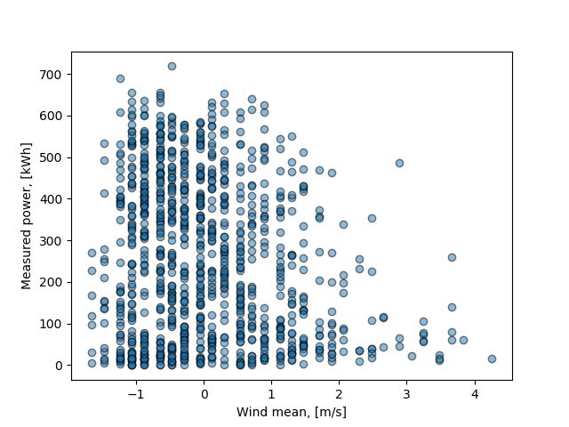
Abstract                Abstrakt
In my thesis, I have explored essential            V rámci své bakalářské práce, jsem pře-
aspects of the solar power forecasting. I          zkoumal důležité aspekty předpovědi slu-
have reviewed several publickly available          neční energie, několika bezplatných zdrojů
sources of data and services which are             dat nutných či užitečných pro tuto před-
useful or necessary for the forecast. Fur-         poved’. Také jsem vytvořil dva demon-
thermore, I created two demonstrations             strativní modely předpovědi, které byly
of the forecasting models that both rep-           založené na různých technologiích. První
resent different approaches for the solar          model byl postaven na předpovědi sluneč-
power forecast. The first model was based          ního záření a oblačnosti. Druhý model byl
on the Sun irradiation and cloudiness fore-        založen na historických datech. Druhý mo-
cast, whereas the second model was built           del se prokázal jako lepší a dosáhl řady
on the historical data. The second model           přesnosti rovné koeficientu determinace
was more precise than first, and achieved          0.89 a hodnoty absolutní chyby 47.465
the range of performance equal to 0.89             kW h, když střední hodnota byla stano-
of The Coefficient of Determination and            vená 256 kW h.
47.465 kW h of the Mean Absolute Error,
whereas the mean value of the power ob-            Klíčová slova: Předpověd’ výkonu
servations is 258 kW h.                            solárního panelu, Data pro předpověd’
                                                   výkonu solárního panelu, SVM regrese
Keywords: Solar panel power forecast,
Data for solar plant power forecast, SVM           Překlad názvu: Predikce výkonu
regression                                         fotovoltaické elektrárny z předpovědi
                                                   počasí
Supervisor:   Ing. Martin Schaefer

                                              vi
Contents
1 Introduction                                  1
1.1 Structure of the thesis . . . . . . . . . . 2
2 Background theory                                    3
2.1 White-box forecasts . . . . . . . . . . . .        5
 2.1.1 Environment parameters . . . . .                5
 2.1.2 Panel parameters . . . . . . . . . . .          6
2.2 Black-box forecasts . . . . . . . . . . . .        7
3 Sources of data                                      9
4 Implementation of the white box
model                                                   11
4.1 Model . . . . . . . . . . . . . . . . . . . . . . . 11
4.2 Quality of the prediction . . . . . . . 14
5 Implementation of the black box
model                                                   17
5.1 Model . . . . . . . . . . . . . . . . . . . . . . . 17
5.2 Quality of the prediction . . . . . . . 21
6 Conclusion                                          25
Bibliography                                          27
A Graphs                                              29

                                                             vii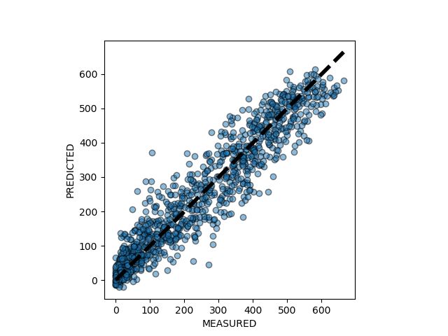
Figures                    Tables
2.1 Distribution of forecasting methods                           3.1 Comparison between online
 in studies by type (source: [1]) . . . . 4                        services and by their provided
2.2 Forecasting scheme of a white-box                              parameters. . . . . . . . . . . . . . . . . . . . . 10
 model (source: [16], 2009, © IEEE) 6
2.3 Cross-validation scheme. At each                              4.1 Example of a response to the
 iteration of the algorithm, testing                               request. The Sun azimuth and
 fold is held out to evaluate the final                            altitude angles (hours before sunrise
 performance, if the evaluation on the                             and after sunset excluded). . . . . . . . 13
 validation subset is succeed. . . . . . . . 8

4.1 Comparison of power predicted by
 the "Forkast" and my white-box
 model for two days. . . . . . . . . . . . . . 14
4.2 The Sun angles dependencies and
 the "Forkast" prediction. . . . . . . . . . 15

5.1 Different kernels, the illustrative
 example (source: [11], http://
 scikit-learn.org/stable/auto_
 examples/svm/plot_iris.html). . 18
5.2 Sun irradiation and mean
 temperature to measured power
 values scatter plots. . . . . . . . . . . . . . 20
5.3 The black-model regression
 example over 100 randomly picked
 days (sorted by the absolute value of
 the measured power).
 C = 1000, γ = 0.01. Prediction score
 R2 = 0.89. . . . . . . . . . . . . . . . . . . . . . 21
5.4 Normalized histogram of absolute
 error (top) (integral over the y-axis
 (density) is 1) in the testing subset
 and measured and predicted values
 scatter plot (bottom). . . . . . . . . . . . 22

A.1 Mean wind speed to measured
 power values scatter plot. . . . . . . . .         29
A.2 Minimal temperature and
 maximum temperature to measured
 power values scatter plots. . . . . . . .          30
A.3 Mean pressure and humidity to
 measured power values scatter plots.               31
A.4 Snow height to measured power
 values scatter plot. . . . . . . . . . . . . . .   32

                                                           viii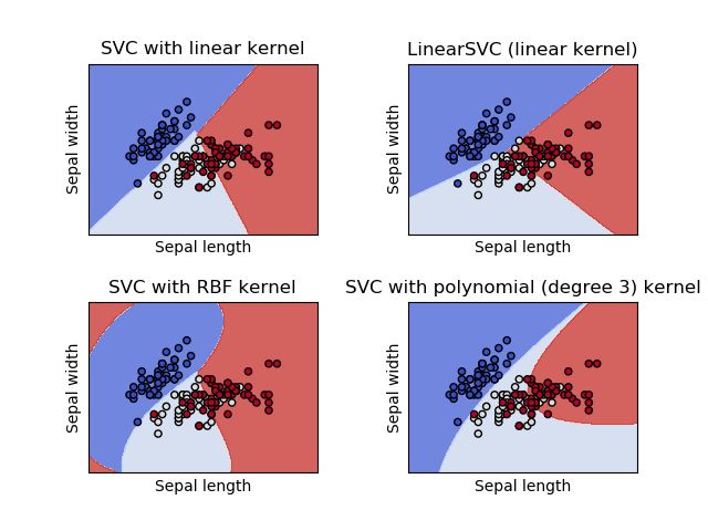
Chapter        1
     Introduction

Choice of my bachelor thesis was mainly inspired by the increasing role of the
photovoltaic systems in overall energy consumption (growing at more than
twice the rate of demand: +4.7% [14]). Ecological and rapidly developing
power characteristics of PV systems motivate researches from around the
world to explore this field. But unfortunately, by now there are no such
widely affordable solar systems that can fully replace any other sources of
energy in complex energy grids (e.g. coal, gas, oil). Despite this, we have an
opportunity to partly replace non-renewable sources of energy in complex
electrical grids by integrating a solar power plant. After doing this, the power
engineer should know how much his energy system should rely on the solar
power. This amount of energy or at least its forecast should be known in
order to plan consumption of energy and to keep energy loads consistent. As
we can see from the research [15], combining wind and solar energy sources
in a distribution system could cause voltage rise and overloading of system
components. Nevertheless, if all circumstances that could cause these defects
are reduced to their minimum, introduction of PV plant could noticeably
reduce losses within the system. For this and other purposes exists the solar
power forecast, that predicts the value of power intake of the solar plants.
   Based on this conclusion, I decided to bring a modest contribution to the
field of the PV power forecast. I explored online sources for the subject of
reliable data needed for the forecast. These data will help building my own
prediction models, and they are accessible for everyone who has a computer
with the Internet connection and a solar power plant. My foremost attempt
at writing this thesis was the simplicity and reusability of the approaches
that will help to reuse them for further researches.
   On the other hand, such aspects as the underlying principle of solar cells
functioning, either electrical or physical, various technologies of cells, features
selection concepts, selection of the model classifier that is required for good
statistic model work and its’ working principle are not in the scope of this
thesis. For these topics and further information may me refer a reader to
such authors as: Arno Smets, Klaus Jäger, Olindo Isabella, Miro Zeman,
René van Swaaij [6] (the solar technology field), Shai Shalev-Shwartz and
Shai Ben-David [7], Stephen Marsland, [8] (the machine learning field).

                                        1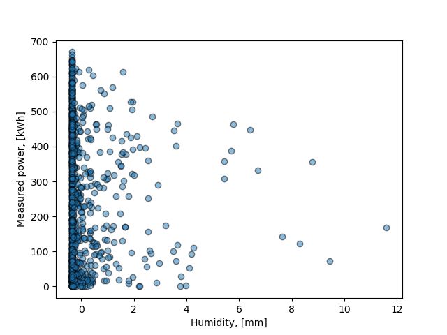
1. Introduction   .....................................
    1.1     Structure of the thesis

Now let me present the structure of this thesis. The Chapter 2 guides
a reader through the background theory of the solar power forecasting,
including forecast techniques that are based on the PV plant configuration,
mounting, inside technology (so-called "white-box" systems) and forecasts
based on statistic data computations (so-called "black-box" systems). Both
of these forecasting techniques types use weather data as an input. The
Chapter 3 reviews sources of data (including statistical) and services, that are
required for functioning of mentioned above models. Following two chapters,
Chapter 4 and Chapter 5, show my implementation of both demonstrators of
the forecasting models for the medium range hourly and daily power forecasts
with the explanation of their work principles, used data, and discussion about
the quality of their prediction. The final Chapter 6 recapitulates and discuss
all the work that was done in my thesis.

                                       2
Chapter 2
Background theory
There is a relatively big number of forecasting techniques that are found to be
useful in various applications, such as economics and energetic. For example,
to predict what volume of energy will be produced by solar plants in the
whole country for a year and compute the price for electricity, to predict how
much energy will be generated daily by a power solar plant in the range of
one week [18], or to predict what amount of energy will produce a small-scale
grid-connected solar plant on a roof in the next hour [19]. All mentioned above
examples show us that the categorization between models may be presented
in a range of the prediction – "forecast horizon", intervals of the prediction
– "forecast resolution" and a number of solar panels that will be included
in a prediction: will it be a single panel, solar power plant or a multiple
power plants. Moreover, there is an opportunity to divide these models even
more, by their implementation – into three main groups. In the first group,
white-box models are models based on the solar irradiation forecasts which
may be obtained from various Numerical Weather Prediction models (NWP
in the further reading), what can as well be the biggest source of uncertainty
of these models, and on a solar plant implementation and technology. The
second group consequently is black-box models, which includes models that
are based on regression methods and statistics, built on obtained historical
data about PV plant power and criteria (or features) that are correlated with
the power this solar power plant produce. Accordingly, the third group, grey-
box models is the group which models are based on the particular combination
of different black-box and white-box methods in a specific way. This model
can be blended with models of either the same type: black-box, white-box by
itself (e.g.: Random Forests classification for clustering of samples into groups
+ SVM regression for predicting the power output – both are black-box
approaches), or different types: black-box + white-box. In the latest research
on the subject of different photovoltaic techniques, the distribution of each
method in studies was discovered in [1], and according to the information
introduced in Figure 2.1, statistical methods appear to be the most chosen
for solar panels forecasting (primarily Artificial Neural Networks, Support
Vector Machines, and Regressive methods [1]).
32. Background theory ..................................
Figure 2.1: Distribution of forecasting methods in studies by type (source: [1])
Since there is a huge number of methods and approaches that can be used
for specific tasks, model developers encountered the need to compare them in
order to select models that have better performance than other. Models are
compared on accuracy by introducing and applying statistical metrics, such
as Normalised Error, Mean Absolute Error, Standard Deviation of Errors,
Root Mean Square Errors, Pearson’s coefficient etc. Furthermore, other
forecast circumstances must be recognized when the quality of the prediction
is evaluated, including, according to [1]: Climatic variability, Day/night
values and normalization, Sample and spatial aggregation, Testing period and
Specific plant attributes, – because they can significantly affect the quality of
prediction, and at the same time are still useful for particular tasks.
To summarize all mentioned above, let me introduce the List 2 that guides
..
the reader and help to develop his very own prediction model:
. Establish the goal of a prediction.
1. What value the algorithm will aim to reach?
2. What is the required forecast horizon, resolution?
3. What is the amount of panels?
.
..4. What are the forecast circumstances?
Implement the model.
1. Choose the model type (black-box, white-box, gray-box).
2. Gather required data.
.
.3. Filter data and tune tools of the model if needed.
Evaluate the model quality.
1. Choose the optimal accuracy criteria.
2. Choose the best model based on the accuracy criteria.
4................................. 2.1. White-box forecasts
Following this scheme, the reader will be able to develop his own forecast
model. According to it, I created my own white-box and black-box forecasting
systems described in Chapter 4 and Chapter 5. Following sections in the
current chapter covers both black-box and white-box model main principles.
2.1 White-box forecasts
White-box models are models that are based on the solar irradiation forecasts
and on the solar plant implementation and technology. A good place to start
describing white-box forecasting models is to highlight significant aspects
that lay the foundation for its’ development. Firstly, I describe parameters
of the environment that are crucial for the prediction itself. Then, I dis-
cuss parameters that are in connection with solar plant orientation and its’
characteristics.
2.1.1 Environment parameters
Entirely logical, that two main parameters of the environment that determine
PV system behavior are the cloud cover ratio above the plant surface and the
amount of extraterrestrial sun irradiation – but not only them. In the addition,
there are several particular parameters that should also be considered in order
to achieve more precise model, including a temperature at the ground level,
the panel itself, wind temperature, speed and direction, the moisture of the air,
snow cover thickness etc., that also have the nonzero impact on the prediction
and therefore are placed in the field of advanced forecasting techniques. For
simplicity, all mentioned above criteria can be reduced to just two of them
in the Chapter 4: extraterrestrial sun irradiation and cloud cover. For more
deep analysis of the impact of particular parameters, let me refer a reader to
[6].
There are several components of the solar irradiation, according to [2]:
Direct Normal Irradiance (DN I), Global Horizontal Irradiance (GHI), and
Diffuse Horizontal Irradiance (DHI). The relation between them may be
shown in the Equation 2.1 [2]:
GHI = DHI + DN I · cos(θ), (2.1)
where(θ is the solar zenith angle. In the field of solar power forecast, we
are interested in the value of the global horizontal irradiance. This value
can be obtained by requesting one of NWP models. Categorization of these
models can be made by the type of predicted irradiation they may provide:
"clear sky" models or extraterrestrial irradiance models. "Clear sky" means,
that these models compute the value of irradiation that reaches the specified
area at the ground level with consideration to the atmosphere condition (air
turbidity) and the level of cloudiness. The second type of models simply
computes irradiance as the product of the solar constant (I0 = 1360 W/m2)
and cosine of the Sun zenith angle in a certain time as it described by the
Equation 2.2 [2].
52. Background theory ..................................
ItEX = I0 · cos(θt ), (2.2)
The cloud cover parameter is typically arranged into layers: high, middle
and low levels, and is the second crucial parameter for the solar power
forecasting, because it directly affects the amount of irradiation that can be
diffused in clouds.
2.1.2 Panel parameters
After parameters of the environment, I describe parameters of a solar plant
orientation. Concerning solar panel orientation and its characteristics, most
of the effect on the result of the prediction is made by a mutual orientation of
the Sun and the considered solar panel. Since that, and the fact, that inside
panels’ characteristics are oftentimes difficult to measure, for simplicity I
selected just two parameters for calculation in the Chapter 4: panel’s tilt and
azimuth angles. Once more, in the section of white-box forecast systems is a
great number of different modeling techniques that are made for various tasks,
hence one should choose carefully not to dismiss any valuable parameter that
could increase the system accuracy.
To recapitulate this section, let me offer for viewing the forecasting scheme
of the PV power, presented in Figure 2.2:
Figure 2.2: Forecasting scheme of a white-box model (source: [16], 2009, © IEEE)
Since we completed the review of essential parameters needed for the white-
box forecast and briefly explored these models’ developing algorithm in List
2, the next chapter discusses same items for black-box models.
6................................. 2.2. Black-box forecasts
2.2 Black-box forecasts
Black-box models (or statistical) are built on historical datasets and represent
the statistic approach to solve the problem of power prediction in PV systems.
This group of models is frequently split into two other groups (or three, if
we talk about hybrid methods [1]): such that are based on the Artificial
intelligence techniques, or autoregressive methods. Whereas according to
Figure 2.1, Artificial Neural Networks is the most popular technique in the
solar power forecasting, there are less popular but still powerful methods
as k-Nearest Neighbors, Support Vector Machines and Random Forests,
other regressive methods. Besides, if several methods are combined in the
calculation of the prediction, some studies show that a prediction achieve
even higher accuracy. For example, in [17], based on the ANN-models forecast
proved, that first classifying days into specific groups (e.g. sunny/partly
cloudy/overcast days) before applying regression makes notable improvement
in the accuracy (eg. up to the 1.42 of the Mean Absolute Percentage Error
and the coefficient of determination 0.9997). Because of this, the developer
has a truly wide variety of methods and tools that could be applied in order
to solve any possible specific tasks. Since methods used in black-box models
are based on statistical considerations and approaches, if one considers using
any of these models, there must be a non-zero sample correlation coefficient
between features (or predictors), that he or she selected for model training,
and the measured value. This coefficient is defined by the Equation 2.3.
Furthermore, if classification methods are used, there must be a possibility
to classify training set’s values.
n
(xi − x)(yi − y)
P
i=1
r=s s , (2.3)
n n
(xi − x)2 (yi − y)2
P P
i=1 i=1
where n is the number of samples, xi and yi are single samples of two datasets,
x and y are samples mean.
Moreover, statistical methods often require the number of samples to be
significantly bigger than a number of features – so the developer should pay
attention to this fact. The next important aspect that should be thought
in this field is the features selection and the consistency of data, that one’s
model will be fed. Along with inside parameters and configuration of used
statistic tools, it all can also be changed what can affect the performance
of the model dramatically. Nevertheless, the main advantage of using these
methods is that a programmer does not necessarily need to understand
the deep underlying principles of the configuration of the forecasted PV
system (what its orientation and how the whole system works). Instead,
the developer should have enough understanding in the area of Artificial
Intelligence methods and the nature of the data he uses in the process of
development. And then, therefore, despite this lack of knowledge of physical
processes behind solar systems, he can yet create very robust and precise
72. Background theory ..................................
model that will predict a solar plant power with required accuracy.
However, there are specific problems connected with the field of Artificial
Intelligence methods. The biggest problem of statistic regression models is
that they tend to overfit on the testing samples if the training procedure is not
processed right – after splitting the dataset into training and testing sets (or
into training, testing and validating sets in case of artificial neural networks)
and then applying a cross-validation algorithm for setting of hyper-parameters
(inside parameters of classifier that describes its behavior) and gathering the
information about the uncertainty of the prediction. Figure 2.3 summarily
shows how the procedure of cross-validation is computed:
Testing fold Training folds
Validation Training
Figure 2.3: Cross-validation scheme. At each iteration of the algorithm, testing
fold is held out to evaluate the final performance, if the evaluation on the
validation subset is succeed.
To create a before-mentioned model, whereas one is choosing between the
different approaches, it should be noted that they have their own advantages
and disadvantages, and very frequently one method is preferable than another
(e.g. if there is a great amount of features and a smaller amount of samples in
each category, it is often preferable to choose methods as Naive Bayes because
of their high calculation speed, whereas such methods as SVM are slower).
For covering this part of the theory, as well as preprocessing of data, let me
offer the reader these resources that imply knowledge of Python programming
language: [11], [9]. In addition, let me introduce the Python library, that
certainly will help the reader to visualize and manipulate with data: [12].
8Chapter 3
Sources of data
In this chapter, I introduce common sources of publicly available data and
services and their characteristics for the solar panel power forecasting, based
on a weather forecast given that black-box and white-box essential aspects
have been reviewed. Firstly, I list and benchmark free APIs, datasets and web-
services, that provide free data for developing white-box models. After this
been made, in the left text I append information about available statistic data
needed for black-box models. On the basis of judgment, that I made in the
previous Chapter 2, for a proper white-box modeling of solar power predictor
it is crucial to be able to gather data about cloudiness, the Sun irradiation
that reaches atmosphere and solar panel mounting characteristics. Since
the maximum power of the particular panel (kWp), its placement (latitude
and longitude), its orientation (tilt and azimuth angles) are expected to be
known, we can note, that we are only left to find free services or APIs that
offer the information about future location-specific cloudiness and the Sun
irradiation (their forecast). The following List 3 of services and APIs shows
related sources of data for white-box and black-box forecasting:
. https://openweathermap.org/ (5 days/3 hour forecast API, Weather
maps API, max. 60 calls per minute)
. https://darksky.net/dev/docs#forecast-request (7 days/1 hour
forecast, max. 1000 calls per day)
. https://www.wunderground.com/weather/api (10 days/1 hour fore-
cast, 10 calls per minute)
. https://developer.worldweatheronline.com/api/ (15 days/1 hour
interval, not for free)
. https://developer.accuweather.com/packages (5 days/ 1 day fore-
cast, 50 calls per day)
. https://www.apixu.com/ (7 days/1 day forecast, 10000 calls per month)
Following Table 3.1 shows whether mentioned-above services provide data
that is relevant for modeling white-box system (Global Solar Irradiation
[W/m2 ], Temperature of air [C ◦ ], Wind Speed at ≈ 10 m [m/s], Cloud cover
[%], Pressure [P a]):
93. Sources of data ....................................
Table 3.1: Comparison between online services and by their provided parameters.
Weather Service Sun irr Temp Wind Sp Clouds Press
OpenWeatherMap No Yes Yes Yes Yes
Darksky Yes Yes Yes Yes Yes
Wunderground No Yes Yes Yes Yes
Worldweatheronline Yes Yes Yes Yes Yes
Accuweather Yes Yes Yes Yes Yes
Apixu No Yes No Yes No
In addition, there are other services that are able to bring highly-correlated
information about the Sun Irradiation that can substitute the absence of
the Sun Irradiation forecast value. Such services that provide azimuth and
altitude angles of the Sun during the day (e.g. http://aa.usno.navy.mil/
data/docs/AltAz.php, https://www.suncalc.org/).
There are as well such high-level online services that give you the pre-
dicted power directly: https://www.solarserver.com/service/, https:
//forkast-renewables.com/. But their full function is not for free and it
is not transparent what is the principle of their work. I used the "Forkast"
white-box prediction model as the benchmark for my own white-box model.
Nevertheless, if the reader prefers to deal with more precise and complex
forecast responses or to develop Black-box forecasting model, there is an oppor-
tunity to obtain these data in form of a grid-scale location forecast or historical
dataset, which probably requires installing some of the decoding utilities (more
about decoding utility reader can read on this web-page: https://software.
ecmwf.int/wiki/display/CKB/How+to+read+or+decode+a+GRIB+file).
Since this fact, developer will probably need to use one of NWP models
functionality. For this, let me introduce Numerical Weather Prediction models:
http://www.noaa.gov/ (National Oceanic and Atmospheric Administration),
https://www.ecmwf.int/ (European Centre for Medium-Range Weather
Forecasts). These models are used for scientific purposes and provide either
historical or forecast weather data, that are encoded in .grib* or a different
scientific format. One should note, that there are other NWPs that could
be used instead, including NWPs which are local to the area where the
solar panel is placed. Historical data, that was mentioned above, will be
required for black-box models development. Mentioned that, let me present
you the NWP "Aladin" that is local for the Czech Republic: http://portal.
chmi.cz/files/portal/docs/meteo/ov/aladin/. It is provided by Czech
Hydrometeorological Institute.
For now, the reader is informed about various sources of data that are
required for building his very own white-box or black-box prediction model.
In the upcoming Chapter 4, I introduce the simple white-box model that I
built first when have started exploring the field of solar power forecast.
10Chapter 4
Implementation of the white box model
My approach was to introduce a prediction model which would forecast the
power loads that are provided by a single hypothetical PV plant with the
maximum 5-kilowatt peak that is placed in Prague. I chose the forecast horizon
of 3 days ahead and the forecast resolution of 1 hour. Last circumstances of
this forecast are these: the orientation of my virtual solar panel, according to
information presented on this web-page [13], is [45◦ ] tilt and [180◦ ] azimuth
angles, because of the virtual panel placement latitude ( [50◦ ] North) and the
time of year – Spring.
Since the goal was set properly, the following step was to implement the
model.
4.1 Model
As this Chapter 4 name suggests, the model type is white-box. Given the
consideration I made in Chapter 2 about white-box essential parameters, the
amount of energy of a solar panel strongly depends on clouds coverage of sky,
panel orientation on surface in relation with the Sun elevation and azimuth
angles. Considering that, I split the task into two subtasks: firstly, I had to
examine the dependence between the percent of the energy that solar panel
produces and its’ mutual orientation with the Sun, and secondly, to combine
this amount of energy with information about forecasted cloud coverage. To
calculate the percent of the energy that outcomes from the Sun angles and
panel orientation I needed to use the Equation 4.1 that was introduced in [6],
that is valid for latitudes 50 − 60◦ N, and the Sun elevation angle more than
0◦ with additional restriction that the difference between the panel’s and the
Sun’s azimuths is less than 90◦ :
Gbeam
= (sin(β)cos(α)cos(Am − As ) + cos(β)sin(α)), (4.1)
Gdirect
where Gbeam and Gdirect are the beam and the direct Sun radiations on
the panel, β and α are the panel’s tilt and the Sun’s elevation angles, Am
and As are the panel’s and the Sun’s azimuth angles respectively. After
the first part of the task was completed, it was necessary to multiply value
calculated in the equation mentioned above by the coefficient that is equal
114. Implementation of the white box model .........................
to (1 − clouds_coef ), where clouds_coef is the value equals to forecasted
percent of the sky is covered by clouds. After this was made, is was possible
to get the model output by multiplying calculated value by maximum panel
load, which in my case was 5 kWp. Proceeding from the fact, that this model
requires inputs (the Sun angles and cloudiness), next part of this section
describes data that I used to implement this model.
According to the mentioned above requirement, I was looking for an open
reliable source of weather data that could allow me to intake relatively precise
information about the weather (mainly cloud coverage) for at least 3 days
with 1-hour intervals. After a research, I found out that there are several APIs
for weather application developers that offer different forecasts, from which I
chose API that offers Wunderground, because it had 10 days forecast option
with 1h. interval, almost all required parameters and the good documentation
including examples of API calls written in the Python programming language,
which I used for writing my project.
Particularly, I used API call "hourly10day" and "astronomy" which gave
me necessary information in .json format, that is well documented on the
web-page: https://www.wunderground.com/weather/api/d/docs. As an
example of this response I introduce a small piece of response field:
{
"hourly_forecast": [
{
"FCTTIME": {
...
"isdst": "0",
"mday": "11",
"mday_padded": "11",
"min": "00",
"min_unpadded": "0",
"mon": "2",
"mon_abbrev": "Feb",
"mon_padded": "02",
"month_name": "February",
"month_name_abbrev": "Feb",
"pretty": "7:00 PM CET on February 11, 2018",
...
},
...
"sky": "88",
}
]
...
}
12...................................... 4.1. Model
Next, it was necessary for the prediction to gather the information about
the Sun’s movement during the day. For this purpose, I used the web-page
of the Astronomical Applications Department of the U.S. Naval Observa-
tory. Namely http://aa.usno.navy.mil/data/docs/AltAz.php, to get the
Sun’s altitude and azimuth angles. As a reply for the request, it gives user
information presented in the text form on HTTP-page. There is an example
of this reply presented in the Table 4.1.
Table 4.1: Example of a response to the request. The Sun azimuth and altitude
angles (hours before sunrise and after sunset excluded).
Time, [h] Altitude angle, [C ◦ ] Azimuth angle, [C ◦ ]
07:00 -4.7 107.9
08:00 4.3 119.4
09:00 12.1 131.7
10:00 18.4 145.2
11:00 22.9 159.9
12:00 24.9 175.6
13:00 24.3 191.5
14:00 21.2 206.9
15:00 15.8 221.1
16:00 8.8 234.0
17:00 0.8 246.0
18:00 -8.7 257.3
After my model began to function, it remained for me to evaluate the
quality of its prediction.
134. Implementation of the white box model .........................
4.2 Quality of the prediction
To evaluate the quality of the prediction, I chose this service as a benchmark:
https://forkast-renewables.com/home, since I failed to gather real power
data at the moment of creation of this model to evaluate it in a proper way.
"Forkast" is the free web-service that provides energy production forecast and
consumption management tools.
Figure 4.1: Comparison of power predicted by the "Forkast" and my white-box
model for two days.
14............................... 4.2. Quality of the prediction
As it can be seen from Figure 4.1, my model returns completely different
predicted values to compare with Forkast service’s output values, which can
be caused by different weights of input parameters, and most possibly by
different forecast resources that are used to gather weather data. I made this
conclusion, because by reducing the cloudiness parameter for the first testing
day, I obtained the Figure 4.2 with the shape that repeats the "Forkast"
predicted values with an offset ≈ 2 kW .
Power forecast for 2018-02-14
5
Angle relation
Forkast
4
3
power (kW)
2
1
0
8 10 12 14 16 18
time (hours)
Figure 4.2: The Sun angles dependencies and the "Forkast" prediction.
Despite this, it does not mean that it is not working properly. For further
evaluation and tuning, there is a need for real data from real solar panels
with the information about their configuration and mounting parameters.
Nevertheless, the model itself can be used as a tool for a basic analysis. More
deep approach will be required in order to maintain sufficient accuracy level
necessary for commercial needs.
1516
Chapter        5
     Implementation of the black box model

My next model aimed to forecast energy accumulated daily by the real PV
plant which is mounted on the CTU in Prague FEE building. I chose the
forecast horizon of 10 days ahead and the forecast resolution of 1 day. The
range and horizon of the forecast was selected due to the existence of the
research based on the SVM regression made by researches from Italy [5]. As
a part of the research, they obtained the Median Absolute Percentage Error
below 12% when were using NWP models. I partly replicated their method-
ology of developing the forecasting model, when was selecting parameters of
estimator by applying a grid search, and was consulting their observations
when was choosing the accuracy metrics.
   Following the goal was set, the latter step was made to implement the
model.

     5.1    Model

After considering gaps that were made in the previous Chapter 4, I chose
to operate with real data, so that the accuracy of the prediction could
be measured. For selecting the model estimator type, I pointed to these
researchers: [1], [3], [4], [5], and chose the SVM Regression approach as one of
the most popular and simple to implement due to the available code libraries
and detailed documentation.
   The Support Vector Machine method nowadays is actively used in the
field of machine learning for such tasks as regression, outliers detection and
classification. The basis of this method underlies in the two main principles:

 .   the linear classification that divides features into two subplanes via
     hyperplane leading by the maximizing of the minimum distance between
     hyperplane and samples of different categories (this distance is called
     "margin")

 .   the "kernel trick" that allows using SVM method for non-linear problem
     solving by conversion of the non-linear-separable problem into the linear-
     separable with use of a kernel transformation of features to a higher
     dimension transformed features space.

                                      17
5. Implementation of the black box model .........................
Further, regression analysis is implemented via minimization of the loss
function (that maps margin to the "cost" value of it), which has explicit
tolerance cost.
Despite all the variety of SVM configurations, for choosing estimator param-
eters of my model I only set for tuning most crucial of them. These are C and γ
hyper-parameters (as it is described in http://scikit-learn.org/stable/
auto_examples/svm/plot_rbf_parameters.html [11]: "the gamma param-
eter defines how far the influence of a single training example reaches, with
low values meaning ‘far’ and high values meaning ‘close’.", and "The C pa-
rameter trades off misclassification of training examples against simplicity of
the decision surface") and type of kernel.
In the first place, most importantly, I selected the Radial basis function
kernel, because it allows SVM to choose more curved shapes of hyperplanes
than others and I had the very noisy and diverse set of data. The illustrative
example of how different kernels work can be seen in Figure 5.1 [11].
Figure 5.1: Different kernels, the illustrative example (source: [11], http:
//scikit-learn.org/stable/auto_examples/svm/plot_iris.html).
18...................................... 5.1. Model
After the kernel was selected, as the next step I decided not to choose
C and γ parameters directly, but include this selection as the part of
my model’s code as it is described in http://scikit-learn.org/stable/
modules/grid_search.html – with use of the cross-validation k-folds tech-
nique on a list of hyper-parameters’ values that I decided to give to my model:
γ: 0.1, 0.01, 0.001, and C: 10, 100, 1000. As the metric for this selection, I
chose the coefficient of determination (which "provides a measure of how well
future samples are likely to be predicted by the model" [11]). According to
[11], if ŷi is the predicted value of the i-th sample and yi is the corresponding
true value, y is the mean, then the score R2 estimated over n is defined as in
the Equation 5.1.
n−1
(yi − yˆi )2
P
2 i=0
R (y, ŷ) = 1 − n−1
, (5.1)
(yi − y)2
P
i=0
Given that, my model was ready for use and the next step that I would
like to describe to a reader was my further work with training and testing
data preprocessing.
Following my request to the Laboratory of Photovoltaic Systems Diagnos-
tics of CTU for the historical daily data about the power that solar plant
accumulates, I obtained the data for slightly more than 7 years. After think-
ing about advantages and disadvantages of different weather data sources, I
decided to use Czech Hydrometeorological Institute daily observations his-
torical database, because it contained most relevant to the Sun irradiation
data for the specific location (e.g. "daily sun day duration") and was simple
to work with because of the .csv format. After this was made, both solar
power and weather historical datasets were obtained. Following to previous
steps, I proceed to the data preprocessing, which included broken samples
deleting from the dataset, followed by shuffling of the rest of samples and
splitting them into training and testing subsets. After this was made, I left
with fitting and predicting process. A reader can see most relevant results
which I received by formatting the data in Figure 5.2. The rest of data can
be seen at Appendix A at Figure A.1, Figure A.2, Figure A.3, Figure A.4 in
form of scatter plots of measured power values (labels), and scaled weather
data (features) values.
195. Implementation of the black box model .........................
Figure 5.2: Sun irradiation and mean temperature to measured power values
scatter plots.
As it can be seen from scatter plots, there is a big amount of outliers. But
nevertheless, I decided to keep this datasets unmodified, because SVM might
find all samples useful, although this will prolong the calculation time.
20............................... 5.2. Quality of the prediction
5.2 Quality of the prediction
The last part of the model development process was the evaluation of the
prediction quality. To estimate my model precision and examine its per-
formance, as the metrics I chose the mean absolute error with the unit of
measure kWh and the coefficient of determination (the R2 score), because
the Median Absolute Percentage Error showed too high value (≈ 37%) and
therefore was not used. This was probably caused by the absolute error, that
is same for big and small power values. Which means, that the percentage
error is much bigger for small values. The mean absolute error is defined in
the Equation 5.2.
n−1
M AE(y, ŷ) = n−1
X
|yi − ŷi |, (5.2)
i=0
where n is the number of samples, ŷi is the predicted value of the i-th sample.
After this was made, I entered samples from the testing subset of data
to ascertain the accuracy value. My model showed the performance equal
to 0.89 coefficient of determination and 47.465 kW h mean absolute error
whereas the mean value of all power measurements is equal to 258 kW h. The
example of this regression sorted by the absolute value of the measured power
can be seen in Figure 5.3.
Figure 5.3: The black-model regression example over 100 randomly picked days
(sorted by the absolute value of the measured power). C = 1000, γ = 0.01.
Prediction score R2 = 0.89.
215. Implementation of the black box model .........................
As it can be seen from the regression example Figure 5.3, my model makes
bigger percentage errors when predicting small values of the power outcome,
which explains the fact, that the Median Absolute Percentage Error was too
big. The following normalized histogram of absolute error and scatter plot on
Figure 5.4 will demonstrate the distribution of the absolute error of prediction
probability in the testing subset and scatter plot of measured and predicted
power values to the reader.
Figure 5.4: Normalized histogram of absolute error (top) (integral over the
y-axis (density) is 1) in the testing subset and measured and predicted values
scatter plot (bottom).
22............................... 5.2. Quality of the prediction
As it can be seen from the histogram, the great part of all errors made by
my model are placed at the range 50-125 kW h. Bearing in mind the mean
value of all power measurements, that is equal to 258 kW h, I can state that
the accuracy of my model is far from perfect. Following the histogram there
is an illustrative scatter plot that shows the reader how far are the predicted
values (blue dots) distanced from the real values (black interrupted line).
2324
Chapter        6
    Conclusion

After the all work that was done on this project, I would like to summarize the
content of my thesis, comment the results and discuss possible improvements.
At the first place, I presented the topic of the solar power forecasting to the
reader, provided the expeditious course to the basic concepts of this field. It
included classification of forecasting approaches, review both of black-box and
white-box models and their main dependencies, advantages and disadvantages.
After this was made, I listed sources of data that a developer of a prediction
model will presumably need and made the brief comparison review, I also
mentioned indirect sources of information that can also be handy for the
developer, and described NWP models.
   Furthermore, I developed the white-box model that unfortunately I was not
able to evaluate due the absence of real data, and therefore it was not appro-
priate for any commercial or precise prediction use. The methodology of the
model development can be used as the basis for other PV forecasting models
though, because of its’ function simplicity and importance of the parameters
of the Sun angles and cloudiness used for this approach. But one should note,
that it does not imply weight setting for particular parameters, which should
be implemented in order to obtain precise values of the prediction.
   Following the white-box model, I made the black-box model that reached
the 0.89 of the coefficient of determination on the given data. Since outliers
were not detected and removed from the data, I propose that my model
has nearly "90% of accuracy of the prediction" on condition of "zero forecast
uncertainty", because the data of the training and testing subsets were
measured, but not forecasted. My model can be used, after reconfiguration,
as the basic prediction model for personal use, as well as the component of
a free web-application for predicting a power that is produced daily by any
solar plant that is placed in Prague. For this, this plant has to provide data
about measured power during the day for the extended period of time. But
it is not yet possible to use it for commercial use, because the prediction is
still far from perfect. The deeper research should be made in the features
selection process, consistence of datasets that are provided and measured by
sensors that put their own uncertainty into the measurement process, as well
as the selection of the more appropriate for this problem machine learning
algorithm.

                                      25
6. Conclusion ......................................
As the direction of the future work on this topic, I see the use of real data
for evaluation of the white-box model performance and more penetrating
analysis of physical processes and dependencies that exist in this field. I also
suggest the use of forecasted weather for the black-box model performance
evaluation and estimating the minimal length of the training subset that will
be sufficient for achieving the optimal performance, as well as the selection of
the machine learning approach that can be more appropriate for this problem.
26Bibliography
[1] Review of photovoltaic power forecasting, J. Antonanzas, N. Osorio, R.
Escobar, R. Urraca, F.J. Martinez-de-Pison, F. Antonanzas-Torres, Pub-
lication: Solar Energy. Publisher: Elsevier, Date: 15 October 2016
[2] Solar forecasting methods for renewable energy integration, Rich H. Inman,
Hugo T.C. Pedro, Carlos F.M. Coimbra. Publication: Progress in Energy
and Combustion Science, Publisher: Elsevier, Date: December 2013
[3] A benchmark of statistical regression methods for short-term forecasting
of photovoltaic electricity production, part I: Deterministic forecast of
hourly production, M. Zamo, O. Mestre, P. Arbogast, O. Pannekoucke,
Publication: Solar Energy, Publisher: Elsevier, Date: July 2014
[4] A benchmark of statistical regression methods for short-term forecasting
of photovoltaic electricity production. Part II: Probabilistic forecast of
daily production, M. Zamo, O. Mestre, P. Arbogast, O. Pannekoucke.
Publication: Solar Energy, Publisher: Elsevier, Date: July 2014
[5] Short-term predictability of photovoltaic production over Italy, Matteo De
Felice, Marcello Petitta, Paolo M. Ruti. Publication: Renewable Energy,
Publisher: Elsevier, Date: August 2015
[6] Solar Energy: The Physics and Engineering of Photovoltaic Conversion,
Technologies and Systems, Olindo Isabella; Klaus Jäger; Arno Smets; René
van Swaaij; Miro Zeman. Publisher: UIT Cambridge Ltd., 2016
[7] Understanding Machine Learning: From Theory to Algorithms,
Shai Shalev-Shwartz and Shai Ben-David, Publisher: Cambridge
University Press, 2014; http://www.cs.huji.ac.il/~shais/
UnderstandingMachineLearning/ [Online; accessed 2018-05-22]
[8] Machine Learning (An Algorithmic Perspective), Stephen Marsland. Pub-
lisher: CRC Press, 2015
[9] Building Machine Learning Systems with Python, Willi Richert and Luis
Pedro Coelho. Publisher: Packt Publishing, 2015
27Bibliography ......................................
[10] Learning with Kernels: Support Vector Machines, Regularization, Opti-
mization, and Beyond (Adaptive Computation and Machine Learning),
Bernhard Schölkopf, Alex Smola. Publisher: MIT Press, Cambridge, MA,
2002
[11] Scikit-learn: Machine Learning in Python, Fabian Pedregosa, Gaël Varo-
quaux, Alexandre Gramfort, Vincent Michel, Bertrand Thirion, Olivier
Grisel, Mathieu Blondel, Peter Prettenhofer, Ron Weiss, Vincent Dubourg,
Jake Vanderplas, Alexandre Passos, David Cournapeau, Matthieu Brucher,
Matthieu Perrot, Édouard Duchesnay. Journal of Machine Learning
Research, 12, 2825-2830, 2011. Publisher: http://jmlr.org/papers/
v12/pedregosa11a.html. http://scikit-learn.org/ [Online; accessed
2018-05-22]
[12] SciPy: Open Source Scientific Tools for Python, Jones E, Oliphant
E, Peterson P, et al., 2001-, http://www.scipy.org/ [Online; accessed
2018-05-22].
[13] Optimum Tilt of Solar Panels , Charles R. Landau, http://www.
solarpaneltilt.com/ [Online; accessed 2018-05-22]
[14] REN21. 2017. Renewables 2017 Global Status Report Paris: REN21
Secretariat, 2017
[15] Systems Perspectives on Renewable Power: Challenges of integrating
solar and wind into the electricity grid, David Steen, Joel Goop, Lisa
Göransson, Shemsedin Nursbo, Department of energy and environment,
Publisher: Chalmers University of Technology, 2014
[16] Irradiance Forecasting for the Power Prediction of Grid-Connected Pho-
tovoltaic Systems, E. Lorenz and J. Hurka and D. Heinemann and H. G.
Beyer, Publication: IEEE Journal of Selected Topics in Applied Earth
Observations and Remote Sensing, vol. 2, num. 1, 2009, © IEEE
[17] Short-term forecasting of power production in a large-scale photovoltaic
plant, A. Mellit,A. Massi Pavan,V. Lughi, Publication: Solar Energy,
Publisher: Elsevier, July 2014
[18] Power forecasting of photovoltaic generation, S. H. Oudjana, A. Hellal,
and I. Hadj Mahammed. Publication: World Academy of Science, Engi-
neering and Technology International Journal of Electrical and Computer
Engineering, Vol:7, No:6, 2013
[19] A hybrid model (SARIMA–SVM) for short-term power forecasting of a
small-scale grid-connected photovoltaic plant, Author: M. Bouzerdoum,A.
Mellit,A. Massi Pavan. Publication: Solar Energy, Publisher: Elsevier
Date: December 2013
28Appendix A
Graphs
Figure A.1: Mean wind speed to measured power values scatter plot.
29A. Graphs .......................................
Figure A.2: Minimal temperature and maximum temperature to measured
power values scatter plots.
30....................................... A. Graphs
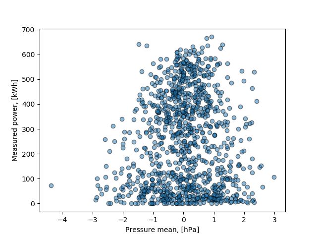
Figure A.3: Mean pressure and humidity to measured power values scatter plots.
31A. Graphs .......................................
Figure A.4: Snow height to measured power values scatter plot.
32You can also read