Carbon monoxide emissions assessment by using satellite and modeling data: Central Mexico case study
←
→
Page content transcription
If your browser does not render page correctly, please read the page content below
Atmósfera 34(2), 157-170 (2021)
https://doi.org/10.20937/ATM.52696

    Carbon monoxide emissions assessment by using satellite and modeling data:
                          Central Mexico case study

          Gilberto MALDONADO-PACHECO1, José Agustín GARCÍA-REYNOSO1*, Wolfgang STREMME1,
    Luis Gerardo RUIZ-SUÁREZ1, José Santos GARCÍA-YEE2, Cathy CLERBAUX3 and Pierre-François COHEUR4

1
  Centro de Ciencias de la Atmósfera, Universidad Nacional Autónoma de México, Circuito Exterior s/n, Ciudad
  Universitaria, 04510 Ciudad de México, México.
2
  Escuela Nacional de Ciencias Biológicas, Instituto Politécnico Nacional, Unidad Profesional Adolfo López Mateos,
  Zacatenco, Av. Wilfrido Massieu 399, Col. Nueva Industrial Vallejo, 07738 Ciudad de México. México.
3
  LATMOS/IPSL, Sorbonne Université, UVSQ, CNRS, Paris, France.
4
  Atmospheric Spectroscopy, Service de Chimie Quantique et Photophysique, Université Libre de Bruxelles, Brussels,
  Belgium.
*Corresponding author; email: agustin@atmosfera.unam.mx

                                     Received: March 15, 2019; accepted: February 18, 2020

                                                               RESUMEN
       En este trabajo se cuantifican y reducen las diferencias de las emisiones en el inventario 2008 respecto a las
       reales mediante el uso de observaciones satelitales y modelación. Se hacen comparaciones de columna de
       monóxido de carbono de los datos satelitales del Interferómetro de Sondeo Atmosférico Infrarrojo (IASI, por
       sus siglas en inglés) contra columnas obtenidas del modelo WRF-Chem, durante febrero de 2011. El análisis
       se realiza a la hora local del paso satelital (10:00 a.m., aproximadamente) sobre la Ciudad de México. Se
       empleó el inventario nacional de emisiones 2008 generado por la Secretaría del Medio Ambiente y Recursos
       Naturales. Se utilizó un método de inversión con los datos de columna del modelo y observados; con ello
       se obtuvieron factores de escalamiento para cinco regiones y la concentración proveniente de las fronteras
       del dominio del modelo, los cuales se emplearon para actualizar las emisiones. Estas emisiones actualizadas
       se usaron en la modelación y el resultado se comparó contra mediciones en superficie. Para la Ciudad de
       México y el Área Metropolitana se obtuvo un factor de escalamiento igual a 0.43 al emplear el Inventario
       Nacional de Emisiones 2008; para Toluca, Morelos y Puebla se estimó un factor menor a uno, mientras que
       para Hidalgo y la concentración proveniente de las fronteras del modelo fue cercano a dos. El desempeño
       del modelo mejoró al incrementar el índice de concordancia y disminuir el error cuadrático medio cuando
       se utilizaron las emisiones actualizadas de CO.

                                                              ABSTRACT
       This paper quantifies and reduces the differences in emissions from the 2008 inventory with respect to the
       real ones through the use of satellite observations and modeling. Carbon monoxide column comparisons from
       the Infrared Atmospheric Sounding Interferometer (IASI) satellite data were made against columns obtained
       from the WRF-Chem model, during February 2011. The analysis was carried out at the satellite passage local
       time (approximately 10:00 LT) over Mexico City. The 2008 National Emissions Inventory generated by the
       Mexican Ministry of Environment and Natural Resources was utilized. An inversion method was applied
       to the modeled and observed column data. With the above, scaling factors were obtained for five regions
       and the concentration from the model domain boundaries, which were used to update the emissions. These
       were used in modeling and the result was compared with surface measurements. For Mexico City and the
       Metropolitan Area, a scaling factor equal to 0.43 was obtained when using the 2008 emissions inventory; for
       Toluca, Morelos and Puebla, a less than one factor was estimated, while for Hidalgo and the concentration
       from model boundaries it was close to two. The model performance was improved by an increment in the
       agreement index and a reduction on the mean square error when the updated CO emissions were used.

                           © 2021 Universidad Nacional Autónoma de México, Centro de Ciencias de la Atmósfera.
                 This is an open access article under the CC BY-NC License (http://creativecommons.org/licenses/by-nc/4.0/).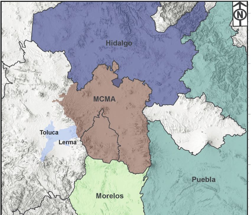
158                                          G. Maldonado Pacheco et al.

      Keywords: CO column, averaging kernel, scaling factor, IASI, WRF-chem.

1. Introduction                                                  Previous studies have been carried out in Mexico
Carbon monoxide (CO) is a gas emitted mainly at              City and its surrounding metropolitan area, such
the surface level by fossil fuels combustion and bio-        as the conducted by de Foy et al. (2007), in which
mass burning (Kerzenmacher et al., 2012, Stremme             vertical column measurements of CO, derived from
et al., 2013). In the atmosphere it is produced and          Fourier Transform Infrared (FTIR) spectrometers,
removed by hydrocarbons oxidation and chemical               were used to constrain the CO emission in models,
reaction with the hydroxyl radical (OH), respectively.       and the CO emission was also evaluated in the inven-
Due to its lifetime of weeks to a few months in the          tory for this region; Stremme et al. (2013) presented
troposphere, depending on where it is analyzed and           a new methodology for estimating CO emissions
the season of the year, CO has been used as an atmo-         on large urban areas based on a top-down approach
spheric transport tracer (Rinsland et al., 2006; de Foy      using FTIR measurements from ground and space
et al., 2007; Funke et al., 2007; Turquety et al., 2008,     (employing the IASI instrument), and Bauduin et al.
2009; George et al., 2009; de Wachter et al., 2012).         (2016) investigated the capability of IASI to retrieve
    CO is not only measured in surface but also at           near-surface CO concentrations and evaluated the
different altitudes employing remote sensing, such           influence of thermal contrast. These works focused
as satellite measurements from the Measurement of            on analyzing CO emissions in Mexico City, but it is
Pollution in the Troposphere (MOPITT), the Scanning          important to study other surrounding regions.
Imaging Absorption Spectrometer for Atmospheric                  Regarding IASI, it is one of the most recent satel-
Chartography (SCIAMACHY), and the Infrared At-               lite instruments that measure CO. It was launched in
mospheric Sounding Interferometer (IASI), among              2006 on board the Metop-A satellite. The field of view
other instruments (Luo et al., 2007; Clerbaux et al.,        is 50 km with four circular measurements of 12 km
2008a; Turquety et al., 2008). These observations can        at nadir and has a swath of 2200 km that allows to
also provide information of CO surface concentrations        observe the planet twice a day (Clerbaux et al., 2009;
and its transport over polluted urban areas (Clerbaux        Hilton et al., 2012). The satellite is sun-synchronous
et al., 2008b; Fortems-Cheiney et al., 2009; Fagbeja         with equator crossing times of 09:30 and 21:30 LT
et al., 2015; Rakitin et al., 2015; Bauduin et al., 2016).   (Clerbaux et al., 2009; Fortems-Cheiney et al., 2009;
    Several studies have been carried out around the         George et al., 2009; Turquety et al., 2009) and the
world employing satellite observations, e.g., Liu            crossing hour over central Mexico is approximately
et al. (2005) studied the MOPPIT detection of CO             at 10:00 LT (Stremme et al., 2013). In addition, IASI
emission from large forest fires in the United States        has a resolution of 0.5 cm–1 in a spectral range from
during 2000; Tanimoto et al. (2009) analyzed CO              645 to 2760 cm–1.
plumes transported from western Siberia toward                   This work aims to reduce the differences between
northern Japan using images from the Atmospheric             the observed and modeled carbon monoxide concen-
Infrared Sounder (AIRS); Kopacz et al. (2009) con-           trations by employing the WRF-Chem model fed with
strained Asian sources of CO by using an atmospheric         the 2008 emissions inventory. To do this, a method-
chemical transport model (GEOS-Chem CTM) and                 ology was applied to compare WRF-Chem and IASI
observations from MOPITT; Klonecki et al. (2012)             data, obtaining scaling factors that allow to update
evaluated the IASI CO product against independent            carbon monoxide emissions for a specific period.
in-situ aircraft and analyzed the impact of eight
months assimilation of IASI CO columns; Marey
et al. (2015) presented a satellite-based analysis to        2. Methodology
explore contributing factors that affect tropospheric        2.1 Model and data description
CO levels over Alberta, Canada, and Rakitin et al.           The WRF-Chem model (Grell et al., 2005; Fast et al.,
(2017) estimated trends of total CO over Eurasia             2006) was used to estimate CO concentrations. The
using information from AIRS.                                 model was fed with NCAR one-degree resolution
CO emissions assessment with model and satellite data 159
meteorological data and two nested domains were semarnat/documentos/documentos-del-inventar-
modeled using the USGS 24-category land-use: the io-nacional-de-emisiones). Its elaboration follows
first one with a 90 by 90 cells mesh grid with 9-km international standards, and it has some quality as-
resolution and the second with an 88 by 88 cells surance procedures for the input, the processing and
mesh grid with 3-km resolution (Fig. 1). February the reporting of information. The annual emissions
2011 was modeled because it was the month with inventory was processed in order to be suitable to use
more available surface measurement data (from a in the WRF-Chem model following the methodology
campaign carried out in the State of Mexico). The presented by García-Reynoso et al. (2018).
parameterizations employed in this work are the Regarding the satellite data, we used the Fast
YSU scheme for the boundary layer (Song-You et Optimal Retrievals on Layers for IASI (FORLI-CO)
al., 2006), the WRF Single-Moment 5-class scheme (https://iasi.aeris-data.fr/CO_IASI_A_data/), which
(WSM5) for microphysics (Song-You et al., 2004), calculates the CO profile in 19 layers with a 1-km
Rapid Radiative Transfer Model scheme (RRTM) thickness in the first 18 layers and up to a 60-km
for the longwave radiation (Mlawer et al., 1997), the altitude in the last one (Hurtmans et al., 2012; de
Goddard scheme for the shortwave radiation (Matsui Wachter et al., 2012). All the CO total column data
et al., 2018) and the Grell-3 scheme for the cumulus were obtained at 10:00 LT, approximately (Stremme
option (Grell, 1993; Grell et al., 2002) et al., 2013), including the averaging kernel matrix,
its associated errors, and the a priori profile, among
N
other values.
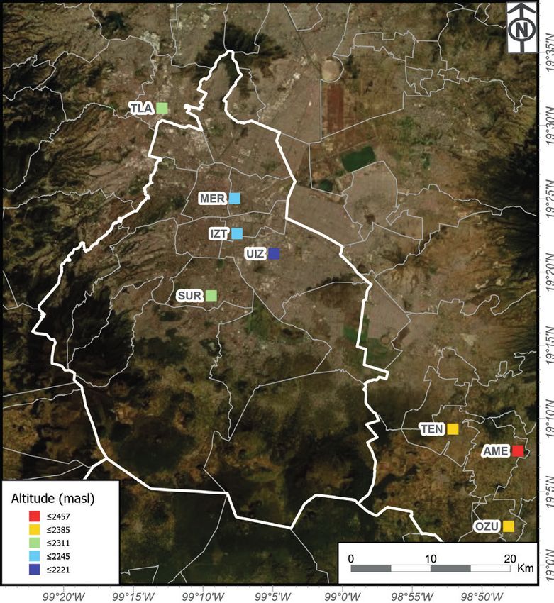
In order to compare the model results against sur-
30°N
face observations, data from five stations of Mexico
City’s Automatic Air Quality Monitoring Network
26°N
(RAMA, Spanish acronym) were used: Iztacalco
(IZT), Merced (MER), Santa Úrsula (SUR), Tlal-
22°N
nepantla (TLA) and UAM Iztapalapa (UIZ). This
monitoring network reports hourly concentrations
of CO, SO2, O2, and NOx, among other chemical
18°N
and meteorological variables. In addition, the United
310 620
States Environmental Protection Agency (USE-
0
km
116°W 112°W 108°W 104°W 100°W 96°W 92°W 88°W
PA) has been performing audits to stations within
Fig. 1. Modeling domains (white squares). The largest Mexico City’s air monitoring network since 2009,
domain has a 9-km resolution and the smallest a 3-km evaluating their systems for station operation and
resolution. calibration (http://www.aire.cdmx.gob.mx/default.
php?opc=%27ZaBhnmI=&dc=%27Zg==).
The 2008 National Emissions Inventory (García- Additionally, data from a surface measurement
Reynoso et al., 2018) was used because at the time of campaign in the State of Mexico were used in the
the analysis only these emission data were available. Amecameca (AME), Tenango (TEN) and Ozumba
The National Emissions Inventory was developed by (OZU) municipalities (Fig. 2).
the Mexican Ministry of Environment and Natural
Resources (SEMARNAT). It includes information 2.2 Modeling procedure
on emissions released into the atmosphere from Dedicated CO emission inventories were created for
criteria pollutants: carbon monoxide (CO), nitrogen the 3-km resolution model domain. These inventories
oxides (NOx), sulfur oxides (SOx) and particles with only have CO emissions for some specific regions:
aerodynamic diameter less than 10 and 2.5 µm (PM10 The Mexico City Metropolitan Area (MCMA), the
and PM2.5), volatile organic compounds (VOCs) and Toluca and Lerma municipalities, and Morelos, Puebla
ammonium (NH 3 ), emitted from area, mobile and Hidalgo states (Fig. 3). A zero-emission value
and fixed sources. It is elaborated periodically and was placed on the remaining domain areas and the
is available from the internet (https://www.gob.mx/ concentration from model boundaries was considered.160 G. Maldonado Pacheco et al.
from model boundaries) with the purpose of knowing
the influence of each region on the others.
19°35'N
2.2.1 Model total column calculation procedure
19°30'N
It is known that the satellite crossing time over central
Mexico is around 10:00 LT (Clerbaux et al., 2009;
19°25'N
Stremme et al., 2013). Therefore, the comparisons
between satellite and modeled data are made at this
time. For this, it is necessary to compute the CO
19°20'N
modeled columns (in molecules per cm2) for each
grid by using the concentration in every level (in parts
19°15'N
per million in volume [ppm]), temperature, pressure
and layer thickness (Lt).
19°10'N
First, the model height of each level and the
thickness of each layer are obtained:
19°5'N
Altitude (masl)
≤2457
≤2385 Z=
( PH + PHB ) (1)
≤2311
≤2245 9.8
19°0'N
≤2221
99°20'W 99°15'W 99°10'W 99°5'W 99°0'W 98°55'W 98°50'W
Lt = Z n+1 Z n (2)
Fig. 2. Location of the measurement stations and their
approximate altitude.
where Lt is the layer thickness (m), Z the level height
in meters (m), PH the geopotential height (m2s–2), and
PHB the geopotential perturbation (m2s–2).
20°30'N
Then, the state equation is used for the calculation
of molecules cm–2:
Molecules number Cco * P * NA* Lt
(3)
20°N
=
cm2 R *T *106
Pmodel + PB
where P = P ( atm) = (4),
19°30'N
101325
Cco is the CO concentration in ppm (mL m–3),
R = 82.57 (mL atm mol–1 K–1), NA is the Avogadro
number (molecules mol–1), Pmodel is the model pres-
19°N
sure (Pa), PB is the pressure perturbation (Pa), and T:
0.284
P
T ( K ) = (Tmodel + 300 ) * (5)
18°30'N
P0
0 20 40
km where Tmodel is the perturbation potential temperature
100°W 99°30'W 99°W 98°30'W 98°W
(θ – T0) (K), (T0 = 300), and P0 the reference pressure
Fig. 3. Metropolitan areas that were used to evaluate the (1 atm).
influence of surrounding cities over the MCMA. Then, this method allows to estimate the modeled
partial columns for each layer in the model.
Subsequently, the WRF-Chem model was run for 2.2.2 Scaling factors calculation procedure
February 1-28, 2011. The chemistry was turned off in or- According to Rodgers and Connor (2003), in order
der to model five tracers (considering the concentration to compare total columns from different instrumentsCO emissions assessment with model and satellite data 161
that have different characteristics and vertical sensi- After that, we calculated the scaling factors using
tivity, it is necessary to perform a data treatment that Eq. (7):
includes some of their characteristics. In this case,
IASI’s averaging kernels were used, which provide y ' = Kx (7)
information about the vertical sensitivity of the re-
trieval to the true state of the atmosphere (Eq. [6a]) where:
(Rodgers, 2000; Luo et al., 2007).
y = y g ( Asat 1) xa (8)
(xsat xa ) = Asat(xtrue xa ) + (6a)
and x is the scaling vector; K the matrix that contains
where xsat is the retrieved profile, xa the IASI a pri- the smoothed total columns for each region and the
ori profile, Asat the IASI’s averaging kernels, xtrue concentration from model boundaries for every co-
the true but unknown profile, and ε the error in the incident point, and y the vector that contains the total
retrieved profile. satellite columns in the coincident points.
For the comparison, we assume that the modeled Solving equation 7 for x:
profile is the true profile.
Therefore, the satellite averaging kernels were x = G • y' (9)
first interpolated to the model heights in each co-
incident point. Next, the modeled CO profiles were where
smoothed by using Eq. (6b):
1
xmodel _ smoothed = A • xmodel + (1 A) • xa (6b)
(
G = KT • K ) • KT (10)
Subsequently, the emissions were scaled by multi-
where xmodel_smoothed is the smoothed model profile, A plying the original emissions from each region by its
the averaging kernel interpolated to model heights, corresponding scaling factor, not only at 10:00 LT but
and xmodel the original model profile. at all times. Afterwards, the model was run using the
In this work we used the satellite total column. scaled emission inventories and chemistry turned on.
Then, the total column operator was applied for Finally, these model results were compared against
modeled partial columns (g = [111111….1]) to sum surface measurements at 10:00 LT, time at which the
up all modeled partial columns: total column analysis was made.
g xmodel _ smoothed = g A • xmodel + ( g g A) • x a (6c)
3. Results
Afterwards, a matrix K was created. Its columns Having performed the procedure described in the
correspond to the smoothed total column values calcu- methodology section, Table I presents the scaling
lated by Eq. (6c) for each region and the concentration
from model boundaries. Its rows indicate the number
of coincident points between the satellite and the
Table I. Scaling factors for February 2011, estimated with
model. Therefore, in this specific work: K (1074,6). respect to the 2008 emissions inventory.
The modeled CO total column of each grid point
and time is a linear combination of different origin Region Scaling factor Uncertainty (%)
CO molecules sum, which is represented by Eq. (6d): Mexico City and
Metropolitan Area 0.43 5.62
xmodel =x 1 xToluca +x 2 x Mexico City +… +x 6 x Boundary (6d) Toluca 0.30 16.28
Morelos 0.44 21.12
g xmodel _ smoothed (g g A) • x a =
(6e)
Puebla
Hidalgo
0.72
2.00
12.98
45.16
gA x 1 xToluca + gAx 2 x Mexico City Boundary 1.86 0.40162 G. Maldonado Pacheco et al.
factors and their associated uncertainties estimated RAMA stations
6000
for each region after comparing modeled and satellite
Concentration (µL/m3)
5000
total columns.
4000
For the MCMA it is observed that the scaling
3000
factor is 0.43, while for Toluca, Morelos and Puebla
2000
it is also less than 1. This means that it is necessary
1000
to reduce the contribution from these regions to the
0
CO total column; therefore, CO emissions must be Original model Scaled model Observations
reduced with respect to the original run. In the case
Fig. 4. Comparison between model and surface observa-
of Hidalgo and the boundary concentration, the scal- tions for RAMA stations (µL/m3).
ing factors are greater than 1, so their contribution
to the total column must increase; consequently, CO
emissions must increase. 1400 State of Mexico
Regarding uncertainties, the smallest are estimat- 1200
Concentration (µL/m3)
ed for the MCMA and the background concentration, 1000
and the greatest are calculated for Morelos and Hi- 800
dalgo. This might be related to lower emissions in 600
these areas. 400
The method considers each region emissions and 200
uses the coincident points to reduce the differences 0
between satellite and modeled data. Because the anal- Original model Scaled model Observations
ysis is done by region and not by coincident point, it Fig. 5. Comparison between model and surface observa-
is possible to estimate a single scaling factor for each tions for stations in the State of Mexico (µL/m3).
region and consequently the differences between the
model data and satellite observations are reduced.
from February 6 to March 8, 2011. In the image, the
3.1 Comparisons between measured data and mo- analysis was carried out in the corresponding period
del results February 6-28, 2011. Again, two modeling cases
After applying the scaling factors, the model was are presented, using original and scaled emissions
run with chemistry turned on. Comparisons between at 10:00 LT.
model results and surface measurements were made It is observed that the model results are higher
in the modeled period at 10:00 LT. The stations are than the measurements when the original emissions
located in Mexico City and its surroundings, and this are used; however, an improvement in the model
analysis can help us to obtain information about the performance is found when the scaled emissions are
model performance at this hour. employed.
Figure 4 shows box plots for the RAMA stations
(Fig. 2) and the model results using original and 3.2 Ratios comparison for modeled and observed
scaled emissions at 10:00 LT, which is approximately data
the satellite crossing hour over central Mexico. In Another method to evaluate inventory emissions out-
general, the model predicts higher concentrations side of Mexico City is to compare observed modeled
than the measurements when original emissions are ratios obtained from surface and total column. This
used; however, when inventories are scaled, model was made for the State of Mexico stations because
results are closer to the observations, indicating an more information, related to meteorological condi-
improvement in the model performance at this time. tions, is available.
Figure 5 shows box plots for the modeled con- García-Yee et al. (2017) observed, from the State
centrations against measurement data obtained from of Mexico campaign, that under low pressure syn-
a campaign made in three locations in the State of optic systems (LPS) southerly winds (from Morelos
Mexico: Amecameca, Ozumba and Tenango (Fig. 2), and Puebla) predominated throughout most of theCO emissions assessment with model and satellite data 163
Table II. Ratio comparison: satellite model versus observations model (surface).
Molecules/cm2 µL/m3 Ratio
Station Satellite Model Surface Model Satellite/ Observations/
observations (surface) model model
AME (HPS) 1.59E+18 1.41E+18 701.45 652.31 1.13 1.08
AME (LPS) 1.34E+18 7.91E+17 430.98 110.32 1.70 3.91
TEN (LPS) 1.30E+18 7.56E+17 80 113.43 1.73 0.71
OZU
(transition) 1.69E+18 1.04E+18 300 206.87 1.63 1.45
AME: Amecameca; TEN: Tenango; OZU: Ozumba; HPS: high pressure synoptic system; LPS: low pressure
synoptic system.
daytime, and under high pressure synoptic systems Tenango and Ozumba is more affected by southerly
(HPS) northerly winds (from Mexico City) dominat- winds (emissions from Morelos and Puebla). On the
ed all morning. contrary, during the warm dry season (from March
In this analysis, the satellite-model (total column) to May), where the HPS are recurrent, the northerly
ratio was compared to the observations-model ratio winds might affect the CO concentration in these
(in surface). Table II shows the modeled and observed sites (emissions from Mexico City) (García-Yee et
(satellite and surface stations) values for the days al., 2017; Molina et al., 2019).
in which satellite information was available for the
area during the campaign period (February 2011). 3.3 Statistics
It would be expected that the ratio of the modeled Table III shows the agreement indexes (Willmott,
and observed concentrations on surface would have 1981) calculated at 10:00 LT for the RAMA stations
the same trend as the ratios obtained from the total and the measurement sites in Amecameca, Tenango
column data because of the prevailing winds. and Ozumba. This statistic is a standardized measure
For Amecameca, both ratios show the same trend of the degree of model prediction error compared to
and are greater than 1, suggesting that the model observations. It can vary from 0, in which case there
predicts correctly the wind direction and underes- is no agreement, to 1, in which case the agreement is
timates the total column and surface concentration. perfect. Besides, Table IV shows the root mean square
For Tenango, under LPS, the satellite-model ratio is error (RMSE) for the same cases as Table III. The
greater than 1, but in surface it is less than 1, so it relative improvement (third column) is calculated
is likely that local effects are relevant to this station
or that the model does not estimate wind direction
properly. And for Ozumba, classified as a transition Table III. Agreement index.
day by García-Yee et al. (2017), the ratios show the
same trends with values greater that 1, indicating Agreement indexes
that the model predicts wind direction correctly and Station Original Scaled Percentage
underestimates the measurements. difference
Note that in this investigation only four points
Iztacalco 0.60 0.62 3.33
were studied, so it would be beneficial to use a greater
Merced 0.54 0.59 9.26
number of comparison points (larger analysis period) Santa Úrsula 0.51 0.59 15.69
and different times of the year because of the LPS Tlalnepantla 0.53 0.60 13.21
and HPS predominance in different seasons. During UAM-Iztapalapa 0.53 0.49 –7.55
the rainy season (from June to October), where Amecameca 0.48 0.56 16.67
LPS systems occurs more frequently, it would be Tenango 0.57 0.74 29.82
expected that the CO concentration in Amecameca, Ozumba 0.54 0.69 27.78164 G. Maldonado Pacheco et al.
with respect to the original so that improvement is corresponds to the model results employing original
positive: (scaled-original)/original for the agree- emissions, the blue line to the model results using the
ment index and (original-scaled)/original for the scaled emissions, and the yellow line to the RAMA
RMSE-measure. measurements. The dotted red line indicates the time
at which the comparison was made (10:00 LT).
Table IV. Root mean square error (µL/m3) It is observed that CO concentrations are reduced
when the scaling factors are applied to the original
Root mean square error (RMSE)
emissions. For Iztacalco, Merced, Santa Úrsula and
Station Original Scaled Percentage Tlalnepantla the scaled CO concentrations are always
difference closer to observations. As for UAM- Iztapalapa, the
Iztacalco 1531.47 1057.58 30.94 original concentrations are closer to observations in
Merced 1571.34 1128.40 28.19 most of the analyzed period, but some days the scaled
Santa Úrsula 1406.09 851.24 39.46 concentrations are closer to the measurements. This
Tlalnepantla 1296.80 854.25 34.13 could be explained by the influence of local factors
UAM-Iztapalapa 1360.07 1548.47 –13.85 related to CO transport from other regions.
Amecameca 315.06 211.83 32.77 In the case of the State of Mexico stations (Fig. 7),
Tenango 417.70 188.13 54.96
Ozumba 212.59 106.75 49.79 different patterns are observed compared to the
RAMA stations. For Amecameca and Ozumba,
the observations are most of the time greater than
As for the agreement index, the model perfor- the model results using either original or scaled
mance is improved (up to 29%) in seven stations: emissions. Regarding Tenango, the original model
Merced, Tlalnepantla, Amecameca, Tenango, Ozum- results are closer to the observations in the hours of
ba, Iztcacalco and Santa Úrsula. For UAM-Iztapa- high concentration from February 13-15, but in other
lapa, a small decrease is observed in its value. The days the difference between scaled concentrations
best agreement is obtained in Tenango using scaled and measurements is smaller. These results suggest
emissions and the worst in Amecameca using orig- that most of the days CO concentrations in these sites
inal emissions. Regarding the RMSE, this statistic do not originate in the MCMA; therefore, the model
decreases for the same seven stations (up to 55%) performance would improve only in days when there
when the scaled emissions are used; so, according is CO coming from the MCMA.
to this statistic, the model performance improve in
these locations at the analysis time. 3.5 Total column comparison
For most stations (except UAM-Iztapalapa) it is Figure 8 shows the differences in molecules cm–2
observed that the results from both statistics agree, between the satellite and the model results using
reducing the average differences between the model the original (a) and scaled (b) inventories, but also
results and the observations (according to RMSE) in percentage employing the original (c) and scaled
and increasing the agreement between the modeled (d) emissions. The greatest difference between the
and observed data (with respect to the agreement satellite and the model is observed when the original
index). As for the UAM-Iztapalapa station, it is pos- inventories are used and decreases when the scaled
sible that the CO concentration is influenced by local inventories are employed; therefore, these results
factors; consequently, it is related to emissions from suggest that the model performance improves after
other regions causing the RMSE to increase and the scaling the carbon monoxide emissions according to
agreement index to decrease slightly when the scaled the total column comparison.
inventories are employed.
3.4 Time series for the RAMA and State of Mexico 4. Conclusions
stations In this paper, a method was presented and applied
The time series for each RAMA station, from Feb- to compare CO total columns from the WRF-Chem
ruary 9-17, are shown in Figure 6. The green line model and the IASI instrument, based on the meth-CO emissions assessment with model and satellite data 165
Concentration (µL/m3)
a) Iztacalco
12000
10000
8000
Observations
6000
Original
4000
Scaled
2000
10 a.m.
0
09-Feb
10-Feb
11-Feb
12-Feb
13Feb
14-Feb
15-Feb
16-Feb
17-Feb
Dates
b) Merced
Concentration (µL/m3)
12000
10000
8000 Observations
6000 Original
4000 Scaled
2000 10 a.m.
0
09-Feb
10-Feb
11-Feb
12-Feb
13Feb
14-Feb
15-Feb
16-Feb
17-Feb
Dates
c)
Santa Úrsula
Concentration (µL/m3)
10000
8000
6000 Observations
Original
4000
Scaled
2000
10 a.m.
0
09-Feb
10-Feb
11-Feb
12-Feb
13Feb
14-Feb
15-Feb
16-Feb
Dates 17-Feb
d) Tlalnepantla
12000
Concentration (µL/m3)
10000
8000
Observations
6000
Original
4000
Scaled
2000
10 a.m.
0
09-Feb
10-Feb
11-Feb
12-Feb
13Feb
14-Feb
15-Feb
16-Feb
17-Feb
Dates
e) UAM Iztapalapa
Concentration (µL/m3)
10000
8000
Observations
6000
Original
4000
Scaled
2000 10 a.m.
0
09-Feb
10-Feb
11-Feb
12-Feb
13Feb
14-Feb
15-Feb
16-Feb
17-Feb
Dates
Fig. 6. Time series for the RAMA stations comparing the original and scaled modeled concentrations
against measurements.166 G. Maldonado Pacheco et al.
a) Amecameca
Concentration (µL/m3)
3000
2500
2000
Observations
1500
Original
1000
Scaled
500
10 a.m.
0
09-Feb
10-Feb
11-Feb
12-Feb
13Feb
14-Feb
15-Feb
16-Feb
17-Feb
Dates
Tenango
Concentration (µL/m3)
1600
1400
1200
1000 Observations
800
Original
600
400 Scaled
200 10 a.m.
0
09-Feb
10-Feb
11-Feb
12-Feb
13Feb
14-Feb
15-Feb
16-Feb
17-Feb
Dates
Ozumba
1800
Concentration (µL/m3)
1600
1400
1200
1000 Observations
800 Original
600
Scaled
400
200 10 a.m.
0
09-Feb
10-Feb
11-Feb
12-Feb
13Feb
14-Feb
15-Feb
16-Feb
17-Feb
Dates
Fig. 7. Time series for the State of Mexico stations comparing the original and scaled modeled con-
centrations against measurements.
odology described by Rodgers and Connor (2003). can exist, the model performance improves in most of
From this comparison, scaling factors were estimated the sites suggesting these types of data can be com-
for different regions using the sensitivity character- pared. The analysis may be done in higher resolution
istics of the instrument (averaging kernels) at the depending on the available computing resources.
satellite crossing time over central Mexico. The It is recommended to perform the analysis over
results are important because if updated emissions a larger period, since this would provide a greater
are not available for a given period, they could be number of comparison points; also, to include other
estimated by this method. satellite instruments such as the Tropospheric Moni-
It is shown that the suggested method works for toring Instrument (TROPOMI) and Measurement of
the IASI instrument at the analysis time reducing the Pollution in the Troposphere (MOPITT), because this
difference between emissions in the 2008 emissions would allow to analyze additional times other than
inventory and the current ones; therefore, the model 10:00 LT as well as the vertical dispersion scheme of
performance improves in the surface level according to the model, which may contribute to the attainment of
the estimated statistics (the agreement index increases different modeled vertical profiles. Since the scaling
up to 29% and the RMSE decreases up to 55%) and the factors must always be interpreted relative to the in-
time series (in which the scaled model concentrations ventory employed, in future works we suggest using
approach to the observations in many cases). other emission inventories as starting points, and
Even though the concentration reported by the then comparing the results. Since the method may
model is a cell of 3 × 3 km, in which several stations be used in other modeled regions and time periodsCO emissions assessment with model and satellite data 167
Differences
a) b)
20.5 20.5
20.0 20.0 1.5
1.0
molec/cm2
Latitude
Latitude
19.5 19.5 0.5
0.0
19.0 19.0 –0.5
–1.0
18.5 18.5 1.5x10¹⁸
–100.0 –99.5 –99.0 –98.5 –98.0 –97.5 –100.0 –99.5 –99.0 –98.5 –98.0 –97.5
Longitude Longitude
Percentages
c) d)
20.5 20.5
100
20.0 20.0
50
Percentage (%)
Latitude
Latitude
19.5 19.5
0
19.0 19.0 –50
–100
18.5 18.5
–100.0 –99.5 –99.0 –98.5 –98.0 –97.5 –100.0 –99.5 –99.0 –98.5 –98.0 –97.5
Longitude Longitude
Fig. 8. Satellite minus (a) original and (b) scaled model (in molecules cm–2). Difference
in column units (molecules cm–2) and percentage using original (a, c) and scaled (b, d)
emissions.
provided there are satellite measurements, it can be this study through a student fellowship, and UNAM
considered as an important tool for investigating DGAPA-PAPIIT IN111418 is also acknowledged for
trends and comparing different megacities. its support in computational infrastructure. We thank
Alejandro Bezanilla Morlot for his support in the use
of the computational infrastructure.
Acknowledgments
IASI is a joint mission of Eumetsat and the Centre
National d’Etudes Spatiales (CNES, France). The References
authors acknowledge the Aeris data infrastructure Bauduin S, Clarisse L, Theunissen M, George M, Hurt-
(http://iasi.aeris-data.fr/CO/) for providing access mans D, Clerbaux C and Coheur P-F. 2016. IASI’s
to the IASI CO data used in this study. The authors sensitivity to near-surface carbon monoxide (CO): The-
also gratefully acknowledge the computing time oretical analyses and retrievals on test cases. Journal of
granted by LANCAD and CONACYT on the su- Quantitative Spectroscopy and Radiative Transfer 189:
percomputer Miztli at DGTIC UNAM and by the 428-440. https://doi.org/10.1016/j.jqsrt.2016.12.022
supercomputing area at the Atmospheric Sciences Clerbaux C, George M, Turquety S, Walker KA, Barret B,
Center (CCA), UNAM. We also thank the support Bernath P, Boone C, Borsdorff T, Cammas JP, Catoire
and work of Bertha Eugenia Mar Morales in the V, Coffey M, Coheur P-F, Deeter M, De Mazière M,
generation of the high-quality images included in this Drummond J, Duchatelet P, Dupuy E, de Zafra R, Ed-
article. CONACYT is acknowledged for founding dounia F, Edwards DP, Emmons L, Funke B, Gille J,168 G. Maldonado Pacheco et al. Griffith DWT, Hannigan J, Hase F, Höpfner M, Jones Evolution of ozone, particulates, and aerosol direct N, Kagawa A, Kasai Y, Kramer I, Le Flochmoën E, radiative forcing in the vicinity of Houston using a Livesey NJ, López-Puertas M, Luo M, Mahieu E, fully coupled meteorology-chemistry-aerosol model. Murtagh D, Nédélec P, Pazmino A, Pumphrey H, Ri- Journal of Geophysical Research 111: D21305. https:// caud P, Rinsland CP, Robert C, Schneider M, Senten doi.org/10.1029/2005JD006721 C, Stiller G, Strandberg A, Strong K, Sussmann R, Fortems-Cheiney A, Chevallier F, Pison I, Bousquet P, Thouret V, Urban J and Wiacek A. 2008a. CO mea- Carouge C, Clerbaux C, Coheur P-F, George M, Hurt- surements from the ACE-FTS satellite instrument: data mans D and Szopa S. 2009. On the capability of IASI analysis and validation using ground-based, airborne measurements to inform about CO surface emissions. and spaceborne observations. Atmospheric Chemistry Atmospheric Chemistry and Physics 9: 8735-8743. and Physics 8: 2569-2594. https://doi.org/10.5194/ https://doi.org/10.5194/acp-9-8735-2009 acp-8-2569-2008 Funke B, López-Puertas M, Bermejo-Pantaleón D, von Clerbaux C, Edwards DP, Deeter M, Emmons L, La- Clarmann T, Stiller GP, Höpfner M, Grabowski U and marque J-F, Tie X X, Massie ST and Gille J. 2008b. Kaufmann M. 2007. Analysis of nonlocal thermody- Carbon monoxide pollution from cities and urban namic equilibrium CO 4.7 mm fundamental, isotopic, areas observed by the Terra/MOPITT mission. Geo- and hot band emissions measured by the Michelson physical Research Letters 35: L03817. https://doi. Interferometer for Passive Atmospheric Sounding org/10.1029/2007GL032300 on Envisat. Journal of Geophysical Research 112: Clerbaux C, Boynard A, Clarisse L, George M, Had- D11305. https://doi.org/10.1029/2006JD007933 ji-Lazaro J, Herbin H, Hurtmans D, Pommier M, Ra- García-Reynoso JA, Mar-Morales BE and Ruiz-Suárez zavi A, Turquety S, Wespes C and Coheur P-F. 2009. LG. 2018. Modelo de distribución espacial, tempo- Monitoring of atmospheric composition using the ral y de especiación del inventario de emisiones de thermal infrared IASI/MetOp sounder. Atmospheric México (año base 2008) para su uso en modelización Chemistry and Physics 9: 6041-6054. https://doi. de calidad del aire (DiETE). Revista Internacional de org/10.5194/acp-9-6041-2009 Contaminación Ambiental 34 (4): 635-649. https://doi. De Foy B, Lei W, Zavala M, Volkamer R, Samuelsson J, org/10.20937/RICA.2018.34.04.07 Mellqvist J, Galle B, Martínez A-P, Grutter M, Retama García-Yee JS, Torres-Jardón R, Barrera-Huertas H, Castro A and Molina LT. 2007. Modelling constraints on the T, Peralta O, García M, Gutiérrez W, Robles M, Tor- emission inventory and on vertical dispersion for CO res-Jaramillo JA, Ortínez Álvarez A and Ruiz-Suárez and SO2 in the Mexico City Metropolitan Area using LG. 2017. Characterization of NOx-Ox relationships Solar FTIR and zenith sky UV spectroscopy. Atmo- during daytime interchange of air masses over a moun- spheric Chemistry and Physics 7: 781-801. https://doi. tain pass in the Mexico City megalopolis. Atmospheric org/10.5194/acp-7-781-2007 Environment 177: 100-110. https://doi.org/10.1016/j. De Wachter E, Barret B, Le Flochmoën E, Pavelin E, atmosenv.2017.11.017 Matricardi M, Clerbaux C, Hadji-Lazaro J, George George M, Clerbaux C, Hurtmans D, Turquety S, Co- M, Hurtmans D, Coheur P-F, Nedelec P and Cammas heur P-F, Pommier M, Hadji-Lazaro J, Edwards JP. 2012. Retrieval of MetOp-A/IASI CO profiles DP, Worden H, Luo M, Rinsland C and McMillan and validation with MOZAIC data. Atmospheric W. 2009. Carbon monoxide distributions from the Measurements Techniques 5: 2843-2857. https://doi. IASI/METOP mission: Evaluation with other space- org/10.5194/amt-5-2843-2012 borne remote sensors. Atmospheric Chemistry and Fagbeja MA, Hill JL, Chatterton TJ and Longhurst JWS. Physics 9: 8317-8330. https://doi.org/10.5194/acp- 2015. A GIS-based assessment of the suitability of 9-8317-2009 SCIAMACHY satellite sensor measurements for es- Grell GA. 1993. Prognostic evaluation of assumptions timating reliable CO concentrations in a low-latitude used by cumulus parameterizations. Monthly Weather climate. Environmental Monitoring and Assessment Review 121: 764-787. https://doi.org/10.1175/1520-0 187: 4227. https://doi.org/10.1007/s10661-014-4227-2 493(1993)1212.0.CO;2 Fast JD, Gustafson WI Jr, Easter RC, Zaveri RA, Barnard Grell GA and Dévényi D. 2002. A generalized approach JC, Chapman EG, Grell GA and Peckham SE. 2006. to parameterizing convection combining ensemble and
CO emissions assessment with model and satellite data                               169

   data assimilation techniques. Geophysical Research            lytical Bayesian inversion methods for constraining
   Letters 29 (14). https://doi.org/10.1029/2002GL015311         Asian sources of carbon monoxide using satellite
Grell GA, Peckham SE, Schmitz R, McKeen SA, Frost G,             (MOPITT) measurements of CO columns. Journal
   Skamarock WC and Eder B. 2005. Fully coupled “on-             of Geophysical Research 114: D04305. https://doi.
   line” chemistry within the WRF model. Atmospheric             org/10.1029/2007JD009264
   Environment 39: 6957-6975. https://doi.org/10.1016/j.      Liu J, Drummond JR, Li Q, Gille JC and Ziskin DC. 2005.
   atmosenv.2005.04.027                                          Satellite mapping of CO emission from forest fires in
Hilton F, Armante R, August T, Barnet C, Bouchard                Northwest America using MOPITT measurements.
   A, Camy-Peyret C, Capelle V, Clarisse L, Clerbaux             Remote Sensing of Environment 95: 502-516. https://
   C, Coheur P-F, Collard A, Crevoisier C, Dufour G,             doi.org/10.1016/j.rse.2005.01.009
   Edwards D, Faijan F, Fourrié N, Gambacorta A,              Luo M, Rinsland CP, Rodgers CD, Logan JA, Worden
   Goldberg M, Guidard V, Hurtmans D, Illingworth                H, Kulawik S, Eldering A, Goldman A, Shepard M
   S, Jacquinet-Husson N, Kerzenmacher T, Klaes D,               W, Gunson M and Lampel M. 2007. Comparison of
   Lavanant L, Masiello G, Matricardi M, McNally T,              carbon monoxide measurements by TES and MOPITT:
   Newman S, Pavelin E, Payan S, Péquignot E, Peyri-             Influence of a priori data and instrument characteris-
   dieu S, Phulpin T, Remedios J, Schlüssel P, Serio C,          tics on nadir atmospheric species retrievals. Journal
   Strow L, Stubenrauch C, Taylor J, Tobin D, Wolf W             of Geophysical Research 112: D09303. https://doi.
   and Zhou, D. 2012. Hyperspectral earth observation            org/10.1029/2006JD007663
   from IASI: Five years of accomplishments. Bulletin         Marey HS, Hashisho Z, Fu L and Gille J. 2015. Spatial
   of the American Meteorological Society 93: 347-370.           and temporal variation in CO over Alberta using mea-
   https://doi.org/10.1175/BAMS-D-11-00027.1                     surements from satellites, aircraft, and ground stations.
Hurtmans D, Coheur P-F, Wespes C, Clarisse L, Scharf             Atmospheric Chemistry and Physics 15: 3893-3908.
   O, Clerbaux C, Hadji-Lazaro J, George M and Tur-              https://doi.org/10.5194/acp-15-3893-2015
   quety S. 2012. FORLI radiative transfer and retrieval      Matsui T, Zhang SQ, Tao W-K, Lang S, Ichoku C and
   code for IASI. Journal of Quantitative Spectroscopy           Peters-Lidard C. 2018. Impact of radiation frequency,
   and Radiative Transfer 113: 1391-1408. https://doi.           precipitation radiative forcing, and radiation column
   org/10.1016/j.jqsrt.2012.02.036                               aggregation on convection-permitting West African
Kerzenmacher T, Dils B, Kumps N, Blumenstock T, Cler-            monsoon simulations. Climate Dynamics 55: 193-213.
   baux CC, Coheur P-F, Demoulin P, García O, George             https://doi.org/10.1007/s00382-018-4187-2
   M, Griffith DWT, Hase F, Hadji-Lazaro J, Hurtmans          Mlawer EJ, Taubman SJ, Brown PD, Iacono MJ and
   D, Jones N, Mahieu E, Notholt J, Paton-Walsh C,               Clough SA. 1997. Radiative transfer for inhomoge-
   Raffalski U, Ridder T, Schneider M, Servais C and de          neous atmospheres: RRTM, a validated correlated-k
   Mazière M. 2012. Validation of IASI FORLI carbon              model for the longwave. Journal of Geophysical
   monoxide retrievals using FTIR data from NDACC.               Research 102: 16663-16682. https://doi.org/10.1029/
   Atmospheric Measurements Techniques 5: 2751-2761.             97JD00237
   https://doi.org/10.5194/amt-5-2751-2012                    Molina LT, Velasco E, Retama A and Zavala M. 2019.
Klonecki A, Pommier M, Clerbaux C, Ancellet G, Cammas            Experience from Integrated Air Quality Management
   J-P, Coheur P-F, Cozic A, Diskin GS, Hadji-Lazaro             in the Mexico City Metropolitan Area and Singa-
   J, Hauglustaine DA, Hurtmans D, Khattatov B, La-              pore. Atmosphere 10: 512. https://doi.org/10.3390/
   marque J-F, Law KS, Nedelec P, Paris J-D, Podolske            atmos10090512
   JR, Prunet P, Schlager H, Szopa S and Turquety S.          Rakitin VS, Shtabkin YA, Elansky NF, Pankratova NV,
   2012. Assimilation of IASI satellite CO fields into a         Skorokhod AI, Grechko EI and Safronov AN. 2015.
   global chemistry transport model for validation against       Comparison results of satellite and ground-based
   aircraft measurements. Atmospheric Chemistry and              spectroscopic measurements of CO, CH4, and CO2
   Physics 12: 4493-4512. https://doi.org/10.5194/acp-           total contents. Atmospheric and Oceanic Optics 28:
   12-4493-2012                                                  533-542. https://doi.org/10.1134/S1024856015060135
Kopacz M, Jacob DJ, Henze DK, Heald CL, Streets DG            Rakitin VS, Elansky NF, Pankratova NV, Skorokhod
   and Zhang Q. 2009. Comparison of adjoint and ana-             AI, Dzhola AV, Shtabkin YA, Wang P, Wang G,
170                                          G. Maldonado Pacheco et al.

   Vasilieva AV, Makarova MV and Grechko EI. 2017.           Stremme W, Grutter M, Rivera C, Bezanilla A, García AR,
   Study of trends of total CO and CH4 contents over             Ortega I, George M, Clerbaux C, Coheur P-F, Hurtmans
   Eurasia through analysis of ground-based and satel-           D, Hannigan JW and Coffey MT. 2013. Top-down esti-
   lite spectroscopic measurements. Atmospheric and              mation of carbon monoxide emissions from the Mexico
   Oceanic Optics 30: 517-526. https://doi.org/10.1134/          Megacity based on FTIR measurements from ground
   S1024856017060112                                             and space. Atmospheric Chemistry and Physics 13:
Rinsland CP, Luo M, Logan JA, Beer R, Worden H, Ku-              1357-1376. https://doi.org/10.5194/acp-13-1357-2013.
   lawik SS, Rider D, Osterman G, Gunson M, Eldering         Tanimoto H, Sato K, Butler T, Lawrence MG, Fisher JA,
   A, Goldman A, Shepard M, Shepard AC, Clough                   Kopacz M, Yantosca RM, Kanaya Y, Kato S, Okuda
   SA, Rodgers C, Lampel M and Chiou L. 2006. Nadir              T, Tanaka S and Zeng J. 2009. Exploring CO pollution
   measurements of carbon monoxide distributions by              episodes observed at Rishiri Island by chemical weath-
   the Tropospheric Emission Spectrometer instrument             er simulations and AIRS satellite measurements: long-
   onboard the Aura Spacecraft: Overview of analy-               range transport of burning plumes and implications
   sis approach and examples of initial results. Geo-            for emissions inventories. Tellus Series B-Chemical
   physical Research Letters 33: L22806. https://doi.            and Physical Meteorology 61: 394-407. https://doi.
   org/10.1029/2006GL027000                                      org/10.1111/j.1600-0889.2008.00407.x
Rodgers CD. 2000. Inverse methods for atmospheric            Turquety S, Clerbaux C, Law K, Coheur P-F, Cozic A, Szopa
   sounding. Theory and practice. Series on Atmospheric,         S, Hauglustaine DA, Hadji-Lazaro J, Gloudemans AMS,
   Oceanic and Planetary Physics, vol. 2. World Scientific       Schrijver H, Boone CD, Bernath PF and Edwards DP.
   Publishing. https://doi.org/10.1142/3171                      2008. CO emission and export from Asia: An analysis
Rodgers CD and Connor BJ. 2003. Intercomparison of               combining complementary satellite measurements
   remote sounding instruments. Journal of Geophys-              (MOPITT, SCIAMACHY and ACE-FTS) with global
   ical Research 108: 4116. https://doi.org/10.1029/             modeling. Atmospheric Chemistry and Phyisics 8: 5187-
   2002JD002299                                                  5204. https://doi.org/10.5194/acp-8-5187-2008
Song-You H, Dudhia J and Chen S-H. 2004. A re-               Turquety S, Hurtmans D, Hadji-Lazaro J, Coheur P-F,
   vised approach to ice microphysical processes                 Clerbaux C, Josset D and Tsamalis C. 2009. Tracking
   for the bulk parameterization of clouds and pre-              the emission and transport of pollution from wild-
   cipitation. Monthly Weather Review 132: 103-                  fires using the IASI CO retrievals: Analysis of the
   120. https://doi.org/10.1175/1520-0493(2004)132<              summer 2007 Greek fires. Atmospheric Chemistry
   0103:ARATIM>2.0.CO;2                                          and Phyisics 9: 4897-4913. https://doi.org/10.5194/
Song-You H, Noh Y and Dudhia J. 2006. A new vertical             acp-9-4897-2009
   diffusion package with an explicit treatment of en-       Willmott CJ. 1981. On the validation of models. Physical
   trainment processes. Monthly Weather Review 134:              Geography 2: 184-194. https://doi.org/10.1080/02723
   2318-2341. https://doi.org/10.1175/MWR3199.1                  646.1981.10642213
You can also read