Study Guide Land Surface Process Modelling (GEO4 - 4406) - Release 2020 - 2021 Derek Karssenberg
←
→
Page content transcription
If your browser does not render page correctly, please read the page content below
Study Guide Land Surface Process
          Modelling (GEO4 - 4406)
                    Release 2020 - 2021

                    Derek Karssenberg

                              Feb 05, 2021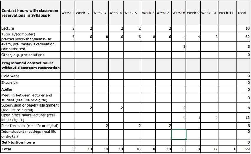
CONTENTS

       i
ii
Study Guide Land Surface Process Modelling (GEO4 - 4406), Release 2020 - 2021

Download this website as pdf.
This document is online at http://karssenberg.geo.uu.nl/lspm

CONTENTS                                                                                        1
Study Guide Land Surface Process Modelling (GEO4 - 4406), Release 2020 - 2021

2                                                                               CONTENTS
CHAPTER

                                                      ONE

                                                 CONTENTS

1.1 Course information

1.1.1 General information

Name of course: Land Surface Process Modelling
Course Code: GEO4-4406
ECTS: 7.5
Category / Level: M (Master)
Teaching period: 3
Contact hours: appr. 6 h / week
Language of instruction: English

1.1.2 Lecturers

Prof. Dr. Derek Karssenberg (coordinator)
Department of Physical Geography
Faculty of Geosciences
Utrecht University
http://karssenberg.geo.uu.nl
-
Kor de Jong
Dr. Oliver Schmitz
Safaa Naffaa
Lars Groeneveld
Department of Physical Geography
Faculty of Geosciences
Utrecht University

                                                          3
Study Guide Land Surface Process Modelling (GEO4 - 4406), Release 2020 - 2021
1.1.3 Place in curriculum and entry requirements
The course provides a theoretical and practical basis of spatio-temporal (process-based) modelling of land surface
processes, and is relevant for all disciplines related to land surface processes (hydrology, land degradation, geomor-
phology, natural hazards, ecology). In addition is provides a background in geoinformatics which is relevant for
appropriate use of modelling tools and GIS.
Entry requirements: you must have study entrance permit.
1.1.4 Aims and content
Domain related
Numerical simulation models of processes on the earth surface are essential tools in fundamental and applied research
in the geosciences. They are used in almost all disciplines in the geosciences, for instance hydrology, geomorphology,
land degradation, sedimentology, and most fields in ecology. They are important instruments in research for a number
of reasons. First, they provide understanding of how systems work, in particular how system components interact,
how systems react to changes in drivers, and how non-linear responses emerge. Also, simulation models can be used
to forecast systems, which is essential in planning and decision making. Finally, land surface process models provide
a means to evaluate theory of simulated processes against observational data.
In this course we will focus on generic principles of land surface modelling. You will study a number of different
approaches to represent land surface processes in a simulation model, including differential equations, rule based
modelling, cellular automata, individual (agent) based approaches, and probabilistic models. We will discuss how
local interactions in large systems can lead to complexity and the impliction of this for forecasting. Also, you will
learn how to combine information from observational data and simulation models using error propagation, calibration,
and data assimilation techniques.
During the course you will learn how these principles can be applied in a number of different disciplines, in particular in
the field of hydrology, geomorphology, sedimentology, and ecology. You will also learn how very similar approaches
are used in other fields, for instance in urban geography and social sciences.
In addition to principles of land surface modelling, you will learn how to use software tools for land surface modelling.
You will study theoretical concepts of software environments for land surface modelling, and you will learn how to
program land surface models. In this part of the course we will use the Python programming language and PCRaster.
These tools provide standard frameworks for model construction and techniques to combine a model with observa-
tional data. Other tools for model construction use similar concepts, so you will be able to apply your knowledge from
this course to other software environments.
The course aims are:
• To retrieve a theoretical basis of land surface modelling, including approaches to represent processes and ap-
proaches to combine data and models.
• To retrieve an understanding of how various systems in the geosciences are represented with land surface models.
• To learn principles of software environments for modelling and how to use these software environments.
4 Chapter 1. ContentsStudy Guide Land Surface Process Modelling (GEO4 - 4406), Release 2020 - 2021
Transferable skills related
• Ability to work in a team: Oral presentations and the case study report are written in teams of 2-3 students.
Students will learn how to distribute the work over team members and how to cooperate efficiently.
• Written communication skills: Three two-page papers are written on which students get extensive feedback
from the tutor. In addition, a longer case study report is written structured like a scientific article.
• Problem-solving skills: Students learn to execute all phases of numerical model construction. This requires
to solve problems related to concepts of process-based models, the implementation of these models using a
programming environment, and the use of various empirical data linked to models. Students are challenged
considerably regarding this aspect in the case study project at the end of the course which is done largely
without support from the tutor.
• Verbal communication skills: Students present their work in two working group sessions. This teaches them
mainly to prepare a well-structured talk in the time span of a few days; in addition they get limited feedback on
the quality of the presentation.
• Strong work ethic: The course is taught as a blended learning course which means that students need to properly
plan their own work.
• Initiative: Students are trained to take initiative, particularly in the case study projects.
• Analytical/quantitative skills: A large part of the course relates to various analytical approaches used in forward
process-based modelling. Students have to apply these approaches in their own modelling work.
• Technical skills: The course teaches computational thinking in particular during the computer labs on Python
programming and PCRaster programming.
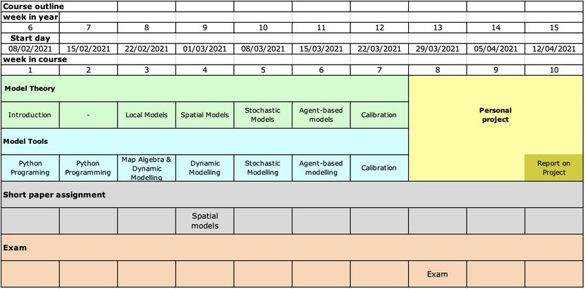
1.1.5 Course outline (time table)
Course outline and schedule are provided in this document. You can also use https://mytimetable.uu.nl to get access
to the schedule (like with all Utrecht University courses).
As shown in the outline of the course in the table below, the course consists of two blocks, Model Theory and Model
Tools. These are run parallel in time. Model theory contains eLectures, a working group meeting, and a paper
assignment. Model Tools is taught mainly using computer practicals. At the end of the course you will do a personal
project, consisting of a case study model and a written report. The detailed course schedule below gives the date and
location of lectures, working groups, and computer practicals. It also provides due dates for the computer practicals
and other assignments.
Important: this course is taught following the flipped teaching model, which implies that theory is learned mainly
through self study while contact hours are used for discussion and questions. Note that a large part of the theory is
provided as pre-recorded eLectures instead of real-time lectures. It is strongly recommended to follow the general
course outline below strictly, also during self study (e.g. watch eLectures and read the text in the reader related to a
topic in the week the topic is scheduled in the general course outline below). Of course you can allow yourself some
flexibility regarding the e-lectures, it is not forbidden to work ahead of time, of course.
1.1. Course information 5Study Guide Land Surface Process Modelling (GEO4 - 4406), Release 2020 - 2021
1.1.6 Calculation of final mark
For passing the course students need to:
• Submit answers to the questions of all computer labs (before the deadline).
• Active participation in working groups.
• Hand-in short paper assignment and report on the personal project in time.
• Get a final mark of 5.5 or higher.
The final mark M is calculated as:
M = 0.1A + 0.65B + 0.25C
with A, the mark for the short paper assignment, B, the mark for the exam, and C, the mark for the written report on
the personal project. A, B, and C are not rounded.
Absence (for instance as a result of illness or family circumstances) during the exam must be agreed with the coordi-
nator of the course in advance by phone or email. You need to hand over a sick note (medical certificate from your
doctor) afterwards to get access to a resit.
The course has been passed if the final grade is >=5.5 and all obligations have been fulfilled. If not, and only if 1) the
final grade is 4.00 or higher and 2) all obligations have been fulfilled, a supplementary test (or repeat exam) can be
offered. If the supplementary test has been successfully passed, the final grade of the course will be 6.0.
For details on the above and further information, see the OER (Education and Examination Regulations).
6 Chapter 1. ContentsStudy Guide Land Surface Process Modelling (GEO4 - 4406), Release 2020 - 2021
1.1.7 Study material
For the exam, you need to study:
• All material indicated in this document as ‘Literature for exam’. You can download this as one PDF (or order it
as a printed syllabus, recommended) from Blackboard.
• Think Python, An introduction to software design, 2nd Edition (!), A. Downey, 2015, Green Tea Press, Need-
ham, 222 pp. Chapters 1, 2, 3, 5, 6, 7, 8, 10, and 14. Online at http://greenteapress.com/wp/think-python-2e/ or
order a print from Blackboard.
• All computer practicals to the extend that you need to understand the core concepts of the tools.
• All eLectures.
Note that material indicated in this document as ‘Reading material’ is background material only. It is recommended
to read through this but it is not a requirement for the exam.
1.1.8 Exam
The written exam will take place at a distance, i.e. at home. Important information related to the exam:
• The exam will be open book. You are allowed to use any source of information or software tool except infor-
mation that you get from other persons.
• Study the study material as described in the studyguide.
• One or two days before the exam you will receive a research paper by e-mail. The paper will be on the design
or use of a simulation model. Read through the paper 2 or 3 times to be sure you understand it. See below on
how the paper is used in the exam.
• The exam will contain a few questions that you need to answer in the context of the paper that you received (see
above). For instance: Is the model used in the paper your read a physically-based model or a conceptual model?
(note that I will not ask this particular question). So the questions will be general, but in the context of the paper.
In addition the exam will contain normal (and open, not multiple choice questions, for instance) on the study
materials.
• Just before the exam starts you will receive (at your students.uu.nl e-mail) the exam questions and a Microsoft
Word file that you can use to type in your answers (it will only contain the numbers of the questions and maybe
some other info). You are of course free to use another text processing software to write down your answers.
• Before the end of the exam you upload your answers to Blackboard. You can do this at an Assignment link with
his purpose (similar link like used for the short paper assignment). In case the upload does not work for some
reason, please e-mail the exam to d.karssenberg@uu.nl).
• Contact Derek Karssenberg in Teams in case you have questions during the exam. E.g. if a question is unclear.
If Teams does not work, send an e-mail (d.karssenberg@uu.nl).
• Try to find a quiet place to take the exam.
1.1. Course information 7Study Guide Land Surface Process Modelling (GEO4 - 4406), Release 2020 - 2021
1.1.9 OSIRIS information on the course
Additional information is available at https://www.osiris.universiteitutrecht.nl/osistu_ospr/StartPagina.do
1.1.10 Online teaching
Our course will almost completely run online. However there will be considerable time for online communication and
extensive feedback will be provided.
The course is run largely following the flipped-teaching model. The idea of flipped teaching is that contact time
between student and tutor is not used for explaining theory but mainly for discussion and questions related to the
theory. To make this work, it is important students study the learning materials before attending an online and realtime
Question Based eLecture. The time schedule of our course supports this approach to learning. Each week, students will
study one particular topic. The first days of the week, or if possible even the week before, it is strongly recommended
to study the learning materials related to this topic. This includes pre-recorded eLectures as well as literature. On
Wednesday, then, we have a so-called Question Based Lecture during which students can ask questions or particular
concepts can be discussed. Students are asked to prepare for this Question Based Lecture by compiling a list of
questions they have. You can ask questions by copy-pasting them in the Chat during the Question Based Lecture or by
just raising you hand during the lecture.
The components of the course are:
• Recorded eLectures, you can listen to these anytime
• Literature, sections from books or scientific articles
• Question Based eLectures, weekly online meeting for questions on study materials, theory or anything important
to the course
• Computer Labs, scheduled computer labs with online supervision
• eLecture, introductionary eLecture at the start of the course
• Working group session
• Short paper assignment
Communication is through:
• MS Teams, ask general questions in the General channel and during contact hours, in particular lab hours, tutors
are online to support you
• E-mail, for other questions, e-mail the course coordinator
• Blackboard, used for uploading your answers to questions in the labs and other assignments
The exam will most likely be on Campus but this is not certain at the time of writing.
1.1.11 Disclaimer due to COVID-19
Due to Covid-19 restrictions, it may be necessary to make last minute changes to the course compared to what has been
described in this manual. E.g. lectures or exams may be held online or an exam may be replaced by an assignment.
The course coordinator will keep students up to date with the latest information.
8 Chapter 1. ContentsStudy Guide Land Surface Process Modelling (GEO4 - 4406), Release 2020 - 2021
1.2 Model Theory
1.2.1 Introduction to land surface process modelling, week 1-2
Key topics
• General introduction to land surface process modelling.
• Forward modelling
• Aims of modelling
• Model development cycle
Literature for exam
Wainwright, J. and Mulligan, M., 2004, Modelling and model building, in: Environmental Modelling: finding sim-
plicity in complexity, Second Edition. J. Wainwright, M. Mulligan (eds), p. 7-26, Wiley, Chichester.
Karssenberg, D., 2010, Introduction to dynamic spatial environmental modelling.
Burrough, P.A., McDonnel, R. & Lloyd, C.D., 2015, Principles of Geographical Information Systems, Oxford Univer-
sity press, Chapter 12, Space-time modelling and error propagation, p. 251-260.
Reading material
Karssenberg, D., Bridge, J.S., 2008, A three-dimensional numerical model of sediment transport, erosion and deposi-
tion within a network of channel belts, flodplain and hill slope: extrinsic and intrinsic controls on floodplain dynamics
and alluvial architecture, Sedimentology, 55, 1717-1745. Link.
Lectures, e-Lectures
Lecture slides Introduction to the course
e-Lecture Introduction to simulation modelling
Lecture slides Introduction to simulation modelling
1.2.2 Local models, week 3
Key topics
• Dynamic point models
• Numerical solution of differential equations
1.2. Model Theory 9Study Guide Land Surface Process Modelling (GEO4 - 4406), Release 2020 - 2021
Literature for exam
Kreyszig, E., 1999, Numerical Methods for Differential Equations, in Advanced Engineering Mathematics, New York,
N.Y., Wiley: p. 942-952.
Lectures, e-Lectures
e-Lecture Point models and differential equations - 01
e-Lecture Point models and differential equations - 02
e-Lecture Point models and differential equations - 03
Lecture slides Point models and differential equations - 01
Lecture slides Point models and differential equations - 02
Lecture slides Point models and differential equations - 03
Answers to three exercises from powerpoint
1.2.3 Spatial models, week 4
Key topics
• Neighbourhood interaction
• Neighbourhoods by a defined topology
• Dynamic neighbourhood models: cellular automata
Literature for exam
Burrough, P.A., McDonnel, R. & Lloyd, C.D., 2015, Principles of Geographical Information Systems, Oxford Univer-
sity press, Chapter 7, Analysis of discrete entities in space, p. 127-145, and Chapter 10, Analysis of continuous fields,
p. 201-229.
Favis-Mortlock, D., 2004, Non-linear dynamics, self-organization and cellular automata models, in: Environmental
Modelling: finding simplicity in complexity, J. Wainwright, M. Mulligan (eds), p. 45-67, Wiley, Chichester.
Reading material
Saco, P.M., Willgoose, G.R., Hancock, G.R., 2007, Eco-geomorphology of banded vegetation patterns in arid and
semi-arid regions, Hydrology and Earth System Sciences, 11: 1717-1730. Link.
10 Chapter 1. ContentsStudy Guide Land Surface Process Modelling (GEO4 - 4406), Release 2020 - 2021
Lectures, e-Lectures
e-Lecture Neighbourhood interaction
e-Lecture slides Spatio-temporal models: neighbourhood interaction, pdf
Working group session
We will have a working group session on this topic.
To prepare for the session:
• Listen to the e-Lecture (see above for the link)
• Study the literature for the exam (related to this topic, see above)
• Create a group (consisting of two students) in Blackboard, available at Course Content -> Working Groups
• Prepare a 10 minute presentation (one per group), for topics see below
During the working group session:
• Presentations are given in MS Teams
• Each group gives a 10 minute presentation
• After each presentation: 5 minutes discussion with questions
The presentation should describe an example of either 1) the use of cellular automata or 2) self organisation in the earth
sciences (or related fields). Search the literature (use a bibliographic database, e.g. http://www.scopus.com) to find
at least one paper on one these topics (examples of applications of cellular automata are land use change, forest fire,
vegetation growth and dispersal, disease spreading, lava flows; for self organisation there are also many examples).
Prepare a presentation which explains how cellular automata are used in the article or what kind of self organisation is
described. If you want you can add items for discussion at the end.
Short paper assignment
Favis-Mortlock (2004, in the reader) discusses self-organizing systems and why feedback mechanisms may lead to
self-organization. Read the paper by Saco et al. (reading material). In a short paper (max. 1000 words excluding
the bibliography, not longer), explain the concept of self-organization and discuss why the system studied by Saco
et al. is a self-organizing system. In addition, provide the main feedback mechanisms that lead to the observed
self-organization. Hand in by uploading in Blackboard.
1.2.4 Stochastic models, week 5
Key topics
• Stochastic variables
• Probability distributions, categorial and continuous variables
• Properties of probability distributions: percentiles, confidence intervals
• Stochastic variables to represent uncertain model inputs and parameters
• Solving stochastic models: Monte Carlo simulation
1.2. Model Theory 11Study Guide Land Surface Process Modelling (GEO4 - 4406), Release 2020 - 2021
Literature for exam
Karssenberg, D. de Jong, K., 2005, Dynamic environmental modelling in GIS: 2. Modelling error propagation. Inter-
national Journal of Geographical Information Science, 19, p. 623-637.
Karssenberg, D., Schmitz, O., Salamon, P., De Jong, K. and Bierkens, M.F.P., 2010, A software framework for con-
struction of process-based stochastic spatio-temporal models and data assimilation. Environmental Modelling & Soft-
ware, 25, pp. 489-493.
Kreyszig, E., 1999, Data Analysis. Probability Theory, in Advanced Engineering Mathematics, New York, N.Y.,
Wiley, Chapter 22, the following pages:
• Pages 1050-1064, except 22.4 (Permutations and Combinations), Problem Sets and Examples
Reading material
No reading material.
e-Lectures
e-Lecture Introduction to Stochastic Modelling
e-Lecture Monte Carlo simulation
e-Lecture slides Stochastic models, Monte Carlo simulation, pdf
Lecture, Q&A session
During a Q&A session (it appears as ‘lecture’ in the course schedule) your tutor will answer questions related to this
topic. You can also ask questions related to other topics that were treated during the course.
To prepare for the session:
• Listen to the e-Lectures on Stochastic Modelling and Monte Carlo simulation (see above for the links)
• Study the literature for the exam (related to this topic, see above)
• E-mail Derek Karssenberg (d.karssenberg@uu.nl) questions at least 1 day in advance of the Q&A session, we
will discuss these topics during the Q&A.
1.2.5 Agent-based models, week 6
Key topics
• Agents vs Fields
• Agent representations
• Examples
12 Chapter 1. ContentsStudy Guide Land Surface Process Modelling (GEO4 - 4406), Release 2020 - 2021
Literature for exam
Macal, C.M., North, M.J., 2010, Tutorial on agent-based modelling and simulation. Journal of Simulation, 4, pp.
151-162.
Reading material
Bennett, D.A., Tang, W., 2006, Modelling adaptive, spatially aware, and mobile agents: Elk migration in Yellowstone.
International Journal of Geographical Information Science, 20, pp. 1039-1066. Link.
Railsback, S.F., 2001, Concepts from complex adaptive systems as a framework for individual-based modelling. Eco-
logical modelling, 139, pp. 47-62. Link.
e-Lectures
e-Lecture Spatial agent-based modelling
Lecture slides Introduction to spatial agent-based modelling, pdf
1.2.6 Calibration, week 7
Key topics
• Objective function
• Minimizing the objective function: hillclimbing, brute force and other techniques
Literature for exam
Beven, K.J., 2002, Parameter estimation and predictive uncertainty, in Rainfall-runoff modelling, the primer, Wiley,
Chichester, p. 217-233.
Janssen, P.H.M, Heuberger, P.S.C., 1995, Calibration of process-oriented models, Ecological Modelling 83, 55-66.
Reading material
No reading material.
e-Lectures
e-Lecture Calibration - 01 Introduction
e-Lecture Calibration - 02 Objective Functions & Response Surfaces
e-Lecture Calibration - 02 Calibration Algorithms
Lecture slides Combining observations and models: calibration, pdf
1.2. Model Theory 13Study Guide Land Surface Process Modelling (GEO4 - 4406), Release 2020 - 2021
1.3 Model Tools
1.3.1 Software installation
If you want/need to work from home, you need to install software to do the computer labs. You will use the following
software:
• Python 3.*; for the Python Programming computer labs,
• PCRaster Python; for the Map Algebra, Dynamic Modelling, Stochastic Modelling, Calibration computer labs,
• Campo; for the Agent-Based Modelling computer lab.
The software we use runs on Microsoft Windows, Apple OS X or macOS, and Linux.
Software is installed as follows:
• Python 3.*; any Python version 3.* will do. However, it is recommended to install it together with PCRaster
Python (see below) as this will allow you to use the same environment throughout the course. If you really wish
to use a separate install, refer to https://www.python.org
• PCRaster Python. Follow the instructions at https://pcraster.geo.uu.nl/pcraster-4-3/index.html, that is first install
Miniconda and then install PCRaster Python as described.
• Campo. Follow the instructions at: https://campo.computationalgeography.org/documentation/general/install.
html
All software runs in Python and if you follow the instructions above you can use Spyder (which is installed together
with the other software) as the Scientific Python Development Environment, that is, as editor for your Python scripts.
Start up Spyder from Miniconda (or Conda). If you need to run Aguila ‘from the command prompt’, use the Miniconda
command prompt.
1.3.2 Python programming, week 1-2
Key topics
• Principles of computer programming
• Python programming
• Introduction to object orientation
Literature for exam
Think Python, An introduction to software design, 2nd Edition (!), A. Downey, 2015, Green Tea Press, Needham, 222
pp. Chapters 1, 2, 3, 5, 6, 7, 8, 10, and 14. Online at http://greenteapress.com/wp/think-python-2e/ or order a print
from blackboard.
14 Chapter 1. ContentsStudy Guide Land Surface Process Modelling (GEO4 - 4406), Release 2020 - 2021 e-Lectures e-Lecture Programming Python 3 - 01 Introduction e-Lecture Programming Python 3 - 02 Variables, expressions, statements e-Lecture Programming Python 3 - 03 Functions e-Lecture Programming Python 3 - 04 Conditionals and user intervention e-Lecture Programming Python 3 - 05 Fruitful functions and program development e-Lecture Programming Python 3 - 06 Strings e-Lecture Programming Python 3 - 07 Lists e-Lecture Programming Python 3 - 08 Files e-Lecture slides Python programming, pdf Computer lab Available in Blackboard. In Blackboard, go to ‘Communities’, select the community ‘PCRaster Python - Program- ming’. Enter answers to questions posed in computer lab inside the Blackboard community. 1.3.3 Map Algebra, week 3 Key topics • Static modelling with PCRaster Python • Local operations and neighbourhood operations e-Lectures e-Lecture Introduction to Map Algebra e-Lecture Map Algebra Operations e-Lecture slides Map Algebra, pdf Computer lab Map algebra course, available in Blackboard. In Blackboard, go to ‘Communities’, select the community ‘PCRaster Python - Map Algebra’. Enter answers to questions posed in computer lab inside the Blackboard community. 1.3. Model Tools 15
Study Guide Land Surface Process Modelling (GEO4 - 4406), Release 2020 - 2021

1.3.4 Dynamic modelling, week 3-4

Key topics

     • Dynamic modelling with PCRaster Python, field-based only

Computer lab

Available in Blackboard (Community PCRaster Python - Dynamic modelling).
Enter answers to questions posed in computer lab inside the Blackboard community.

Reading material (not for exam)

Karssenberg, D., De Jong, K. and Van der Kwast, J., 2007, Modelling landscape dynamics with Python. International
Journal of Geographical Information Science, 21, pp. 483-495. Link. This article explains how you can construct
dynamic models using the PCRaster Python framework.

Lectures, e-Lectures

e-Lecture Dynamic Modelling with PCRaster Python, part 1
e-Lecture Dynamic Modelling with PCRaster Python, part 2
e-Lecture Dynamic Modelling with PCRaster Python, part 3
e-Lecture slides PCRaster Python, pdf

1.3.5 Stochastic Modelling, week 5

Key topics

     • Defining probability distributions as inputs to models
     • Monte Carlo simulation

Computer lab

Available in Blackboard (Community PCRaster Python - Stochastic Modelling).
Enter answers to questions posed in computer lab inside the Blackboard community.

1.3.6 Agent-based modelling, week 6

Key topics

     • Static modelling with agents
     • Spatio-temporal modelling with agents

16                                                                                       Chapter 1. Contents
Study Guide Land Surface Process Modelling (GEO4 - 4406), Release 2020 - 2021
e-Lectures
e-Lecture Campo: spatial agent-based modelling
e-Lecture slides Campo: spatial agent-based modelling, pdf
Computer lab
Campo course, available at http://campo.computationalgeography.org.
Write down answers to questions posed in computer lab and upload these as a text document (e.g. MS Word, PDF) to
Blackboard, there is a link in the Assignments section of our course.
1.3.7 Calibration, week 7
Key topics
• Sensitivity analysis
• Brute force calibration
e-Lectures
No e-Lectures
Computer lab
PCRaster Python Calibration computer lab, available here http://karssenberg.geo.uu.nl/labs/
Write down answers to questions posed in computer lab and upload these as a text document (e.g. MS Word, PDF) to
Blackboard, there is a link in the Assignments section of our course.
1.4 Personal Project
1.4.1 Introduction
The personal project is done in groups of two students. You will both get the same mark. Choose one of the topics
below and email me your choice of the topic and a short outline of your plans before you start (see below).
Most topics include literature study and modelling. There are also topics that only include literature review.
Before starting, it is important to define research questions. This will determine what modelling work you will do and
how you will report on the modelling results. For some topics I give hints for research questions (see below).
Keep your model simple. Note that you have little time to develop your model.
The report should be written as a scientific article with the following structure:
• Abstract
• Introduction (problem definition, research questions or objectives, outline of the rest of the paper)
• Methods (here: description of the model and/or scenarios done)
• Results (provide results of model simulations, without extensive discussion)
1.4. Personal Project 17Study Guide Land Surface Process Modelling (GEO4 - 4406), Release 2020 - 2021
• Discussion and conclusions (discuss results, compare with other studies, provide main findings)
• References
For the topics that do not include hands on modelling you can consider using a somewhat different different structure
for the paper.
The report should not be longer than 4 pages (12p font, single line spacing, including figures and tables). If needed
you can provide tabulated data, additional figures, or details on implementation of the model as an appendix.
It is recommended to start the Personal Project by compiling a short outline of your plans (objective, approach)
including some questions that you may have. E-mail this to Derek Karssenberg and he will give feedback.
Tutor support is provided during the scheduled lab hours (see the course schedule) or on request by e-mail.
1.4.2 Topics
Land degradation modelling
Indication for the content of the topic: literature study 20%, modelling 40 %, writing report 40%.
The output from rainfall-runoff models can be used to calculate water erosion. Extend the model that you used in the
calibration computer labs (download below) with a component that calculates a map with the total amount of water
erosion.
Use the Morgan, Morgan and Finney model described in Morgan, R.P.C., 2005, Soil Erosion and Conservation, Black-
well. You at least need to include detachment of soil by raindrop impact and runoff, ignoring the transport capacity
(i.e. assuming everything can be transported).
Compare modelled soil loss with tabulated values from the literature (to see whether the order of magnitude of the
modelled values is correct); this could be one of your research questions.
Download dataset and model. Download additional source data in case you want to run the model for another time
period.
The Morgan (2005) book is available in the Files section of the MS Teams team of our course.
Suggestions for extending the model: it is recommended NOT to calculate erosion for each separate time step as
the Morgan, Morgan and Finney model is designed to calculate total erosion over a long time span (typically one
year) from inputs (e.g. precipitation) summed or averaged over the same long time span. So you need to aggregate
(sum/average) values from the hydrological model and use these as input to the erosion model. At the bottom of the
dynamic section, add something like the following code:
# example how to calculate total precipitation, this statement adds precipitation in
˓→the current
# time step to the total precipitation
self.totPrecip = self.totPrecip + precipitation
# at the last time step (change 'lastTimeStep' below to the last time step in your
˓→model)
# run the Morgan, Morgan and Finney model
if self.currentTimeStep() == lastTimeStep:
# this part is run only at the last time step
# and you can add here the calculations for the static
# MMF model, for example
print 'running MMF model'
fractionOfTotalPrecipitation = self.totPrecip*0.2
self.report(fractionOfTotalPrecipitation,'fr')
In the initial section you need to initialize the total values, for instance for precipitation this would be:
18 Chapter 1. ContentsStudy Guide Land Surface Process Modelling (GEO4 - 4406), Release 2020 - 2021
# initialize total precipitation
self.totPrecip = scalar(0)
If the hydrological model is slow, an alternative approach would be to report these totals (e.g. total precipitation)
calculated in the hydrological model to disk and creating a separate static model (without time steps) that reads these
maps from disk and calculates the erosion. During development of the erosion model you then only need to run this
static model calculating the erosion.
Early warning signals of critical transitions
Indication for the content of the topic: literature study 40%, modelling 20 %, writing report 40%.
In the dynamic modelling practicals you developed a vegetation model with a critical transition to lower biomass when
a threshold of grazing pressure is exceeded. It is notably difficult to predict such critical transitions as the change in
biomass is very low before the transition occurs. However early warning signals exist that show a change well ahead
of a transition. These include spatial variance of biomass (you calculated this in the exercise), spatial skewness of
biomass, and so-called ‘flickering’.
Study the literature below. Extend the vegetation growth model (the one you constructed during the practicals) with
calculation of spatial skewness of biomass (calculated over the map for each timestep, just like variance). Compare
the two early warning signals (variance and skewness) regarding their capability to forecast the transition. If you want
you can do this for different scenarios of model parameters (e.g., spatial diffusion parameter).
Download dataset and model.
Literature:
• Dakos V., van Nes E.H., Donangelo R., Fort H. & Scheffer M. (2009). Spatial correlation as leading indicator
of catastrophic shifts. Theor. Ecol., 3, 163-175.
• Guttal V. & Jayaprakash C. (2009). Spatial variance and spatial skewness: Leading indicators of regime shifts
in spatial ecological systems. Theor. Ecol., 2, 3-12.
• Scheffer M., Bascompte J., Brock W.A., Brovkin V., Carpenter S.R., Dakos V., Held H., Van Nes E.H., Rietkerk
M. & Sugihara G. (2009). Early-warning signals for critical transitions. Nature, 461, 53-59.
Hydrological model: calibration
Indication for the content of the topic: literature study 5%, modelling 65%, writing report 30%.
In this assignment you will calibrate a hydrological and snowmelt model that you know from the practical exercises.
You will run it for the Dorferbach catchment in the Austrian Alpes. You need to calibrate on the observed discharge at
the outflow point. Have a look at the scripts and readme.txt files included in the zip files below and explanation of the
data set. Suggestions for possible topics (the first two options can be done in the framework of this course, the other
options are quite challenging and suitable only if you are sure you have the capabilities):
• Improve upon the calibration by calibration of multiple (all?) parameters in the model. Use the brute force
technique and code it yourself (using Python or numpy) by extending the runoff.py script.
• Extend your analysis towards an independent validation period. That is, calibrate the model for a certain time
span (e.g. year 1-3) and validate (test) it for another time span (‘prediction’), e.g. year 4-6. For this you need to
extend the time period you run the model, this can be done with the second download below. You may want to
stick to calibrating one or maybe two parameters.
• (Very challenging - only do this if you are very good at programming; i.e. a level above what is expected in this
course) Same as above but using SPOTPY (https://pypi.org/project/spotpy/), which provides built-in calibration
routines. This will require you to write code that calls the model from SPOTPY Python functions.
1.4. Personal Project 19Study Guide Land Surface Process Modelling (GEO4 - 4406), Release 2020 - 2021
• (Interesting but only possible if you know a lot about statistics or machine learning) Compare the capability of
the model to predict discharge with a statistical learning algorithm. An alternative to using the simulation model
(and calibration) is to train a statistical learning model (e.g. regression, random forest, deep learning) on the
data (it should be able to predict streamflow from precipitation and temperature alone without using any other
model or the map data). Test this approach and compare the results with those from calibration of the simulation
model. Note that it is preferable to separate between training (calibration) and validation (testing) time periods,
like 3) above.
• (Interesting but the compilation of the data may be a lot of work). The current data set used for meteorology is
somewhat old. A more recent reanalysis data set with meteo data is ERA5 (https://www.ecmwf.int/en/forecasts/
datasets/reanalysis-datasets/era5). The idea here is to compare model runs that rely on this alternative meteo
input. You need to download the ERA5 data for the correct location of the catchment and resample it to a 1
day time step (the download is in 1 h timesteps). And then run the model with the same data (and possibly
calibrating it again).
Download dataset and model. Download additional source data in case you want to run the model for another time
period.
Land use change modelling using cellular automata
Note: if you work alone, only select this topic if you are able to quickly program a model as it takes quite some
PCRaster Python scripting
Indication for the content of the topic: literature study 10%, modelling 60%, writing report 30%.
Cellular automata is a type of model that uses local neighbourhood interactions to simulate the larger scale behaviour
of a spatio-temporal system. These local neighbourhood interactions are given by transition rules valid for each cell on
a grid of cells, where the state of a cell changes over a timestep as a function of the state of cells of directly neighouring
cells. Cellular automata are widely used in the spatial sciences, e.g. for modelling plant growth and spread, modelling
forest fire spreading, modelling growth of bacteria on leaves of vegetation, modelling socio-economic systems. The
aim of this topic is to learn more about cellular automata modelling in general, by studying literature. In addition
you will construct a simple cellular automata model of expansion of cities (Randstad, the Netherlands). Start with
the landuse situation in 2000 (as represented by the data set) and try to simulate the change in landuse over the
coming decennia. Use simplified landuse change transition rules - the approach is more important than the outcome!
Alternatively, there is a possibility of using an existing (large) land use change model that you can use for a case study
area in Mozambique (e.g. for a scenario analysis).
Literature (available in the Files section of course MS Teams team):
Torrens, P.M., 2000, How cellular models of urban systems work (1. theory). Centre for advanced spatial analysis,
working paper series. Paper 28.
Batty M., Xie Y., Sun Z., 1999. Modeling urban dynamics through GIS-based cellular automata. Computers, Envi-
ronment and Urban Systems 23:205-233.
White, R. 1998. Cities and Cellular Automata. Discrete dynamics in Nature and Society 2:111-125.
Download dataset and model.
Download information regarding the data set.
20 Chapter 1. ContentsStudy Guide Land Surface Process Modelling (GEO4 - 4406), Release 2020 - 2021
Validation of models in the earth sciences
Indication for the content of the topic: literature study 50%, writing report 50%.
In 1994 Oreskes et al published a paper discussing validation of numerical models in the earth sciences. Their main
message was that validation of models is not possible. This raised a lot of dicussion in the earth science community.
You can find hundreds of papers citing the Oreskes paper. Read the paper by Oreskes and collect a number of other
papers on the same topic (e.g. those that cite Oreskes). In your report either provide a review of these papers or
provide a discussion on validation of models in the earth sciences. This topic is a good choice if you are interested in
philosophy of science.
Literature to start with:
• Oreskes N., Shrader-Frechette K. & Belitz K. (1994). Verification, validation, and confirmation of numerical
models in the earth sciences. Verification, validation, and confirmation of numerical models in the earth sciences,
Science, 263, 641-646.
Social factors in model building
Indication for the content of the topic: literature study 50%, writing report 50%.
An important step in modelling is the identification of the model equations, that is, the choice the modeller makes in
selecting the methods to represent processes simulated by a model. This is, amongst other factors, driven by theory,
the goal of modelling, the available data, the software tools used, and the hardware available. Recently, researchers
have paid attention to the role of social factors in this model identification step. The choices a modeller makes while
building a model are partly driven by his or her social network, e.g. colleagues in a research team, supervisors, or
fellow students. In this topic you will read some articles on social science & modelling and write a paper on this topic,
for instance aiming at describing the mechanisms of how social connections influence model building.
Literature:
• Babel, L., Vinck, D., & Karssenberg, D. (2019). Decision-making in model construction: unveiling habits.
Environmental Modelling & Software. https://doi.org/10.1016/j.envsoft.2019.07.015
• Packett, E., Grigg, N., Wu, J., Cuddy, S., Wallbrink, P., Jakeman, A., Mainstreaming gender into water man-
agement modelling processes, Environmental Modelling & Software, 2020, 104683, https://doi.org/10.1016/j.
envsoft.2020.104683.
• Melsen, L.A., Teuling, A.J., Torfs, P.J.J.F., Zappa, M., Mizukami, N., Mendoza, P.A., Clark, M.P., Uijlenhoet,
R., Subjective modeling decisions can significantly impact the simulation of flood and drought events, Journal
of Hydrology, Volume 568, 2019, Pages 1093-1104, https://doi.org/10.1016/j.jhydrol.2018.11.046
• Melsen, L.A., Vos, J., Boelens, R. (2018). What is the role of the model in socio-hydrology? Discussion of
“Prediction in a socio-hydrological world”, Hydrological Sciences Journal, 63:9, 1435-1443, http://doi.org/10.
1080/02626667.2018.1499025
• Addor, N., & Melsen, L. A. (2019). Legacy, rather than adequacy, drives the selection of hydrological models.
Water Resources Research, 55, 378– 390. https://doi.org/10.1029/2018WR022958
• Jantiene E.M. Baartman, J.E.M., Melsen, L.A., Moore, D., van der Ploeg, M.J., On the complexity of model
complexity: Viewpoints across the geosciences, CATENA, Volume 186, 2020, 104261, https://doi.org/10.1016/
j.catena.2019.104261
1.4. Personal Project 21Study Guide Land Surface Process Modelling (GEO4 - 4406), Release 2020 - 2021
Model comparison
Indication for the content of the topic: literature study 50%, writing report 50%.
There are almost as many models as there are researchers or research teams. Model comparison studies are quite
often done, e.g. to see what model performans best. In this topic you will compare three different models that have
been built with approximately the same approach. You can define the criteria for the comparison yourself; it might be
most interesting to compare them regarding the model structure, that is, the equations used to represent the processes
modelled. You will see that quite many different approaches exist for more or less the same system. First choose a
particular subsystem, e.g. global hydrology, water erosion at catchment scale, debris flows, or land use change. Then
search for three papers that use a model to simulate this system of your choice. Then compare them based on the
criteria. You do not really need to aim for selecting ‘the best model’, it is more about learning and describing how the
same system can be modelled in various ways.
1.4.3 Writing a short paper: checklist, misc. recommendations
• Do not hand in a report that is longer than the maximum number of pages allowed (see above).
• Hand-in your report in time. See the course schedule for the deadline.
• Use Italics (‘cursief’) for all symbols in equations or in the text. However a vector (‘list of values’) is mostly
given in bold. The style in the equations and in the main text should correspond.
• Avoid multi symbol variables or parameters in equations. E.g. Evap = Soilwater / SoilP . Better: E = s/a. Use
subscribts when you have many parameters and variables. Note however that in programming, the use of long
variable names (that describe the content of the variable) names is recommended.
• Do not write like in a diary (‘First we did this,. . . . Then we started to realize.. and we did this and that. . . ’).
• Put larger blocks of computer code (say, more than 2 lines) in a table instead of inserting it in the main text.
Whole programs should be given in an appendix.
• Use a main (cover) title that makes sense.
• Provide quantitative data in figures (bar graphs, line graphs, scatter plots, use e.g. Excel, Splus), not tables. It is
allowed using a table but it is almost always better using figures.
• If you write the report with Microsoft Word, use Microsoft Equation editor (available in Word) for equations.
Do not copy paste bitmaps (gif or tifs) of equations from other docs into your paper.
• Number equations - always (provide the number after the equation, e.g, (3)).
• Check out an article from a scientific journal (e.g. from your reader) and use that as an example for formatting,
layout, use of figure captions, literature references, etc.
• Do not use language as if you are talking (spreektaal)
• When you submit your report by email, put everything in one file (word or pdf). Do not send a whole bunch of
files (it is too much work printing everything).
• Describe content in a logical order, instead of describing content in the order you dealt with it while modelling.
So, do not use sentences like ‘eerst deden we dit, toen zijn we dat gaan doen, etc..).
• Use a spellchecker (always)
• A caption of a figure or table should at least explain all symbols used in the figure or table. The same holds
for an appendix. In principle, the table/figure should be understandable without reading the main text (although
there are exceptions to this rule)
• Provide figure legends (always)
• If a figure contains a map, provide a scale (scale bar)
22 Chapter 1. ContentsStudy Guide Land Surface Process Modelling (GEO4 - 4406), Release 2020 - 2021
• Do not hand in black and white prints of color figures (never.., even not when emailing originals..)
• Use the same format for each reference in your literature list and refer to the references in the text.
• Number the sections in your report, provide these numbers also in the contents Preferably use some kind of
hierarchical numbering, for instance 1 1.1 1.1.1 1.1.2 2 2.1 2.2 etc
• Number figures and tables. In the main text, refer to figures or tables by using these numbers.
• All literature refered to in the main text should appear in the literature/references section at the end of the report.
Check this in detail before handing in!
• Do not mix past and present tense. Sometimes it is possible, but in many cases it is better to stick to past or
present tense.
• Avoid the use of ‘I’ or ‘we’ (1e persoon). However you can use it sometimes (if you really want and think it is
apprpriate).
• If you use a figure from a book or another report, always provide the reference.
• Do not use English terminology in a report written in Dutch when correct Dutch terms are available (e.g. ‘catch-
ment’ = ‘stroomgebied’)
• Have a look at comments on earlier papers you wrote. Take them into account when writing your next paper.
• Provide units (all variables in equations)!
• Avoid the use of abbreviations.
• Do not use ‘etc.’
• Provide page numbers.
• Write concise. Also, do not add figures that could be left out. And, if possible combine to figures in one figure
(e.g. two lines (of the same attribute) in a graph is better than two graphs each with one line). You can also use
panels, Fig 1A, Fig 1B, etc.
• Use every page from top to bottom (apart from last pages of very long sections), do not include too much
whitespace!
• Do not just copy-paste figures (maps) from screen. Adjust colors, add a legend, remove MS Windows bars,
buttons, check size of text or modify text, etc. Use a graphics package (e.g. Freehand, Paintshop or whatever).
• Try to come up with interesting results (do not just list all results from your model, but try to emphasize the
most interesting results). But note that this should always fit with the goals of your research (if needed adjust
these goals).
• Use courier font for computer code, PCRaster scripts, or filenames. Also in the main text (not just in tables).
• In a paper reporting research in the geosciences, you should avoid the use of computer code to explain calcu-
lations. Many people will not know the programming language you used, and they won’t understand the code.
Instead, explain calculations using mathematical equations. If you write a report on a geoinformatics related
topic (e.g. how you construct a piece of software) you can however include code as code is the topic of your
research.
• Use a good dictionary. If you do not have one, buy one. I could recommend Longman Dictionary of Con-
temporary English (http://www.longman.com/ldoce). Or use the online version at http://www.ldoceonline.com.
Google translate is also useful.
• Read through the text and correct all small (or large..) errors (typos for instance) before handing in!
• Do not use a title that ends with a ‘:’. For instance, do not use the title ‘Discussie:’
• Do not come up with things in the Conclusions section that have not been described earlier in the paper.
1.4. Personal Project 23Study Guide Land Surface Process Modelling (GEO4 - 4406), Release 2020 - 2021
• ‘Introduce’ an equation. Do not just put your equations somewhere between the text. You need to introduce
it by stating e.g. ‘Evapotranspiration is calculated as: ‘. Below the equation be sure to explain ALL symbols
(except if they were explained earlier, however it does not hurt explaining a symbol again if it was explained 10
pages back..).
• Do not write ‘wouldn’t’, ‘doesn’t’, etc.
24 Chapter 1. ContentsStudy Guide Land Surface Process Modelling (GEO4 - 4406), Release 2020 - 2021 1.5 Contact hours 1.5. Contact hours 25
Study Guide Land Surface Process Modelling (GEO4 - 4406), Release 2020 - 2021

26                                                                        Chapter 1. Contents
You can also read