Intelligence in Tourist Destinations Management: Improved Attention-based Gated Recurrent Unit Model for Accurate Tourist Flow Forecasting - MDPI
←
→
Page content transcription
If your browser does not render page correctly, please read the page content below
sustainability

Article
Intelligence in Tourist Destinations Management:
Improved Attention-based Gated Recurrent Unit
Model for Accurate Tourist Flow Forecasting
Wenxing Lu 1,2 , Jieyu Jin 1, *, Binyou Wang 1 , Keqing Li 1 , Changyong Liang 1,2 ,
Junfeng Dong 1,2 and Shuping Zhao 1,2
 1    School of Management, Hefei University of Technology, Hefei 230009, China; luwenxing@hfut.edu.cn (W.L.);
      wbylrxzyy@mail.hfut.edu.cn (B.W.); keqinglhfut@gmail.com (K.L.); cyliang@hfut.edu.cn (C.L.);
      jfdong4@hfut.edu.cn (J.D.); zhaoshuping1753@hfut.edu.cn (S.Z.)
 2    Ministry of Education Key Laboratory of Process Optimization and Intelligent Decision-making,
      Hefei University of Technology, Hefei 230009, China
 *    Correspondence: jinjieyu@mail.hfut.edu.cn; Tel.: +86-19165521019

 Received: 7 January 2020; Accepted: 10 February 2020; Published: 13 February 2020

 Abstract: Accurate tourist flow forecasting is an important issue in tourist destinations management.
 Given the influence of various factors on varying degrees, tourist flow with strong nonlinear
 characteristics is difficult to forecast accurately. In this study, a deep learning method, namely,
 Gated Recurrent Unit (GRU) is used for the first time for tourist flow forecasting. GRU captures
 long-term dependencies efficiently. However, GRU’s ability to pay attention to the characteristics
 of sub-windows within different related factors is insufficient. Therefore, this study proposes
 an improved attention mechanism with a horizontal weighting method based on related factors
 importance. This improved attention mechanism is introduced to the encoding–decoding framework
 and combined with GRU. A competitive random search is also used to generate the optimal parameter
 combination at the attention layer. In addition, we validate the application of web search index and
 climate comfort in prediction. This study utilizes the tourist flow of the famous Huangshan Scenic
 Area in China as the research subject. Experimental results show that compared with other basic
 models, the proposed Improved Attention-based Gated Recurrent Unit (IA-GRU) model that includes
 web search index and climate comfort has better prediction abilities that can provide a more reliable
 basis for tourist destinations management.

 Keywords: tourist destinations management; tourist flow forecasting; gated recurrent unit (GRU);
 attention mechanism; competitive random search (CRS); encoding–decoding; web search index;
 climate comfort

1. Introduction
     Since the 2000s, the tourism industry in China has significantly increased given the rapid
development of the Chinese economy. According to statistics, the number of inbound and domestic
tourists in China is increasing annually, and the tourism industry is developing rapidly [1]. Especially
during the peak months, the surge in the number of tourists has brought a series of problems to
tourist destinations management, including unreasonable allocation of resources in tourist attractions
and congestion of tourists. Therefore, accurate tourist flow forecasting is essential for tourist
destination management.
     However, daily tourist flow presents a complicated nonlinear characteristic because of the effects
of various factors in varying degrees. Its complicated nonlinearity makes it difficult for existing
methods to deal with the issue in an exact manner. Although accurate tourist flow forecasting remains

Sustainability 2020, 12, 1390; doi:10.3390/su12041390                       www.mdpi.com/journal/sustainability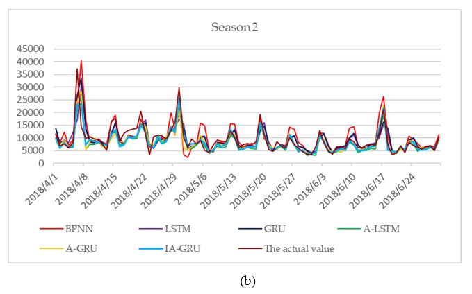
Sustainability 2020, 12, 1390                                                                       2 of 20

a difficult task, it has attracted attention in the literature. Developing a new forecasting technique is
necessary to obtain a satisfactorily accurate level.

1.1. Traditional Methods in Tourist Flow Forecasting
      In recent years, various studies on tourist flow forecasting have resulted in the development
of numerous forecasting methods. The early methods of tourist flow forecasting mainly include
econometric [2] and time-series models [3]. Econometric models mainly include autoregressive
distribution lag model [4], error correction model [5], and vector autoregressive model [6]. Time
series models mainly include autoregressive moving average model [7] and autoregressive integrated
moving average model [8,9]. These methods usually employ historical data to forecast future tourist
flow through a univariate or multivariate mathematical function, which depends mostly on linear
assumptions. These traditional methods have a good effect on tourist flow forecasting with linear
characteristics. However, the prediction effect of these models on complex nonlinear tourist flow
forecasting is inaccurate. Consequently, scholars have started to utilize machine-learning methods
to build nonlinear prediction models, such as support vector regression [10,11] and artificial neural
networks [12,13]. The artificial neural network methods have been used widely in tourist flow
forecasting. These methods emulate the processes of the human neurological system to process
self-learning from the historical tourist flow patterns, especially for nonlinear and dynamic variations.
Accurate predictions can be obtained through repeated training and learning to approximate the real
model. However, limitations are still observed in such methods, especially in addressing the sequence
dependence among input variables in time series prediction.

1.2. Improved Attention-based Gated Recurrent Unit Model in Tourist Flow Forecasting
      Recurrent Neural Network (RNN) is the most common and effective tool for time series models,
especially in addressing sequence dependencies among input variables [14]. In the calculation of RNN,
results are interdependent and the current input of the hidden layer is highly correlated with the
last output. However, as the time series progresses, the problem of gradient disappearance becomes
evident. To solve such a problem, a long short-time memory neural network (LSTM) [15] and Gated
Recurrent Unit (GRU) [16] are proposed based on the original RNN. GRU is an improved model of
LSTM, which controls the switch of memorizing and forgetting by setting multiple threshold gates.
LSTM and GRU solve the limitation problem of handling long-term dependencies well. These methods
have led to their successful application on various sequence learning problems, such as machine
translation [17], speech recognition [18], and load forecasting [19,20]. LSTM has also been applied
successfully for the first time in tourist flow forecasting [21]. In the study, LSTM was able to fit the
test datasets and was proved to be superior to autoregressive integrated moving average model and
backpropagation neural network, achieving the best performance in all cases. Therefore, LSTM and
GRU are the most advanced methods for addressing time series prediction problems. LSTM and GRU
can help capture long-term dependencies.
      However, their ability to process information is still insufficient. Learning from cognitive
neuroscience, researchers introduce attention mechanisms to the encoding–decoding framework [22,23]
to select further from the input series and encode the information in long-term memory to improve
information processing ability. In recent years, related works [24–26] on time series prediction are
improved usually by introducing attention layers into the encoding-decoding framework. The attention
mechanism has also been combined successfully with LSTM and applied to power forecasting [27],
load forecasting [28], and travel time forecasting [29]. However, few articles in tourist flow forecasting
have referred to this combined method. A cause of widespread concern is the work of Li et al. [30],
wherein the attention mechanism was combined with LSTM and competitive random search (CRS)
was used to configure the parameters of the attention layer, which improved the attention of LSTM
to varying degrees of sub-window features in multiple time steps. However, although the attention
mechanism improves the feature attention of LSTM in the time step, it remains insufficient for LSTM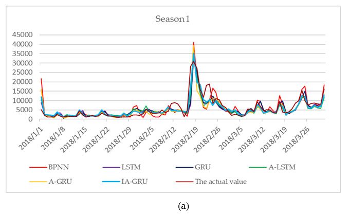
Sustainability 2020, 12, 1390                                                                         3 of 20

to pay different attention to sub-window features within different related factors. To solve such a
problem, this study changes the vertical weighting method based on time importance and proposes an
improved attention mechanism, which has horizontal weighting method based on factor importance.
This improved attention mechanism is trained with CRS and then combined with GRU to increase the
degree of attention of GRU to various related factors.

1.3. Web Search Index and Climate Comfort in Tourist Flow Forecasting
      In the study of tourist flow forecasting, the prediction accuracy of the model is affected by the
model itself and various factors. Moreover, existing studies have not considered other factors, such
as web search index and climate comfort. Given the rapid development of the internet, people can
easily search for information through search engines. At present, scholars believe that web search
is an important and advanced way to obtain timely data and useful information [31]. When using
the internet to search for data, the search history reflects the content of interest and the behavior that
follows. In recent years, web search data has provided a new source of data and analytical basis for
scientific research, which have been verified by researchers. For example, Choi and Varian have found
in their research on Hong Kong’s tourist flow forecasting that the autoregressive model including
Google search trends can improve prediction accuracy by at least 5% [32]. Prosper and Ryan have found
that Google search trends can significantly improve forecasting results in the tourist flow forecasting
studies on five tourist destinations in the Caribbean [33]. Similarly, Önder and Gunter have found
in the study of tourist flow forecasting in major European cities that the Google search index can
effectively improve the forecasting effect [34]. In view of various meteorological factors affecting tourist
flow, climate comfort has gradually become a hot spot and the focus of tourism-related research. Li et
al. have found in the tourism research on Hong Kong and other 13 major cities in China that climate
comfort has a significant positive impact on the tourist flow in the mainland [35]. Chen et al. have
included climate comfort in the model of Huangshan’s tourist flow forecasting and obtained better
prediction results, indicating that climate comfort is significantly correlated with daily tourist flow [36].
Therefore, in this study, the web search index and climate comfort are used as important factors in
tourist flow forecasting.
      This study aims to propose a tourist flow forecasting method based on web search index, climate
comfort, and Improved Attention-based GRU (IA-GRU) model. The CRS and attention mechanism
are used to optimize the attention layer. Then, the selected web search index and climate comfort
are added to improve the forecasting effect of IA-GRU model. The results of this study demonstrate
the effectiveness of this model. The remaining parts of this paper are organized as follows. Section 2
introduces the basic principles of LSTM, GRU, attention mechanism, and IA-GRU model. Section 3
presents the data-processing methods using Huangshan Scenic Area as the research subject. Section 4
discusses the prediction performance of the proposed model and the comparison with other basic
models. Section 5 provides the conclusion.

2. Methods
     In this section, we discuss the structure of LSTM and GRU and explain why GRU is chosen as
the prediction model. Then, we provide the outline for the attention mechanism and the details of
the IA-GRU model. In addition, we train the IA-GRU model with a collaborative mechanism, which
combines the attention mechanisms with CRS.

2.1. LSTM (GRU’s Precursor)
     LSTM is first proposed for language models in 1997 [15]. LSTM is an RNN with a special structure,
which has the advantage of being able to deal with the long-term dependency of time series. LSTM can
solve the problem of gradient disappearance caused by RNN after multi-level network propagation.
     As shown in Figure 1, one tanh layer σ and three layers exist inside LSTM. The three layers
correspond to three gates, namely, the forget gate, input gate, and output gate. The role of the horizontal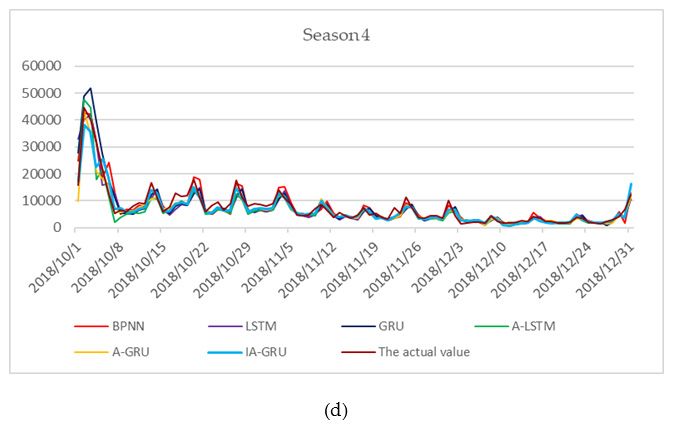
Sustainability 2020, 12, 1390 4 of 20
output gate.
Sustainability The
2020, 12, 1390role of the horizontal line is to pass ct −1 to ct . The three gates 4and
of 20
horizontal lines work together to complete the filtering and transmission processes
of input
line information.
is to pass ct−1 to ct . The three gates and horizontal lines work together to complete the filtering
and transmission processes of input information.
⊗ ⊕
⊗ ⊗
ct
Figure 1. Structure of long short-time memory neural network (LSTM).
Figure 1. Structure of long short-time memory neural network (LSTM).
We denote the input time series as xt , hidden state cells as st , and output sequence as ŷ. LSTM
neural
We networks perform
denote the input the computation
time series as xt ,as follows:
hidden state cells as st , and output sequence as ŷ . LSTM
neural networks perform the computation as follows:
ft = σ(w f · [st−1 , xt ] + b f ), (1)
ft = σ ( w f ⋅ [st −1 , xt ] + b f ) , (1)
it = σ(wi · [st−1 , xt ] + bi ), (2)
it = σ (wi ⋅ [st −1 , xt ] + bi ) , (2)
ct = tanh
e (wc · [st−1 , xt ] + bc ), (3)
ctct==tanh
ft ∗(w
ct−1
c
⋅ [+ c]t+
st −1it, x∗ te , bc ) , (4)
(3)
ot = σ(wo · [st−1 , xt ] + bo ), (5)
ct = ft ∗ ct −1 + it ∗ ct , (4)
st = ot ∗ tanh(ct ), (6)
σ (w
ot ŷ= = wyo ⋅·[sstt −+, x ] + bo ) ,
1 bty , (5)
(7)
where σ and tanh are activation functions applied st = otto∗ tanh
the internal
(ct ) , structure of LSTM. Equations (8) and
(6)
(9) are their calculation processes, respectively, wherein σ stands for the standard sigmoid function.
The output value of the σ layer is between 0 and 1. The output value determines whether the input
yˆ = wy ⋅ st + by , (7)
information can pass through the gate. A value of zero signifies “let nothing through,” whereas a value
of one means
where σ and“let
tanheverything through!”
are activation f , i, o,
functions and c respectively
applied to the internal denote the mentioned
structure of LSTM.inner-cell
Equationsgates,
(8)
namely, the forget gate, input gate, output gate, and cell activation vectors,
and (9) are their calculation processes, respectively, wherein σ stands for the standard sigmoidc should be equal to the
hidden
function.vector s. Thevalue
The output w terms denote
of the weight
σ layer matrices,0 whereas
is between and 1. The the b terms
output denote
value bias terms.
determines The
whether
input gate can determine how incoming vectors x alter the state of the memory
the input information can pass through the gate.t A value of zero signifies “let nothing through,” cell. The output gate
can allowathe
whereas memory
value of onecell to have
means “letan effect on the
everything outputs.f Then,
through!” , i , othe forget
, and gate allowsdenote
c respectively the cellthe
to
remember or forget its previous state.
mentioned inner-cell gates, namely, the forget gate, input gate, output gate, and cell activation
1
vectors, c should be equal to the hidden σvector (x) = s . The ,w terms denote weight matrices, whereas (8)
1 + e−x
the b terms denote bias terms. The input gate can determine how incoming vectors xt alter the state
ex − e−x
tanh(x) = x . (9)
e + e−xthe forget gate allows the cell to remember or forget its previous state.
1
σ ( x) = , (8)
1 + e−x
ex − e−x
Sustainability 2020, 12, 1390 tanh( x) = . (9)
5 of 20
ex + e−x
2.2.
2.2.GRU
GRU
Given
Giventhethecomplex
complexstructure
structureof
ofLSTM,
LSTM,the thetraining
trainingofofLSTM
LSTMRNNRNNoften
oftentakes
takesaalotlot of
of time.
time. To
To
improve
improvethethetraining
trainingspeed
speedand
andcapture
capturelong-term
long-termdependencies
dependenciesefficiently,
efficiently,GRU
GRUisisproposed
proposedas asan
an
improved
improvedmodel
modelofofLSTM
LSTMin in2014
2014due
dueto
toits
its simple
simplestructure
structure and
and easy
easy training
training [16].
[16]. The
Thestructure
structureofof
the
the GRU is shown in Figure 2. Unlike LSTM, GRU has only two gates, namely, reset gate r gate
GRU is shown in Figure 2. Unlike LSTM, GRU has only two gates, namely, reset r and
and update
gate z. gate z .
update
⊗ ⊕
⊗ ⊗s
t
Structureof
Figure2.2.Structure
Figure ofGated
GatedRecurrent
RecurrentUnit
Unit(GRU).
(GRU).
We denote the input time series as x , hidden state cells as st , and output sequence as ŷ. GRU
We denote the input time seriest as xt , hidden state cells as st , and output
neural networks perform the computation as follows:
sequence as ŷ . GRU neural networks perform the computation as follows:
rt = σ(wr · [st−1 , xt ]), (10)
rt = σ (wr ⋅ [st −1 , xt ]) , (10)
zt = σ(wz · [st−1 , xt ]), (11)
zt = σ (wz ⋅ [st −1 , xt ]) , (11)
st = tanh(w · [rt ∗ st−1 , xt ]),
e (12)
st s= = tanh(w ⋅ [rt ∗ s+t −1z,tx∗e
t (1 − zt ) ∗ st−1
])
t st ,, (13)
(12)
ŷ = w · s . (14)
st = (1 − zt ) ∗yst −1t + zt ∗ st , (13)
The reset gate r determines the proportion of the output state st−1 at the previous moment in the
new hidden state e st . The new hidden state e = w y ⋅ st . by performing a nonlinear transformation
st isyˆ obtained (14)
of the tanh activation function on the output state at the previous moment st−1 and the input at the
current moment xt . The update gate z mainly affects the proportion of the current hidden state st in the
new hidden state e st . Concurrently, the update gate z controls the proportion of e st and st−1 in the final
output state st .
2.3. Attention Mechanism
When observing a scene in the real world, humans typically focus on certain fixation point at first
glance. Their attention is always concentrated on a certain part of the focus. The human visual attentionhidden state st in the new hidden state st . Concurrently, the update gate z controls the proportion
of st and st −1 in the final output state st .
2.3. Attention Mechanism
Sustainability 2020, 12, 1390 6 of 20
When observing a scene in the real world, humans typically focus on certain fixation point at
first glance. Their attention is always concentrated on a certain part of the focus. The human visual
mechanism is a model
attention mechanism is aofmodel
resource allocation,
of resource providing
allocation, different
providing attention
different to different
attention areas.areas.
to different The
attention mechanism
The attention is proposed
mechanism by imitating
is proposed the principle
by imitating the of human vision’s
principle of human attention distribution;
vision’s attention
then, the attention
distribution; mechanism
then, the attentionismechanism
combined with the encode–decode
is combined framework [22]
with the encode–decode to complete
framework [22]the
to
process
complete of the
attention
processchange. The focus
of attention of thisThe
change. study is toof
focus assign different
this study is attention
to assign weights
differentto attention
different
related
weightsfactors through
to different the attention
related mechanism
factors through and continuously
the attention mechanism optimize the weightsoptimize
and continuously to improve the
the prediction
weights effect ofthe
to improve theprediction
model. Theeffect
attention
of themechanism
model. Theattached to themechanism
attention encode–decode framework
attached to the
is exhibited in Figure
encode–decode 3 (see Section
framework 2.4 for
is exhibited in details).
Figure 3 (see Section 2.4 for details).
Figure 3.
Figure 3. Attention mechanism.
Attention mechanism.
Figure 33illustrates
Figure illustrates
howhow the attention
the attention mechanismmechanism is combined
is combined with the encode–decode
with the encode–decode framework.
We attach attention
framework. We attach weights
attention ,W2 , . . . ,W
W1weights Wn1 ,to
W2input
,…, Wvariables x1 ,x2 , . . . ,xxn1,, transform
n to input variables x2 ,…, xn , transform
the attention
the
weights into intermediate semantics C 1 ,C2 , . . . ,Cn through encoding,
attention weights into intermediate semantics C1 , C 2 ,…, Cn through encoding, and then transformand then transform the
intermediate semantics into new attention weights W1 0 ,W2'0 , . . .' ,Wn 0 through decoding.
the intermediate semantics into new attention weights W1 , W2 ,…, Wn ' through decoding.
2.4. IA-GRU Model
2.4. IA-GRU Model
When the GRU model constructs tourist flow forecasting, the entire training process is continuously
When
learning andthe GRU model
memorizing the constructs tourist related
effects of various flow forecasting,
factors on thethetarget
entirevalue.
training
Theprocess
proposed is
continuously learning and memorizing the effects of various related factors on
IA-GRU model in this study combines the attention mechanism with GRU. On the basis of the ability of the target value. The
proposed
GRU IA-GRU
to handle timemodel
series in this study
prediction combinesthe
problems, theIA-GRU
attention mechanism
model with GRU.
assigns different On the weights
attention basis of
the ability of GRU to handle time series prediction problems, the IA-GRU model
to different related factors and continuously optimizes them to improve the learning and generalization assigns different
attentiontoweights
abilities achieve theto different
purpose of related factors
improving theand continuously
prediction effect ofoptimizes
the model.them to improve the
learning and4 generalization
Figure consists of twoabilities to achieve
parts. The left partthe purpose
shows the of improving
process of GRUthemodeling
predictionandeffect of the
training,
model.
whereas the right part shows the process of attention mechanism with CRS to optimize attention
Figure
weights. 4 consists
In the left part,ofwe
two parts.
obtain theThe leftdata.
input part Then,
showswe theadd
process of GRUlayer
an attention modeling
to GRUand training,
on the basis
whereas
of the right
how human part
vision shows the
processes process
input of attention
information throughmechanism withmechanism.
the attention CRS to optimize attention
The introduced
weights. In
attention the left part,
mechanism can we obtain the attach
quantitatively input data.
weights Then, we addfactors
to related an attention layer toimportance
with different GRU on the to
basis of how human vision processes input information through the attention
avoid distraction. Finally, the weighted input data is sent to the GRU layers to obtain the predicted mechanism. The
introduced
value. attention mechanism
The prediction can quantitatively
error is also calculated. Moreover, attach weights toerrors
the predicted related
arefactors
regarded with different
as feedback
and sent to direct the process of optimizing attention weights. In the right part, the randomly generated
attention weights set is binary encoded. Then, the champion attention weights subset is selected
according to the error feedback, and the new attention weights are reconstructed. Finally, the updated
attention weights set is decoded, whereas the optimal attention weights are sent to the attention layer.the predicted value. The prediction error is also calculated. Moreover, the predicted errors are
regarded as feedback and sent to direct the process of optimizing attention weights. In the right part,
the randomly generated attention weights set is binary encoded. Then, the champion attention
weights subset is selected according to the error feedback, and the new attention weights are
Sustainability 2020,Finally,
reconstructed. 12, 1390 the updated attention weights set is decoded, whereas the optimal attention
7 of 20
weights are sent to the attention layer.
Figure GRU
4. 4.
Figure training
GRU process
training based
process on on
based attention mechanism
attention with
mechanism competitive
with random
competitive search
random (CRS).
search
(CRS).
The concrete steps of the modeling and training of GRU and the combined attention mechanism
and CRS used to optimize the attention weights are presented as follows:
The concrete steps of the modeling and training of GRU and the combined attention mechanism
(1) Modeling and training of GRU
and CRS used to optimize the attention weights are presented as follows:
Step 1: n columns of input data are obtained, corresponding to n related factors: xt =
(1) Modeling and training of GRU
(xt , x2t , . . . , xnt ).
1
Step 1: n columns of input data are obtained, corresponding to n related factors:
Step 2: attention weights are defined: Wi = (Wi1 , Wi2 , . . . , Win ).
xt = ( xt1 , xt2 ,..., xtn ) .
Step 3: the input data are weighed at the attention layer: e xt = (x1t Wi1 , x2t Wi2 , . . . , xnt Win ).
Step
Step 4: e 2: attention weights are defined: W = ( W
xt is sent to GRU neural networksi to acquirei
1
, W 2
,..., W
i the finali ) . predicted value.
n
Step 3: the input
(2) Combined data aremechanism
attention weighed atandthe CRS
attention x t = ( xt1Wweights
layer: attention
optimizing i , xt Wi ,..., xt Wi ) .
1 2 2 n n
Step 4: x t is
According to sent
the genetic
to GRU algorithm, the purpose
neural networks of CRS
to acquire is to predicted
the final generate the optimal parameter
value.
combination in the attention layer. The process of CRS is elaborated in Figure 4. CRS comprises four
(2) Combined attention mechanism and CRS optimizing attention weights
parts, which are introduced as follows:
According to the genetic algorithm, the purpose of CRS is to generate the optimal parameter
In Figure 4, attention weights set W is provided in “A,” while being translated into W B through
combination in the attention layer. The process of CRS is elaborated in Figure 4. CRS comprises four
binary code in “B.” The subset Wi denotes attention weights and is transferred into GRU neural
parts, which are introduced as follows:
networks in the left part, wherein it produces a corresponding loss value according to a predicted error
In Figure 4, attention weights set W is provided in “A,” while being translated into W B
in the networks. Then, the champion attention weights subsets WiB and WiB are selected according
through binary code in “B.” The subset Wi denotesisattention
to the loss of W B in “C,” and its subset combination
weights and is transferred into GRU
traversed repeatedly. Finally, a new attention
neural
weight networks in the
WkB is rebuilt left The
in “D.” part,three
wherein it produces
random operators aincorresponding
the dotted box loss value according
are introduced to a
to illustrate
B
how Wk is rebuilt.Sustainability 2020, 12, 1390 8 of 20
The concrete steps of CRS are stated as follows:
Step 1: attention weights set of size M = 36 are randomly generated: W = (W1 , W2 , . . . , Wi , . . . WM ).
Step 2: subset Wi is sent to the attention layer, whereas W is binary encoded: W B =
(W1 , W2B , . . . , WiB , . . . , WM
B B ).
Step 3: the prediction error is calculated based on the true value y and the predicted value ŷ from
the GRU model: Loss( ŷ(W ), y).
Step 4: according to the error feedback, the champion attention weights subsets WiB and W Bj are
selected. Each subset comprises binary strings and is evenly divided into n segments, where n is
the number of related factors mentioned in the first part of this section. Correspondingly, WiB and
W Bj are represented by WiB = (F1i , F2i , . . . , Fni ) and W Bj = (F1j , F2j , . . . , Fnj ). F1i and F1j are part of WiB and
W Bj , respectively.
Step 5: the segments of WiB and W Bj are randomly selected. For instance, segment n-1 of the two is
selected, that is, Fn−1
i
and Fn−1
j
. However, the number of selected subsections is not fixed.
Step 6: genetic recombination of Fn−1i
and Fn−1
j
are obtained. Fn−1i
and Fn−1
j
are represented by
binary codes with a length of six, and the two are randomly exchanged on the corresponding six indices
to obtain the recombined segment Fn−1 k
. For example, Fn−1
i
= (0, 1, 0, 0, 1, 1) and Fn−1
j
= (1, 0, 1, 0, 0, 1)
are exchanged on the odd index to obtain Fn−1 k
= (1, 1, 1, 0, 0, 1). The indices where actual exchanges
transpire are decided randomly.
Step 7: a genetic mutation is imitated and the genotype of Fn−1 k
is reversed. For instance, 0 is
reversed to 1. Then, Fn−1 k
= ( 0, 0, 0, 1, 1, 0 ) replaces the corresponding F n−1 in W B , forming W B that is
i i k
inserted into W B .
Step 8: W B is decoded to acquire the updated attention weights set: W0 =
( W1 0 , W2 0 , . . . , Wk 0 , . . . , WM 0 ) .
Step 9: Steps 2–8 above should be repeated until the preset number of epochs is reached.
The entire process from the selection of input data to the training and optimization of the IA-GRU
model is shown in Figure 5 (see Section 3 for concrete steps for selecting input data).Sustainability 2020, 12, 1390 9 of 20
Sustainability 2020, 12, 1390 9 of 20
Figure 5.
Figure 5. The
The flowchart.
flowchart.
3. Data Preparation
This study takes the Huangshan Scenic Area as an example
example of a famous Chinese
Chinese scenic
scenic spot.
spot.
Huangshan is listed as one of UNESCO world natural and cultural heritage sites in 1990. Moreover,
Moreover,
Huangshan has been selected as one of the first global geoparks in 2004. A total of 3.38 million local
and foreign tourists have visited Huangshan in 2018.Sustainability 2020, 12, 1390 10 of 20
Huangshan has been selected as one of the first global geoparks in 2004. A total of 3.38 million local
and foreign tourists have visited Huangshan in 2018.
In this study, we use the daily historical data of the Huangshan Scenic Area from 2014 to 2018 as
experimental data. The data includes (1) Basic data: the total number of tourists in the past, target total
number of tourists, number of online bookings, weather, official holiday, and weekends; (2) the Baidu
index of keywords: Huangshan, Huangshan weather, Huangshan tourism guide, Huangshan tourism,
Huangshan scenic area, Huangshan tickets, Huangshan first-line sky, Anhui Huangshan, Huangshan
weather forecast, and Huangshan guide; (3) climate comfort: composed of average temperature,
average relative humidity, and average wind speed. The data (1) is obtained from a research project
in cooperation with the Huangshan scenic area. The data (2) is obtained from Baidu Index Big Data
Sharing Platform (http://index.baidu.com/v2/index.html?from=pinzhuan#/). The data (3) is obtained
from the China Meteorological Data Network (http://data.cma.cn/).
3.1. Basic Data
To learn as many data features and tourist flow rules as possible, the data from 2014 to 2017 were
selected as the training set and the data from 2018 were selected as the test set.
(1) Total number of tourists in the past
The total number of tourists in the past is selected as one of the related factors of the prediction
model, given that the annual and even daily tourist flow shows a certain regularity. The impact of past
tourist flow on the current tourist flow may have a lag period. Thus, a correlation analysis was made
between the past total number of tourists with different lag periods and the target total number of
tourists. In this study, the maximum lag period was two years. Based on previous experience, the total
number of tourists in the past with a correlation index greater than 0.440 was selected as the input
variable. Table 1 shows the correlation analysis results with a confidence level of 0.01.
Table 1. Correlation analysis results of the total number of people.
Lag Period 0 1 2 3 4 5 6 7 ...
Correlation 1.000 0.718 0.443 0.324 0.243 0.197 0.256 0.341 ...
Lag Period 365 366 367 368 369 370 371 372 ...
Correlation 0.522 0.350 0.280 0.212 0.147 0.187 0.267 0.201 ...
Therefore, the total number of tourists in the past with a lag period of one day, two days, and
365 days were selected as the input variables, that is, the total number of tourists yesterday x1 , the
total number of tourists the day before yesterday x2 , and the total number of tourists on the day of last
year x3 .
(2) Number of online bookings
Given the internet’s rapid growth, its impact on people’s lifestyles is increasingly evident. Online
operations are becoming persistently convenient. To a great extent, the number of online bookings can
reflect the trend of the total number of tourists. Therefore, the number of online bookings was selected
as the input variable x4 .
(3) Weather
The weather is the decisive factor for outbound tourism, wherein the weather is either good or bad
for tourists. Therefore, the weather is selected as the input variable x5 in the form of a dummy variable:
x5 = { 01 , where 0 represents non-severe weather, such as sunny, cloudy, and drizzle; 1 represents
severe weather, such as moderate rain, heavy rain, moderate snow, heavy snow, and blizzard.
(4) Official holiday
Traveling on holidays is a common phenomenon. Whenever a holiday arrives, the number of
tourists in famous scenic spots consistently soars. Therefore, holidays were selected as input variable
x6 in the form of a dummy variable:Sustainability 2020, 12, 1390 11 of 20
x6 = { 01 , where 0 indicates an ordinary day; 1 indicates official holiday.
(5) Weekend
A week cycle comprises seven days. Monday to Friday is weekdays and Saturday and Sunday
are rest days. Going out and traveling on rest days are common phenomena. Therefore, the weekend
was selected as the input variable x7 in the form of a dummy variable:
x7 = { 01 , where 0 represents a working day; 1 represents the rest of the day.
3.2. Baidu Index of Keywords
Baidu is the largest search engine in China and has the most users. When searching for
consumer behavior in China, Baidu search has higher predictive power than Google search [37].
This study selects the keywords that tourists commonly use in the Baidu search engine to search
the key analysis object. We search for the keyword “Huangshan” in Baidu’s keywords-mining tool
(http://stool.chinaz.com/baidu/words.aspx), and find the top-10 keywords related to Huangshan in the
top 100 rankings, namely, Huangshan, Huangshan weather, Huangshan tourism guide, Huangshan
tourism, Huangshan scenic area, Huangshan tickets, Huangshan first-line sky, Anhui Huangshan,
Huangshan weather forecast, and Huangshan guide. Considering that the Baidu search has a lagging
effect on tourist flow, a correlation analysis between the above Baidu index of keywords with different
lag periods and the target total number of tourists is performed. Similarly, the maximum lag period is
two years. Accordingly, the Baidu index of keywords with a correlation index greater than 0.440 is
selected as input variable. The analysis results are shown in Tables 2 and 3.
Table 2. Correlation analysis results of the top five keywords.
Huangshan Huangshan Huangshan Huangshan
lag Period Huangshan
Weather Tourism Guide Tourism Scenic Area
0 0.510 0.107 0.523 0.107 0.330
1 0.552 0.180 0.597 0.206 0.367
2 0.556 0.236 0.614 0.281 0.356
3 0.491 0.221 0.569 0.278 0.299
4 0.432 0.198 0.510 0.262 0.242
5 0.393 0.178 0.462 0.241 0.202
6 0.330 0.146 0.411 0.160 0.172
7 0.280 0.125 0.374 0.115 0.150
... ... ... ... ... ...
365 0.322 0.099 0.350 0.170 0.156
366 0.363 0.118 0.396 0.236 0.183
367 0.376 0.123 0.413 0.259 0.185
368 0.362 0.118 0.404 0.259 0.165
369 0.346 0.115 0.385 0.246 0.144
370 0.292 0.098 0.337 0.171 0.115
371 0.244 0.089 0.298 0.124 0.086
372 0.253 0.106 0.293 0.170 0.085Sustainability 2020, 12, 1390 12 of 20
Table 3. Correlation analysis results of the last five keywords.
Huangshan Huangshan Anhui Huangshan Huangshan
lag Period
Tickets First-Line Sky Huangshan Weather Forecast Guide
0 0.232 0.209 0.372 0.188 0.354
1 0.281 0.198 0.462 0.324 0.463
2 0.275 0.184 0.542 0.420 0.500
3 0.243 0.166 0.527 0.397 0.473
4 0.217 0.147 0.489 0.354 0.426
5 0.209 0.135 0.455 0.329 0.383
6 0.195 0.128 0.376 0.272 0.301
7 0.153 0.118 0.312 0.239 0.237
... ... ... ... ... ...
365 0.206 0.114 0.260 0.199 0.158
366 0.208 0.114 0.322 0.261 0.241
367 0.194 0.112 0.355 0.280 0.258
368 0.184 0.106 0.362 0.264 0.255
369 0.182 0.102 0.356 0.260 0.244
370 0.168 0.097 0.301 0.212 0.190
371 0.152 0.089 0.253 0.178 0.146
372 0.135 0.081 0.273 0.218 0.167
As shown in Tables 2 and 3, the Baidu index of keyword with a lag period of two days has
the highest correlation with the actual total number of tourists. Thus, we chose the Baidu index of
Huangshan, Huangshan tourism guide, Anhui Huangshan, and Huangshan guide with a lag period of
two days as input variables x8 , x9 , x10 , and x11 , respectively.
3.3. Climate Comfort
Climate comfort is an important environmental factor that affects tourists’ travel. Therefore, we
select climate comfort as the input variable x12 . Climate comfort is the climatic condition in which
people can maintain the normal physiological process and feel comfortable without any help of heat
and cold [38]. The degree of human comfort is closely related to meteorological conditions, which
are the comprehensive feeling of temperature, humidity, and wind in the meteorological field. The
equation for calculating climate comfort is presented as follows [39]:
Q = 1.8t − 0.55(1.8t − 26)(1 − h) − 3.25v + 32. (15)
In Equation (15), t is the average temperature (◦ C), h is the average relative humidity (%), v is the
average wind speed (m/s), and Q is the climate comfort.
4. Experiments and Results
4.1. Building IA-GRU Model
In the IA-GRU model, except for the attention layer, parameters used in GRU neural networks
can be learned by standard backpropagation through time algorithm with mean squared error as the
objective function. According to previous experience and the results of repeated experiments, the
IA-GRU model has six layers, namely, one attention layer, four GRU layers, and one fully connected
layer. Moreover, the total number of neurons in four GRU layers was 128, 64, 64, and 32, respectively.
The activation function of the fully connected layer is the Scaled Exponential Linear Units function.
The number of training epochs in GRU layers is 500, and the mini-batch size of the training dataset is
64. According to the results of trial and error, the number of epochs in CRS was 15. Therefore, the
IA-GRU model has been established in this study.Sustainability 2020, 12, 1390 13 of 20
4.2. Results and Discussion
The proposed IA-GRU model is compared with some basic models, such as Back Propagation
Neural Network (BPNN), LSTM, GRU, Attention-LSTM (A-LSTM), and Attention-GRU (A-GRU). The
dataset of the IA-GRU model and basic models includes basic data x1 –x7 , Baidu index of keywords
(1–4 keywords) x8 –x11 , and climate comfort x12 . To evaluate the predictive performance of each model,
we choose the average absolute percentage error (MAPE) and the correlation coefficient (R) as the
evaluation indicators. MAPE represents the prediction error, and R represents the degree of correlation
between the predicted value and the true value. The smaller the MAPE, the smaller the deviation
between the predicted value and the true value; the closer R is to 1, the higher the degree of correlation
between the predicted value and the true value. The equations are presented as follows:
n
1 X yi − ŷi
MAPE = ( | |) × 100, (16)
n yi
i=1
n
P
yi ŷi
i=1
R= s s . (17)
n n
2 2
P P
yi ŷi
i=1 i=1
In the equations, yi represents the true value and ŷi represents the predicted value.
In this section, we apply the data x1 –x12 to IA-GRU model and basic models to testify the validity
of the IA-GRU model on tourist flow forecasting. The overall experimental results are shown in
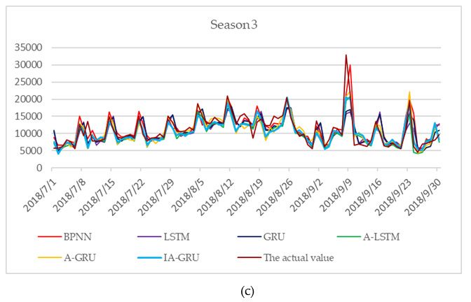
Table 4, and the daily true and predicted values are shown in Figure 6. IA-GRU model with MAPE
was lower than the others and R is higher than the others, which signifies that the prediction effect of
the IA-GRU model is better than the abovementioned basic models. With regard to MAPE, IA-GRU
was 7.77% lower than BPNN, in which MAPE was the highest. With regard to R, IA-GRU was 0.0299
higher than BPNN, in which R was the lowest. Furthermore, by comparing IA-GRU with A-GRU,
we found that the former had a lower MAPE and a higher R, which indicates that the improved
attention mechanism proposed in this study played a significant role. By comparing GRU with LSTM
or comparing A-GRU with A-LSTM, the results show that the prediction effect of GRU was better than
that of LSTM. However, R of the A-GRU model is lower than the R of the A-LSTM model. BPNN was
not chosen in this area given that its MAPE was too high for forecasting at 28.58%. In summary, the
IA-GRU model had the best prediction effect.
Table 4. Experimental results of different models.
Models MAPE(%) R
IA-GRU 20.81 0.9761
A-GRU 21.71 0.9674
A-LSTM 22.87 0.9711
GRU 25.43 0.9547
LSTM 25.57 0.9480
BPNN 28.58 0.9462Sustainability 2020, 12, 1390 14 of 20
Sustainability 2020, 12, 1390
LSTM 25.57 0.9480 14 of 20
BPNN 28.58 0.9462
Figure 6. Cont.Sustainability 2020, 12, 1390 15 of 20
Sustainability 2020, 12, 1390 15 of 20
Figure 6. The
Theactual
actualand
andpredicted
predictedvalues
valuesofof2018.
2018.(a)(a)
The actual
The and
actual predicted
and values
predicted of season
values 1; (b)
of season 1;
the actual and predicted values of season 2; (c) the actual and predicted values of season
(b) the actual and predicted values of season 2; (c) the actual and predicted values of season 3; (d) the
predicted values
actual and predicted values of
of season
season 4.
4.
To
To further
further verify
verify the
the prediction
prediction effect
effect of
of the
the IA-GRU
IA-GRU model,
model, the comparative experiments
experiments in this
study were divided into four categories, that is, the prediction results of different models models including
including
datasets 1, 2, 3,
3, and
and 4.4. Dataset
Dataset11contains
containsbasic
basicdata,
data,dataset
dataset2 2contains
contains basic data and Baidu
basic data and Baidu index index
of
of keywords
keywords (4 (4 keywords),
keywords), dataset3 3contains
dataset containsbasic
basicdata
dataand
andclimate
climatecomfort,
comfort, and
and dataset
dataset 4 contains
basic data, Baidu index of keywords, and climate climate comfort.
comfort. Dataset 4 is the dataset mentioned in the
previous
previous paragraph.
paragraph.
Tables
Tables5–95–9exhibit
exhibit thethe
experimental
experimental results of different
results models
of different including
models datasetsdatasets
including 1–4. The1–4.
increase
The
in keywords in Tables 6 and 7 is in accordance with the correlation index in Section
increase in keywords in Tables 6–7 is in accordance with the correlation index in Section 3.3 from 3.3 from high to
low.
high The results
to low. Theshow that
results morethat
show keywords make the make
more keywords prediction more accurate.
the prediction moreAs shown in
accurate. AsTables
shown5–9,in
the prediction
Tables 5–9, theeffect of IA-GRU
prediction model
effect is bettermodel
of IA-GRU than the other basic
is better than models on basic
the other each dataset,
models wherein
on each
the predicted
dataset, wherein value
the had a higher
predicted correlation
value had a higherwithcorrelation
the real value.
with theIn the
realfour datasets,
value. the datasets,
In the four IA-GRU
model had the
the IA-GRU lowest
model had MAPE on dataset
the lowest MAPE 4 and
on the highest
dataset R, which
4 and signifies
the highest that the
R, which Baidu index
signifies of
that the
keywords
Baidu index and
of climate
keywords comfort furthercomfort
and climate improvefurther
prediction accuracy.
improve prediction accuracy.
Table 5. The results with
Table 5. with dataset
dataset 1.
1.
Models
Models MAPE(%)
MAPE(%) RR
IA-GRU
IA-GRU 22.43
22.43 0.9736
0.9736
A-GRU 24.55 0.9696
A-GRU
A-LSTM 24.55
25.46 0.9696
0.9660
GRU
A-LSTM 27.36
25.46 0.9494
0.9660
LSTM 27.91 0.9659
GRU
BPNN 27.36
30.17 0.9494
0.9460
LSTM 27.91 0.9659
BPNN 30.17 0.9460
Table 6. The results with dataset 2.
MAPE(%)
Models
One Keyword Two Keywords Three Keywords Four Keywords
IA-GRU 22.34 22.04 22.40 21.33
A-GRU 23.74 23.68 23.19 23.54
A-LSTM 24.59 24.38 24.09 23.89Sustainability 2020, 12, 1390 16 of 20
Table 6. The results with dataset 2.
MAPE(%)
Models
One Keyword Two Keywords Three Keywords Four Keywords
IA-GRU 22.34 22.04 22.40 21.33
A-GRU 23.74 23.68 23.19 23.54
A-LSTM 24.59 24.38 24.09 23.89
GRU 27.16 25.86 24.99 25.54
LSTM 27.43 27.40 27.66 26.78
BPNN 29.81 29.87 29.24 28.78
Table 7. The results with dataset 2.
R
Models
One Keyword Two Keywords Three Keywords Four Keywords
IA-GRU 0.9677 0.9707 0.9720 0.9761
A-GRU 0.9644 0.9673 0.9713 0.9678
A-LSTM 0.9678 0.9740 0.9662 0.9736
GRU 0.9533 0.9563 0.9517 0.9532
LSTM 0.9688 0.9485 0.9724 0.9725
BPNN 0.9464 0.9397 0.9445 0.9528
Table 8. The results with dataset 3.
Models MAPE(%) R
IA-GRU 21.48 0.9688
A-GRU 22.67 0.9663
A-LSTM 23.89 0.9766
GRU 25.62 0.9538
LSTM 26.89 0.9504
BPNN 28.86 0.9542
Table 9. The results with dataset 4.
Models MAPE(%) R
IA-GRU 20.81 0.9761
A-GRU 21.71 0.9674
A-LSTM 22.87 0.9711
GRU 25.43 0.9547
LSTM 25.57 0.9480
BPNN 28.58 0.9462
To further analyze the prediction accuracy of the IA-GRU model, we performed a monthly analysis
of the experimental results of different models using dataset 4, as shown in Tables 10 and 11. As shown
in Table 10, the annual average error of the IA-GRU model was lower than that of basic models, whereas
the error of all models from May to October is lower than the annual average error. In May, June, and
July, the error of the IA-GRU model was lower than that of basic models. All models exhibited high
errors in January, February, March, April, and December. One of the reasons may be that they were
in the off-peak period. Moreover, the actual value is small, which is likely to cause high numerical
deviations. Overall, the IA-GRU model is relatively stable. In February, April, May, June, July, and
November, the IA-GRU model had the lowest error. Although the prediction of the IA-GRU model
was not the best in other months of the year, it was not the worst. For example, the error in January
was 8.48% higher than the minimum error, but 10.44% lower than the maximum error. The errors in
March, September, and October were close to the minimum error, wherein the gap between the errorSustainability 2020, 12, 1390 17 of 20
and the minimum error in these three months is less than 2%. The performance of IA-GRU model in
December was similar to that in January. IA-GRU model had the largest error in August, which was
2.22% higher than the lowest error. In August, the gap between the two errors is relatively small. The
reason may be that a certain gap exists in the correlation index of the Baidu index between the training
and test sets. Through correlation analysis, as shown in Table 12, we find that the correlation index of
the Baidu index of the training set is low, but the correlation index of the Baidu index of the test set is
high, which may cause a certain bias in the feature learning of the Baidu index. As shown in Table 11,
the R of the IA-GRU model was the highest in January, February, April, May, and November, and the R
from January to December was greater than 0.95. Such values are closely related to the annual average
R. Thus, the IA-GRU model was relatively stable, compared to other models.
Table 10. The monthly analysis results with dataset 4.
MAPE(%)
Months
IA-GRU A-GRU A-LSTM GRU LSTM BPNN
1 40.86 32.38 48.92 41.85 40.28 51.30
2 30.73 35.58 38.16 37.47 35.41 46.67
3 25.82 27.82 23.95 29.35 29.18 32.32
4 23.26 26.88 26.95 27.97 30.16 29.25
5 13.72 17.56 17.67 21.45 23.44 33.58
6 14.25 14.27 15.84 18.7 18.34 24.52
7 12.53 14.51 13.27 14.86 16.96 13.55
8 13.38 13.36 11.94 11.71 11.74 11.16
9 18.51 17.03 18.25 23.60 24.48 26.94
10 18.27 17.62 23.14 29.84 30.13 28.15
11 14.17 16.26 16.68 18.11 21.62 21.22
12 24.82 28.24 20.74 30.93 25.79 25.63
Average 20.81 21.71 22.87 25.43 25.57 28.58
Table 11. The monthly analysis results with dataset 4.
R
Months
IA-GRU A-GRU A-LSTM GRU LSTM BPNN
1 0.9538 0.8650 0.9502 0.9132 0.9506 0.8226
2 0.9546 0.9219 0.9443 0.9270 0.9226 0.8804
3 0.9779 0.9751 0.9803 0.9554 0.9498 0.9585
4 0.9673 0.9447 0.9557 0.9309 0.9070 0.9054
5 0.9880 0.9808 0.9823 0.9648 0.9581 0.9348
6 0.9915 0.9895 0.9917 0.9698 0.9682 0.9788
7 0.9845 0.9810 0.9852 0.9764 0.9723 0.9878
8 0.9912 0.9890 0.9938 0.9913 0.9912 0.9918
9 0.9685 0.9709 0.9675 0.9390 0.9319 0.9496
10 0.9860 0.9875 0.9750 0.9718 0.9580 0.9725
11 0.9842 0.9802 0.9806 0.9714 0.9609 0.9685
12 0.9549 0.9582 0.9663 0.9402 0.9459 0.9529
Average 0.9761 0.9674 0.9711 0.9547 0.9480 0.9462
Table 12. Correlation analysis results of keywords in August.
Huangshan Huangshan Travel Guide Anhui Huangshan Huangshan Guide
Training set 0.295 0.445 0.225 0.275
Test set 0.478 0.656 0.061 0.321
In summary, the proposed IA-GRU model based on the Baidu index and climate comfort can
effectively improve the accuracy of tourist flow forecasting. Moreover, the model proposed in thisSustainability 2020, 12, 1390 18 of 20
study is generally better than other basic models, proving the effectiveness of the model in tourist
flow forecasting.
5. Conclusions
This study proposes IA-GRU model trained with CRS for accurate tourist flow forecasting.
Tourism is an important part of the local, national, and global economies. Thus, good predictive
models are becoming increasingly valuable in tourist destinations management. First, this study is
the first to apply GRU in the field of tourist flow forecasting, wherein an attention layer is added
into GRU neural networks. Then, an improved attention mechanism that weighs different related
factors is proposed. Finally, the improved attention mechanism is combined with GRU, and CRS is
used to generate the optimal parameter combination at the attention layer. As a result, the IA-GRU
model captures long-term dependencies and increases the degree of attention that GRU pays to the
characteristics of sub-windows in different related factors. Concurrently, this study also explores the
application of the Baidu index and climate comfort in prediction models. In selecting the Baidu index
of keywords, Baidu’s keywords-mining tools and correlation analysis methods are used to screen out
relevant keywords with a large correlation index. In synthesizing climatic comfort, the comprehensive
sensation of temperature, humidity, and wind speed in the meteorological field is considered, and
the corresponding climatic comfort is calculated. This study takes the famous Huangshan Scenic
Area as an example to verify the effectiveness of the IA-GRU model with the Baidu index and climate
comfort in tourist flow forecasting. The experimental results prove that the IA-GRU model with the
Baidu index and climate comfort has higher prediction accuracy in tourist flow forecasting than basic
models. Thus, the proposed model can help the administration department in managing the scenic area
efficiently. Although this study has certain limitations, it remains worthy of further study in the future.
For example, a more detailed method of dividing weather dummy variables, a more accurate method
of keywords selection, and a more accurate method of climate comfort calculation can be explored in
future studies. In general, the proposed IA-GRU model is highly suitable for tourist flow forecasting.
Overall, the proposed model provides a significant reference for tourist destinations management and
a new perspective for related research.
Author Contributions: Data curation, W.L. and J.J.; formal analysis, W.L. and J.J.; methodology, W.L. and J.J.;
supervision, B.W., K.L., C.L., J.D. and S.Z.; writing—original draft, W.L. and J.J. All authors have read and agreed
to the published version of the manuscript.
Funding: This research received no external funding.
Acknowledgments: This work was supported by the National Natural Science Foundation of China (NSFC)
(71331002, 71771075, 71771077, 71601061) and supported by “the Fundamental Research Funds for the Central
Universities” (PA2019GDQT0005).
Conflicts of Interest: The authors declare no conflict of interest.
References
1. Wang, J. Anhui Statistical Yearbook; China Statistics Publishing House: Beijing, China, 2017.
2. Li, G.; Song, H.; Witt, S.F. Recent developments in econometric modeling and forecasting. J. Travel Res. 2005,
44, 82–99. [CrossRef]
3. Burger, C.; Dohnal, M.; Kathrada, M.; Law, R. A practitioners guide to time-series methods for tourism
demand forecasting—A case study of Durban, South Africa. Tour. Manag. 2001, 22, 403–409. [CrossRef]
4. Croes, R.R.; Vanegas, M., Sr. An econometric study of tourist arrivals in Aruba and its implications.
Tour. Manag. 2005, 26, 879–890. [CrossRef]
5. Daniel, A.C.M.; Ramos, F.F. Modelling inbound international tourism demand to Portugal. Int. J. Tour. Res.
2002, 4, 193–209. [CrossRef]
6. Witt, S.F.; Song, H.; Wanhill, S. Forecasting tourism-generated employment: The case of denmark. Tour. Econ.
2004, 10, 167–176. [CrossRef]Sustainability 2020, 12, 1390 19 of 20
7. Chu, F.-L. Forecasting tourism demand with ARMA-based methods. Tour. Manag. 2009, 30, 740–751.
[CrossRef]
8. Gil-Alana, L. Modelling international monthly arrivals using seasonal univariate long-memory processes.
Tour. Manag. 2005, 26, 867–878. [CrossRef]
9. Chen, C.-F.; Chang, Y.-H.; Chang, Y.-W. Seasonal ARIMA forecasting of inbound air travel arrivals to Taiwan.
Transportmetrica 2009, 5, 125–140. [CrossRef]
10. Chen, K.-Y.; Wang, C.-H. Support vector regression with genetic algorithms in forecasting tourism demand.
Tour. Manag. 2007, 28, 215–226. [CrossRef]
11. Hong, W.-C.; Dong, Y.; Chen, L.-Y.; Wei, S.-Y. SVR with hybrid chaotic genetic algorithms for tourism demand
forecasting. Appl. Soft Comput. 2011, 11, 1881–1890. [CrossRef]
12. Benardos, P.; Vosniakos, G.-C. Optimizing feedforward artificial neural network architecture. Eng. Appl.
Artif. Intell. 2007, 20, 365–382. [CrossRef]
13. Law, R.; Au, N. A neural network model to forecast Japanese demand for travel to Hong Kong. Tour. Manag.
1999, 20, 89–97. [CrossRef]
14. Law, R. Back-propagation learning in improving the accuracy of neural network-based tourism demand
forecasting. Tour. Manag. 2000, 21, 331–340. [CrossRef]
15. Hochreiter, S.; Schmidhuber, J. Long short-term memory. Neural Comput. 1997, 9, 1735–1780. [CrossRef]
[PubMed]
16. Cho, K.; Van Merriënboer, B.; Bahdanau, D.; Bengio, Y. On the properties of neural machine translation:
Encoder-decoder approaches. arXiv 2014, arXiv:1409.1259.
17. Cho, K.; Van Merriënboer, B.; Gulcehre, C.; Bahdanau, D.; Bougares, F.; Schwenk, H.; Bengio, Y. Learning
phrase representations using RNN encoder-decoder for statistical machine translation. arXiv 2014,
arXiv:1078.1406.
18. Soltau, H.; Liao, H.; Sak, H. Neural speech recognizer: Acoustic-to-word LSTM model for large vocabulary
speech recognition. arXiv 2016, arXiv:09975.1610.
19. Zheng, H.; Yuan, J.; Chen, L. Short-term load forecasting using EMD-LSTM neural networks with a Xgboost
algorithm for feature importance evaluation. Energies 2017, 10, 1168. [CrossRef]
20. Mujeeb, S.; Javaid, N.; Ilahi, M.; Wadud, Z.; Ishmanov, F.; Afzal, M.K. Deep long short-term memory: A new
price and load forecasting scheme for big data in smart cities. Sustainability 2019, 11, 987. [CrossRef]
21. Li, Y.; Cao, H. Prediction for tourism flow based on LSTM neural network. Proced. Comput. Sci. 2018, 129,
277–283. [CrossRef]
22. Bahdanau, D.; Cho, K.; Bengio, Y. Neural machine translation by jointly learning to align and translate. arXiv
2014, arXiv:0473.1409.
23. Cho, K.; Courville, A.; Bengio, Y. Describing multimedia content using attention-based encoder-decoder
networks. IEEE Trans. Multimed. 2015, 17, 1875–1886. [CrossRef]
24. Qin, Y.; Song, D.; Chen, H.; Cheng, W.; Jiang, G.; Cottrell, G. A dual-stage attention-based recurrent neural
network for time series prediction. arXiv 2017, arXiv:02971.1704.
25. Liang, Y.; Ke, S.; Zhang, J.; Yi, X.; Zheng, Y. GeoMAN: Multi-level Attention Networks for Geo-sensory Time
Series Prediction. In Proceedings of the IJCAI, Stockholm, Sweden, 13–19 July 2018; pp. 3428–3434.
26. Kim, S.; Hori, T.; Watanabe, S. Joint CTC-Attention Based End-to-End Speech Recognition Using Multi-Task
Learning. In Proceedings of the 2017 IEEE International Conference on Acoustics, Speech and Signal
Processing (ICASSP), New Orleans, LA, USA, 5–9 March 2017; pp. 4835–4839.
27. Zhou, H.; Zhang, Y.; Yang, L.; Liu, Q.; Yan, K.; Du, Y. Short-term photovoltaic power forecasting based
on long short term memory neural network and attention mechanism. IEEE Access 2019, 7, 78063–78074.
[CrossRef]
28. Wang, S.; Wang, X.; Wang, S.; Wang, D. Bi-directional long short-term memory method based on attention
mechanism and rolling update for short-term load forecasting. Int. J. Electr. Power Energy Syst. 2019, 109,
470–479. [CrossRef]
29. Ran, X.; Shan, Z.; Fang, Y.; Lin, C. An LSTM-based method with attention mechanism for travel time
prediction. Sensors 2019, 19, 861. [CrossRef]
30. Li, Y.; Zhu, Z.; Kong, D.; Han, H.; Zhao, Y. EA-LSTM: Evolutionary attention-based LSTM for time series
prediction. Knowl. Based Syst. 2019, 181, 104785. [CrossRef]You can also read