Residual feedback suppression with extended model-based postfilters - DSS
←
→
Page content transcription
If your browser does not render page correctly, please read the page content below
Gimm et al. EURASIP Journal on Audio, Speech, and Music
Processing      (2021) 2021:21
https://doi.org/10.1186/s13636-021-00205-8

 RESEARCH                                                                                                                                         Open Access

Residual feedback suppression with
extended model-based postfilters
Marco Gimm1†               , Philipp Bulling2† and Gerhard Schmidt1*

  Abstract
  When designing closed-loop electro-acoustic systems, which can commonly be found in hearing aids or public
  address systems, the most challenging task is canceling and/or suppressing the feedback caused by the acoustic
  coupling of the transducers of such systems. In many applications, feedback cancelation based on adaptive filters is
  used for this purpose. However, due to computational complexity such a feedback canceler is often limited in the
  length of the filter’s impulse response. Consequently, a residual feedback, which is still audible and may lead to system
  instability, remains in most cases. In this work, we present enhancements for model-based postfilters based on a priori
  knowledge of the feedback path which can be used cooperatively with the adaptive filter-based feedback cancelation
  system to suppress residual feedback and improve the overall feedback reduction capability. For this, we adapted an
  existing reverberation model such that our model additionally considers the presence and the performance of the
  adaptive filter. We tested the effectiveness of our approach by means of both objective and subjective evaluations.
  Keywords: Residual feedback suppression, Public address system, In-car communication system, Feedback
  cancelation, Postfilter

1 Introduction                                                                          the normalized least mean square (NLMS) algorithm or a
Signal processing in a closed electro-acoustic loop is a                                Kalman filter [7]. However, besides the fact that operating
challenging task. It occurs in various applications such as                             in a closed acoustic loop requires a sophisticated con-
hearing aids [1, 2], public address (PA) systems [3, 4] or                              trol mechanism for a robust application of adaptive filters,
so-called in-car communication (ICC) systems [5, 6]. In                                 there are some more limitations. One is that the filter con-
all these systems, feedback occurs because the signal that                              verges towards a bias due to the high correlation between
is played back using a loudspeaker is recorded by a micro-                              the local and the excitation signal. This makes an addi-
phone, processed, and then played back again using the                                  tional decorrelation stage essential for many approaches.
same loudspeaker. This may lead to an instability of the                                Another limitation is that usually a filter with limited
system, namely when the loop gain for at least one fre-                                 length will be used when implementing the adaptive fil-
quency is larger than 0 dB and the phase is a multiple of                               ter. Consequently, the filter must be designed in such a
2π. Even if the system is in fact stable, the additional rever-                         way that its length covers at least the most important part
beration may make the signals sound unnatural or—more                                   of the room impulse response (RIR). Sometimes this is
generally—degraded with respect to quality. To reduce                                   not possible, especially in cases of multichannel applica-
the described effects, different methods already exist.                                 tions where a multitude of filters have to be implemented
The state of the art approach is to use an adaptive fil-                                or in cases when the reverberation time is long, e.g., for
ter to estimate the acoustic path utilizing methods like                                large rooms like concert halls. The other limitation that
                                                                                        leads to feedback never being completely removed is that
*Correspondence: gus@tf.uni-kiel.de
† Marco Gimm and Philipp Bulling contributed equally to this work.                      there will always be a residual misalignment in the adap-
1
  Digital Signal Processing and System Theory, Kiel University, Kaiserstr. 2,           tive filter, which in turn leads to an error in the estimated
24143 Kiel, Germany                                                                     feedback signal. Figure 1 depicts an example for a true
Full list of author information is available at the end of the article

                                           © The Author(s). 2021 Open Access This article is licensed under a Creative Commons Attribution 4.0 International License, which
                                           permits use, sharing, adaptation, distribution and reproduction in any medium or format, as long as you give appropriate credit
                                           to the original author(s) and the source, provide a link to the Creative Commons licence, and indicate if changes were made. The
                                           images or other third party material in this article are included in the article’s Creative Commons licence, unless indicated
                                           otherwise in a credit line to the material. If material is not included in the article’s Creative Commons licence and your intended
                                           use is not permitted by statutory regulation or exceeds the permitted use, you will need to obtain permission directly from the
                                           copyright holder. To view a copy of this licence, visit http://creativecommons.org/licenses/by/4.0/.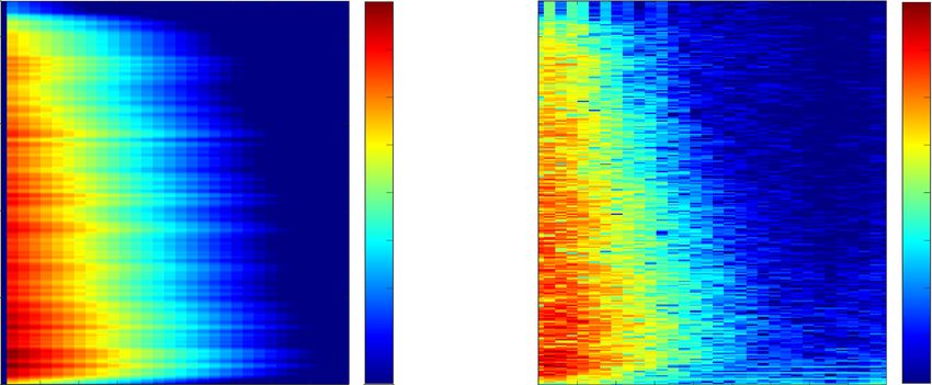
Gimm et al. EURASIP Journal on Audio, Speech, and Music Processing     (2021) 2021:21                                      Page 2 of 15

                                                                         reduced, the model-based approach will also affect the
                                                                         desired signal. However, due to the fact that speech is
                                                                         assumed to be short-time stationary and there is a delay
                                                                         in the processing and also in the path between loud-
                                                                         speaker and microphone, it is usually observed that the
                                                                         attenuation of the desired signal is small compared to the
                                                                         attenuation of the feedback signal. Hence, this method is
                                                                         able to increase the stability in closed-loop systems.
                                                                           In [8], we presented a method that makes use of the
                                                                         advantages of both described systems. Therefore, we
                                                                         introduced three ways to estimate the residual feedback
                                                                         PSD recursively, taking an adaptive filter into account. We
                                                                         also compared this with the model-based feedback sup-
                                                                         pression which was presented in [9]. In this work we made
                                                                         some improvements regarding the models. Furthermore,
                                                                         we show more implementation details. The objective eval-
                                                                         uation was improved by adjusting the features. Additional
 Fig. 1 Impulse response of a car cabin in the top graph, estimated      simulations were also performed to investigate the perfor-
 impulse response of an adaptive filter with length 1024 taps in the
                                                                         mance during room changes and the convergence of the
 middle graph, residual impulse response in the bottom graph
                                                                         adaptive filter in the presence of a postfilter. In addition,
                                                                         further acoustic paths were simulated.

impulse response hLM,i as well as the part ĥLM,i that an                1.1 Organization of this paper
adaptive filter has estimated. The bottom plot shows the                 The paper is organized as follows: after this introduction,
difference between the impulse response hLM,i and ĥLM,i .               previous research work is summarized in Section 2. After-
The estimation error h,i is the impulse response which                  wards the model-based feedback suppression approach is
causes the residual feedback in such a system.                           explained in Section 3. In Section 4, we show how we
   A different method to increase the stability gain in                  adapted the model-based approach to use it as a postfil-
electro-acoustic loops is to estimate the short-term power               ter. After that, we present different methods to derive the
spectral density (PSD) of the feedback by using the energy               required model parameters in Section 5. Finally, we show
envelopes of the room’s subband impulse responses.                       the evaluation procedure in Section 6 before a conclusion
These envelopes can be obtained by a priori or online                    is provided in Section 7.
measurements as well as simulations. With this informa-
tion, a model can be derived which is then used for a                    1.2 Notation
convolution with the loudspeaker subband power signal.                   Throughout this contribution the notation will follow
This results in an estimate of the feedback’s short-term                 some basic rules:
PSD. This estimate is then used within a so-called Wiener
filter (or a variant of it) to attenuate the feedback compo-               • Scalar quantities such as time-domain signals are
nents within the microphone signal. Except from online                       written in lowercase, non-bold letters such as s(n) for
measurements, the envelope is assumed to be constant.                        a signal at time index n.
However, it can be shown that the model-based methods                      • Short-term frequency-domain quantities are
are robust against room changes and that the envelopes                       described by upper case letters such as X(μ, k), with
vary only slightly over time. The main advantage of this                     k being the frame index and μ as frequency index.
method is that the model can be implemented recur-                         • Vectors are noted as bold letters, e.g., H(μ, k)
sively and, thus, very efficiently in terms of computational                 represents a vector containing filter coefficients in
complexity. There will not be any length limitations as                      subband μ at frame index k.
described when using adaptive finite impulse response                      • Smoothed signals are noted by over-lined letters such
(FIR) filters. However, there are disadvantages, too. The                    as x(n) and estimated signals are written as letters
main one lies in the derivation of the Wiener filter, which                  with a hat such as x̂(n).
assumes that both the desired and the undesired signals                    • All signals are represented in discrete time.
are orthogonal. In the presented application this is not
the case, since the feedback signal (undesired) is only a                2 Previous and related work
delayed and processed version of the local speech sig-                   Electro-acoustic feedback is a challenge in various tech-
nal (desired). This means that not only feedback will be                 nical systems. The most prominent ones are hearing aids,
Gimm et al. EURASIP Journal on Audio, Speech, and Music Processing (2021) 2021:21 Page 3 of 15 public address systems, and in-car communication sys- which is the end of a speech segment when there is still tems. Therefore, lots of research has been done in those some power in the loop due to the loop delay. domains in recent years. A comprehensive overview of In [9], the authors present a feedback suppression different approaches regarding feedback suppression can method based on well known speech dereverberation be found in [10]. In this work, we will focus on room techniques [27, 28]. Here, the feedback path is modeled modeling methods. with an statistical model. Based on this the feedback’s PSD To fully erase the feedback and, therefore, to allow arbi- is estimated. trary gains, the impulse response of the feedback path In [8], the model-based feedback suppression is tai- must be estimated by means of an adaptive filter. Early lored in a way that it can be used as a residual feedback approaches use a standard echo canceler to fulfill this suppression in combination with an adaptive feedback task [11–13]. Here, the impulse response is estimated e.g. canceler. Therefore, three adapted statistical models have with a normalized least mean square (NLMS) algorithm been proposed which can be used to model the feed- in the time domain. If the local signal and the excitation back path taking an adaptive filter into account. Model- signal are correlated, the problem is that adaptive filters based approaches have already been used in adaptive converge to a biased solution. This is strongly the case in echo cancelation systems [29, 30]. In [31], the authors closed-loop electro-acoustic systems [14]. also use a model-based approach as a postfilter for One solution to overcome this problem is to decorrelate adaptive echo cancelation. The idea is to use adaptive the signals. This can, for example, be realized by frequency approaches to model the residual echo power spectral shifting. It is shown in [15–17] that a slight frequency density. However, in all of these approaches the adap- shift within the frequency range of speech is sufficient to tive filter is assumed to work perfectly and only the improve the convergence of the adaptive filter. The sig- acoustic path, which is not covered by the filter is taken nals can also be decorrelated with linear prediction or into account. In AEC applications, this might be suf- pre-whitening [18]. In addition to the decorrelation of the ficient as reasonable steady-state performance can be signals, a special step-size control can further improve the reached. However, this is not the case in adaptive feedback convergence of the adaptive filter. In [1, 19], the decor- cancelation. relation methods frequency shift and pre-whitening are In the presented paper, the adapted models for residual compared and combined with a step-size control, based feedback suppression are further investigated and a more on a derivation of the so-called pseudo-optimal step size. detailed insight, as well as more simulations and results Another step-size control that is able to improve the are given. convergence of the adaptive filter without the need of any decorrelation method is described in [20, 21]. Here, 3 Model-based feedback suppression the reverberation of the system is exploited to adapt the In [9] it was shown that room dereverberation techniques filter, since signals are not correlated during reverbera- as they were introduced in e.g. [27, 28] can be used to tion. With this step-size control, both stability and speed increase the stability of closed electro-acoustic loops as we of convergence can be improved also for high system face them in ICC systems. In this section, the model-based gains. feedback suppression will be described before adapting it One drawback of the feedback cancelation approaches for a system with feedback cancelation. We will start with is that the adaptive filter must cover the relevant length linear, time-invariant systems with coefficient index i. Of of the room’s impulse response. Otherwise, residual feed- course, we can assume here only short-term stationar- back is audible and may even cause the system to become ity. Therefore, we will introduce time-variance (by adding instable. Since long filters increase the computational also a frame index k) after this generic view on the entire complexity as well as the convergence time, short filter system. lengths are often preferred. A simple example of a time-domain system operating in In the field of acoustic echo cancelation (AEC), postfil- a closed electro-acoustic loop can be seen in Fig. 2. ters based on frequency-domain Wiener filters are com- The signal y(n) is the microphone signal at time index monly used [22–25]. The idea is that the residual echo is n and g is a Wiener filter with coefficients based on nothing but the undisturbed error signal which is the sig- the estimated feedback which is used to suppress the nal after the subtraction of the AEC took place assuming recorded feedback that is present in y(n). hSE is the the absence of any local speech and noise signals. A very impulse response that belongs to the system of the indi- similar approach was already used for residual feedback vidual application, where SE stands for signal enhance- suppression [13]. The downside of this technique is that ment. It differs with the individual application and may the PSD estimation should only be done in remote single include noise suppression in case of an ICC system or an talk conditions [26]. Such a situation does not exist in case equalization filter in case of a public address (PA) system. of closed-loop systems. There is however one exception After the signal enhancement stage, x(n) is played back
Gimm et al. EURASIP Journal on Audio, Speech, and Music Processing           (2021) 2021:21                                        Page 4 of 15

                                                                                 To make this method more robust against small varia-
                                                                               tion in hLM and to get the ability to save computational
                                                                               complexity we define a model of hLM based on its so-
                                                                               called reverberation time T60 and some other parameters,
                                                                               which will be explained next.
                                                                                 This finally results in an exponentially decaying model
                                                                               of the power envelope of the subband version of H LM (μ)

                                                                                   H LM,mod,A (μ, k)2                              (8)

                                                                                           0,                       for k < P(μ),
                                                                                       =                                             (9)
                                                                                           A(μ) e  −γ (μ)(k−P(μ)) , for k ≥ P(μ),
 Fig. 2 Structure of a single-channel, closed-loop system with
 feedback suppression, which is first of all assumed to be time invariant
                                                                               where μ is the discrete subband index, k is the frame index
                                                                               and A(μ) are coupling factors that describe the coupling
                                                                               properties of the acoustic path. P(μ) is the delay of the
using a loudspeaker resulting in a feedback r(n). The latter                   acoustic path in frames and
is obtained by a convolution of x(n) with the room impulse
                                                                                               2 · 3 ln(10)L
response hLM . As mentioned above, the room impulse                                γ (μ) =                                                (10)
response is assumed to be constant for now. Thus, the                                            T60 (μ) fS
time index n can be dropped and we obtain the feedback                         describes the decay behavior, where L denotes the
signal as                                                                      frameshift in samples. Using Eq. (8) the estimated short-
             ∞
                                                                              time PSD of the current feedback Ŝrr,A (μ, k) can be cal-
    r(n) =         x(n − i) hLM,i .                                    (1)     culated as the convolution of the short-time PSD of the
             i=0                                                               loudspeaker signal Ŝxx (μ, k) with the magnitude square of
r(n) is recorded again by the microphone together with                         the modeled subband impulse response
additional background noise b(n) and local speech s(n),                            Ŝrr,A (μ, k)
yielding the microphone signal                                                                 ∞

    y(n) = s(n) + b(n) + r(n).                                         (2)                 =     Ŝxx (μ, k − i) A(μ) e−γ (μ)(i−P(μ))
                                                                                              i=P(μ)
  The transfer function of the entire electro-acoustic loop
                                                                                          = A(μ)Ŝxx (μ, k − P(μ))
can be described as follows:
                                                                                           + e−γ (μ) Ŝrr,A (μ, k − 1).               (11)
        j            HSE ej G ej
   HL e       =                          .         (3)                      On the top left of Fig. 3, the energy envelope of the
                1 − HSE ej G ej HLM ej
                                                                               modeled subband impulse response for a single subband
  Here,  = 2πf /fS ∈[ 0, 2π) is the frequency f normal-                       is depicted. This can now be used for a subband version
ized with respect to the sampling frequency fS . Further-
more,                                                                                                        Ŝrr,X (μ, k)
                                                                                   GX (μ, k) = max 0, 1 −                           (12)
                                                                                                      Ŝyy (μ, k)
    C ej = HSE ej G ej HLM ej                     (4)
is the so-called open-loop gain. For stability reasons                         of Eq. (7), with X indicating the individual model type, e.g.,
       j                                                                  X=A.
     C e  < 1 ∀                                                     (5)
and
                                                                               4 Model-based feedback suppression as postfilter
                                                                             Due to stability reasons, FIR filters are commonly used in
    ∠C ej  = η2π ∀, η ∈ Z+
                            0                                          (6)     adaptive filter applications like echo- or feedback cance-
                                                                               lation. If this kind of method is used in a closed electro-
should hold. G(ej ) can be used to fulfill this condition.
                                                                               acoustic loop system, it is capable of subtracting parts
One possibility would be to choose the transfer function
                                                                               of the feedback signal r(n) from the microphone signal
based on the estimated feedback
                                                                             y(n) depending on how good it is adapted to the true
      j        Ŝrr ej                                                     room impulse response. However, there are some limita-
   G e      =1−        .                              (7)
                  Ŝyy ej                                                     tions in the steady-state performance. One of them is that
                                                                               there will always be a residual system mismatch which is
  Therefore, an estimate of the feedback PSD Ŝrr (ej ) is                    caused by non-optimal control or estimation errors, even
required, which can be derived from Eq. (1).                                   if robust adaptive control schemes are used. If an efficient
Gimm et al. EURASIP Journal on Audio, Speech, and Music Processing (2021) 2021:21 Page 5 of 15
Fig. 3 Overview of the four different models
implementation in the subband domain is chosen, the per- Because of its recursive nature, the model will also cover
formance is also limited due to aliasing effects caused by rooms with a long reverberation time without signifi-
the filter banks. The other limitation is due to the part of cant impact on the complexity. However, it has to be
the true room impulse response which cannot be covered adapted with respect to the presence of the adaptive fil-
by the adaptive filter. This happens because the FIR fil- ter. Therefore, the effective impulse response, which is a
ter needs to be implemented with a fixed length, which is combination of the true impulse response and the one
often restricted by computational complexity. estimated by the adaptive filter, needs to be computed to
Here, a postfilter is usually used to suppress the parts derive a new model. The effective impulse response can
of the feedback which remain after a feedback cancelation be derived using the signal e(n) from Fig. 4. For this signal
approach as it is depicted in Fig. 4. holds:
The idea is to use the method proposed in the previ- ∞
ous section and adapt it, so it can be used as a postfilter. e(n) = s(n) + b(n) + x(n − i) hLM,i (n) − r̂(n)
i=0
∞
= s(n) + b(n) + x(n − i) hLM,i (n) − xT
m (n) ĥLM (n)
i=0
∞
= s(n) + b(n) + x(n − i) hLM,Res,i (n).
i=0
(13)
Here,
T
ĥLM (n) = ĥLM,0 (n), ĥLM,1 (n), · · · , ĥLM,m-1 (n) (14)
is a vector containing the adaptive filter coefficients and
Fig. 4 Structure of a single-channel system in a closed loop with
feedback canceler and residual feedback suppression
xm (n) = [x(n), x(n − 1), · · · , x(n − m + 1)]T (15)Gimm et al. EURASIP Journal on Audio, Speech, and Music Processing (2021) 2021:21 Page 6 of 15
contains the m latest samples of x(n), where m is the num- feedback Ŝrr,B (μ, k) can be obtained by convolving this
ber of filter coefficients in the adaptive filter. With this the modeled subband impulse response with the PSD of the
effective impulse response can be derived as: loudspeaker signal yielding a solution consisting of two
parts:
hLM,Res,i (n)
Ŝrr,Res,B (μ, k)
hLM,i (n) − ĥLM,i (n), for 0 ≤ i < m,
=
M−1
hLM,i (n), else, = Ŝxx (μ, k − i) M H (μ, k)2
i=0
hLM,,i (n), for 0 ≤ i < m,
= (16) ∞
hLM,i (n), else. + Ŝxx (μ, k − i) A(μ) e−γ (μ)(i−P(μ))
i=M
As one may expect, knowledge about the actual sys-
tem mismatch for each subband is necessary as it has an
M−1
= Ŝxx (μ, k − i) M H (μ, k)2
influence on the amount of residual feedback. Another
i=0
difference compared to model A is that there is a direct ∞
connection from the loudspeaker signal to the error signal + Ŝxx (μ, k − i − M) A(μ) e−γ (μ)(i−P(μ)+M)
now which is caused by the misalignment in the adaptive i=0
filter.
= Ŝxx,rec (μ, k) M H (μ, k)2 + Ŝmm (μ, k). (20)
However, this is unknown and has to be estimated.
Furthermore, assumptions about the shape of the system Each of these two parts can be calculated recursively,
misalignment over filter taps has to be made. leading to a very low computational complexity:
During the time when adaptive filters were being stud- Ŝxx,rec (μ, k) = Ŝxx,rec (μ, k − 1)
ied very extensively—decades ago—two different ideas of
the progress of the filter coefficients during an adaptation +Ŝxx (μ, k) − Ŝxx (μ, k − M) (21)
period co-existed—and still do so today. Ŝmm (μ, k) = e−γ (μ) Ŝmm (μ, k − 1)
4.1 Model B
+Ŝxx (μ, k−M) A(μ) e−γ (μ)(M−P(μ)) .
One idea is that adaptive algorithms spread the error (22)
more or less equally over all coefficients. As a conse- In the top right of Fig. 3, the energy envelope of the
quence, the system mismatch vector can be modeled as subband-impulse response for a single subband of model
a white process with zero mean and a time-variant, but B compared to model A (introduced in the previous
lag-independent variance. Our investigations showed that section) can be seen.
this seems to be correct if the filter is well converged. So
the first approach is to model a constant system mismatch 4.2 Model C
for all filter taps, yielding a power envelope of the residual The second idea is that the system mismatch of the indi-
subband impulse response: vidual coefficients is more or less proportional to the
magnitude of the room impulse response of the system
HLM,mod,B (μ, k)2
that should be identified. This behavior is also observ-
M H (μ, k)2 , for 0 ≤ k ≤ M − 1, able, but mainly at the beginning of adaptation processes
= (17)
A(μ) e −γ (μ)(k−P(μ)) , for M ≤ k. or—in general—whenever the filter is not well adapted.
Since feedback cancelation approaches for ICC systems
In this work, this approach is named model B. M is face generally hard conditions e.g. permanent double-talk
the filter length in frames. In case of subband processing, and high background noise levels, this model would be an
H (k) is a vector containing the system mismatch vector option here.
in every subband. To model this we assume the first interval for the direct
H (μ, k)2 = H(μ, k) − Ĥ(μ, k)2 (18) part of the residual impulse response to be zero. This is
usually the case only when the adaptive filter is initialized.
M−1
After some iterations the coefficients will differ from zero.
= |H(μ, k − j) − Ĥ(μ, k − j)|2 (19)
However, the system mismatch in this interval will always
j=0
stay small compared to the interval between the largest
is a vector containing the norms of the system mis- coupling and the rest of the adaptive filter. Here, the sys-
match vectors. This is often estimated within adaptive tem mismatch is modeled as exponentially decaying with
control schemes. An overview about several estimation the same T60 as it is used in all other approaches. Fur-
procedures can be found in [32]. The estimated residual thermore, we introduce Q(μ) which is the power of theGimm et al. EURASIP Journal on Audio, Speech, and Music Processing (2021) 2021:21 Page 7 of 15
maximum value in the system mismatch vector. This leads To follow this approach, the time-domain impulse
to the following power envelope of the model response has to be transformed into the subband domain
N−1
HLM,mod,C (μ, k)2 μκ
⎧ HLM (μ, k) = hana,κ hLM,kL+κ e−j2π N , (27)
⎪
⎨ 0, for k < P(μ), κ=0
= Q(μ, k) e −γ (μ)(k−P(μ)) , for P(μ) ≤ k < M, (23) where N is the window length and, thus, the length of the
⎪
⎩
A(μ) e −γ (μ)(k−P(μ)) , for M ≤ k. DFT, and hana is the window function used in the filter
bank. The absolute value of the subband impulse response
Using this model, the PSD of the residual feedback can is smoothed along the frequency axis in both positive
be calculated as follows: (Eq. (28)) and negative (Eq. (29)) direction for every frame
with the smoothing constant ζ :
Ŝrr,Res,C (μ, k)
M−1 H̃ LM (μ, k)
= Ŝxx (μ, k − i) Q(μ) e−γ (μ) i−P(μ)
=(1 − ζ ) H̃ LM (μ − 1, k) + ζ |H LM (μ, k)| (28)
i=P(μ)
∞ H̄ LM (μ, k)
+ Ŝxx (μ, k − i) A(μ) e−γ (μ) i−P(μ)
(24) =(1 − ζ ) H̄ LM (μ + 1, k) + ζ H̃ LM (μ, k). (29)
i=M
This way, a zero-phase low-pass filter is realized to
reduce the variance along the frequency axis. As a first
= e−γ (μ) Ŝrr,Res,C (μ, k − 1) step, the delay can be determined for each subband by
+ Ŝxx μ, k − P(μ) Q(μ, k) finding the index of the first maximum value of the
smoothed magnitude subband impulse response in each
+ Ŝxx (μ, k−M) A(μ)−Q(μ) e−γ (μ) M−P(μ) . subband
(25) P(μ) = argmax H̄ LM (μ, k) λk , (30)
k∈[0,1,··· ,LLM −1]
4.3 Model D with LLM representing the considered length of the
The drawback of the two proposed models is that the impulse response in frames and λk representing an expo-
performance will depend on how accurate the estimation nentially decaying series with λ ∈ (0, 1), which can be
of the system distance is. An easier method compared used to avoid choosing late constructive interferences as
to models B and C is to assume that the adaptive filter maxima.
operates perfectly well and there is consequently only the Next, a vector of length MLM is defined for every
length limitation which has to be covered by the postfil- subband. It contains the logarithmic impulse responses,
ter. This would be advantageous, but it is not very realistic starting at the delay which was found before:
in practical approaches. Models B and C are better in this
regard. In this case, H (μ, k)2 can be set to zero and the h̆LM (μ) = ln H̄LM (μ, P(μ)) , · · · ,
estimated PSD of the feedback signal simplifies to T
ln H̄LM (μ, MLM + P(μ)) . (31)
Ŝrr,Res,D (μ, k)
This can be modeled linearly for each subband
= e−γ (μ)(M−P(μ)) A(μ) Ŝxx (μ, k − M)
+e−γ (μ) Ŝrr,Res,D (μ, k − 1), (26) h̆LM (μ, k ) = Ã(μ) + γ̃ (μ)k (32)
k ∈ {0, 1, · · · , MLM − P(μ) − 1} .
which corresponds to Ŝmm (μ, k) in Eq. (22).
Written in matrix notation, the logarithmic subband
5 Model parameters impulse responses can be combined to
To use the proposed model-based approach, a priori h̆LM = , (33)
knowledge about the room is needed. In this work, the
room is assumed to be power stationary, meaning that the where is the observation matrix and represents the
power envelope of the room impulse response does not parameter vector
vary much over time. Depending on the particular control ⎡ ⎤
0 1
mechanism used for the adaptive filter, a correction of the ⎢1 1⎥
⎢ ⎥ γ̃ (μ)
model parameters based on the adaptive filter is also pos- = ⎢. .. ⎥ , = . (34)
sible. The parameters can be extracted using a measured ⎣ .. . ⎦ Ã(μ)
impulse response like it was proposed in [33]. MLM − P(μ) − 1 1Gimm et al. EURASIP Journal on Audio, Speech, and Music Processing (2021) 2021:21 Page 8 of 15
To find the unknown parameters in , Eq. (33) can be example shown in Fig. 5. Using this value the decay instant
modified according to can be derived:
−1 2 · 3 ln(10) L
= T T h̆LM , (35) γ (μ) ≈ γ = ∀μ. (40)
T60 fS
−1 The remaining parameters which need to be estimated
with T T = † being the pseudo inverse of .
are the coupling factors. These are the absolute squared
The last step is to convert the logarithmic values to linear values of the maximum of the subband impulse response,
values which can be found at frame index k = P according
γ (μ) = eγ̃ (μ) , (36) to Eq.(30). Therefore, the smoothed version of Eq. (29)
should be used to reduce the variance along the frequency
A(μ) = eÃ(μ) . (37) axis to yield
A simplification, which we also used for our simula- 2
A(μ) = H̄ LM (μ, P) . (41)
tions, would be to assume the model parameters except
the coupling factors to be identical for all frequencies. In In Fig. 6, a time-frequency analysis of the measured
this case, the delay and the decay constants can be com- impulse response and the corresponding model can be
puted directly from the energy decay curve (EDC) defined seen.
as
−1
NLM 6 Results and discussion
|hLM,i |2 The proposed schemes were tested in an ICC application.
i =i
EDC(i) = . (38) For this, an impulse response measured in a van was used.
−1
NLM
It is the same one as shown in Fig. 5. The complete setup
|hLM,i |2
i =0 is shown in Fig. 7.
The EDC describes the remaining energy in the system For our simulation we used clean speech signals from
at time instance i normalized to 0 dB. An example of an different male and female speakers sampled at 44.1 kHz.
EDC measured in a car cabin can be seen in Fig. 5. The The DFT order was set to N = 512 and we used a
delay TD is the time instant where the EDC begins to drop. frameshift of L = 256. The NLMS-based adaptive filter
Using this value, the delay in frames can be derived as Ĥ(μ, k) =Ĥ(μ, k − 1)
fS E∗ (μ, k − 1)X(μ, k − 1)
P(μ) ≈ P = TD · ∀μ, (39) +α (42)
L X(μ, k − 1)2
with ... denoting rounding towards the next smaller inte- with a fixed step-size α and E(μ, k) and X(μ, k) being the
ger. The reverberation time T60 is the time instant when error signal or the excitation signal vector, respectively,
the energy that remains in the tail of the room impulse was adapted until a specific system distance for all sub-
response reaches − 60 dB. Often, this cannot be found in bands was obtained. Afterwards the adaption was stopped
the EDC, because there is measurement noise dominating by setting α to zero. As the system distance for this par-
when using a measured impulse response. In this case, the ticular simulation was known, we used this value also as
EDC has to be extrapolated linearly, as it was done in the a parameter in model B and C to avoid the influence of
Fig. 5 Energy decay curve and coupling factors of an impulse response measured in a car cabinGimm et al. EURASIP Journal on Audio, Speech, and Music Processing (2021) 2021:21 Page 9 of 15
Fig. 6 Measured and modeled time-frequency representation of the energy envelope of hLM
estimation errors. M was set to four frames, correspond- with
ing to a filter length of 46.4 ms. Afterwards the step-size
Sss (μ, k) r (μ, k)
was set to zero for the simulation. This was done since P̃r (μ, k) = 10 log10
the models would affect the convergence behavior of the Sss (μ, k) r (μ, k) GX2 (μ, k)
adaptive filter, so the results would also be affected. The
1
aim of the postfilter is to reduce the residual feedback in = 10 log10 , (46)
GX (μ, k)
2
the microphone signal as much as possible without affect- r (μ,k) =0
ing the desired speech signal. To prove this, the ratio of the where NFrames is the total number of processed frames
mean logarithmic speech power and the mean weighted in this simulation and μz ∈[ μStart , μStart+1 , · · · , μStop ]
logarithmic speech power was calculated as are the investigated subbands representing frequencies
between about 90 Hz and 8000 Hz, where most of the
μStop
−1
NFrames speech power is located. Sss (μ, k) is the short-term power
P̃s (μ, k)
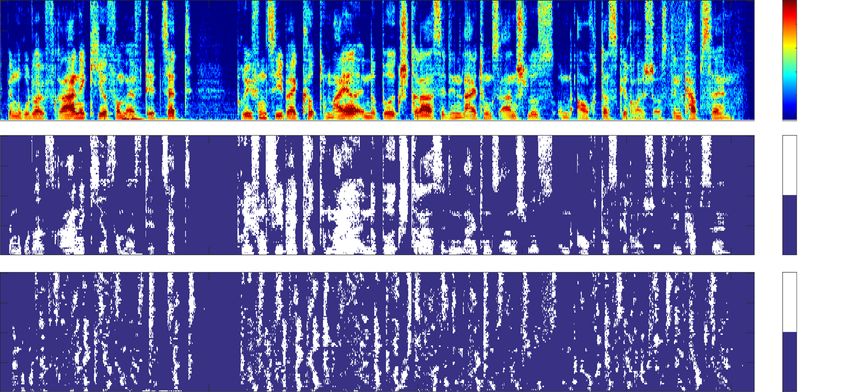
k=0 μ=μStart spectrum of the input frame of the clean speech signal.
Ps = (43) s (μ, k) is a binary mask based on a subband voice activ-
−1 μ
NFrames Stop
s (μ, k) ity detection which is one for subbands where voice is
k=0 μ=μStart detected and zero for those without voice. r (μ, k) is the
equivalent for the reverberation signal with the additional
with condition that all time-frequency bins where s (μ, k) = 1
are set to zero. An example of the described masks can be
Sss (μ, k) s (μ, k) seen in Fig. 8, where the speech signal of the investigated
P̃s (μ, k) = 10 log10
Sss (μ, k) s (μ, k) GX2 (μ, k)
1
= 10 log10 2 (μ, k)
. (44)
GX
s (μ,k) =0
The same can be done for the reverberation parts of the
signal
μStop
−1
NFrames
P̃r (μ, k)
k=0 μ=μStart
Pr = (45)
−1 μ
NFrames Stop
r (μ, k) Fig. 7 Structure of a single-channel system used for the simulation
k=0 μ=μStartGimm et al. EURASIP Journal on Audio, Speech, and Music Processing (2021) 2021:21 Page 10 of 15
Fig. 8 Spectrogram of the speech signal at the top, speech active mask in the middle and reverberation active mask at the bottom
subbands is at the top, the mask for the clean speech is in
the middle, and the mask for the reverberation is at the Table 1 Simulation results for the four different models at
bottom. Using these masks, the impairment is only evalu- different system distances
ated where the respective signals are present. The reason System-distance/dB Model Ps Pr (Pr − Ps ) STOI
for using this method is that we wanted to observe the /dB /dB /dB
ratio between speech impairment and feedback suppres-
− 40 A 10.72 18.22 7.50 0.86
sion as well as both quantities alone. This is important
because a large speech impairment could lead to audible B 5.29 15.24 9.95 0.94
artifacts. More established methods like segmental SNR C 5.24 15.24 10.00 0.94
would only show the feedback reduction, which is not D 5.24 15.25 10.01 0.94
sufficient for our purpose. - 0 0 0 0.99
Furthermore, we used a short-time objective intelli-
gibility (STOI) measure, which was proposed in [34]. − 30 A 10.72 18.46 7.74 0.86
This measurement shows good performance in evaluating B 5.64 15.67 10.03 0.94
degradation caused by time-frequency based algorithms C 5.25 15.27 10.02 0.94
e.g. noise reduction. As a reference signal we used the D 5.24 15.27 10.03 0.94
clean speech s(n). The loudspeaker signal x(n) was the - 0 0 0 0.99
signal to be evaluated.
In Table 1, the simulation results for different system − 20 A 10.69 18.03 7.34 0.86
distances are shown. Ps is the unwanted impairment of the B 7.97 16.66 8.69 0.91
clean speech signal, Pr is the equivalent for the reverbera- C 5.35 14.26 8.91 0.94
tion signal. Pr − Ps is the distance between both. Since one D 5.25 13.96 8.71 0.94
impairment is wanted and the other one is not, it describes
- 0 0 0 0.99
the attenuation of the unwanted signal. Consequently Ps
has to be treated as an offset and needs to be compensated. − 10 A 10.77 16.98 6.21 0.84
When the system distance is at − 40 dB, the results in B 13.68 18.34 4.66 0.77
terms of the different approaches (B–D) for Pr − Ps as well C 6.19 13.05 6.86 0.91
as STOI are similar. However, it can also be seen that the D 5.14 11.73 6.59 0.92
impairment of the clean speech is significantly higher in
- 0 0 0 0.95
case of model A, which is the original unadapted model.Gimm et al. EURASIP Journal on Audio, Speech, and Music Processing (2021) 2021:21 Page 11 of 15
Model B, which is assumed to be correct for this simula- T60 = 80.3 ms compared to the original 119.9 ms as well
tion because the filter is well adapted and has a constant as different coupling factors, which can be seen in Fig. 9.
system mismatch, is very similar to models C and D with The results (see Table 2) show that both STOI and (Pr −
respect to Ps and Pr . This happens due to the fact that in Ps ) are only slightly worse than before, but still very good.
case of a small system distance models (B–D) are nearly In order to have a more robust evaluation, we simu-
the same. When the system distance is increased, the lated a second acoustic path. This time it is one that was
impairment of the clean speech caused by models A and recorded in a lecture hall and has a significantly longer
D are nearly constant whereas it increases in case of mod- decay time T60 of 777.8 ms. The delay TD is 18.7 ms.
els B and C. This is exactly what one would expect because The results can be seen in Table 3. The higher reverber-
of the short-time stationary nature of speech leading to a ation time results in a slightly higher influence on the
large correlation when reducing the lag between an input desired signal than in the simulation before. However, a
frame and the models response. The system distance is clear attenuation of the feedback can still be seen. The pre-
used as a weight. By increasing it while decreasing the viously discussed effects of the different models apply here
response time the correlation between the wanted and the without restriction.
unwanted signal increases. In order to evaluate the subjective impairment of the
In case of model B, there is an immediate response to desired signal we conducted a listening test with 26
an input signal. Model C also produces a response in the untrained participants aged between 21 and 46 years.
region of early feedback, resulting in a higher value of Ps We used the same setup as shown before with a system
when increasing the system distance. However, Pr − Ps distance of −30 dB.
is slightly better than in case of all other models. The Overall the procedure was a degradation category rat-
best compromise regarding the impairment of the clean ing (DCR) according to ITU-T Rec. P.800 [35], which
speech is reached with models C and D. Evaluating with was modified for our purpose. We always played the
STOI shows similar results. It can be seen that the results unprocessed clean speech signal as reference and then the
improve when the system distance decreases. For large simulated versions with either one of the models (A–D) or
system distances the scores are low even if there is no the cancelation only (–) in random order. We used three
postfilter applied (-). This is due to the existing feedback female and two male speakers saying German sentences
in the processed signal. For a system distance of −10 dB according to ITU-T Rec. P.501 [36]. In sum, every partici-
it can also be seen that the score of model D is slightly pant had to rate 25 signals. One of the female speakers was
higher, although Pr − Ps of model C is slightly larger. used for a trial run which we did not take into account to
This is due to the fact that model D causes less speech give the participants the opportunity to get used to the test
impairment in this particular setup. Furthermore, a rela- procedure. The signals are provided on a web page [37].
tion between STOI and Ps can be observed. A large value The rating was defined as following:
for Ps leads to a low STOI rating, which is due to the
fact that STOI evaluates the degradation of the speech • 5. Excellent – Speech sounds like the unprocessed
signal, which is mainly influenced by Ps . The best results signal
in terms of STOI are reached when there is no postfil-
ter at all. However, this does not mean that it makes no
sense to use a postfilter at all, because one of its main
purpose is to increase stability while saving computing
power.
The impulse responses used for the model-based
approach were measured under certain conditions. For
example, this could be an empty vehicle at a certain
temperature. In reality, however, these are subject to per-
manent fluctuations due to room changes. For example,
a car could be fully loaded and fully occupied or empty.
In addition, objects directly in front of sound sources or
microphones could cause large attenuation.
Even changes in the distance between loudspeaker and
microphone are conceivable. In the following, we will
investigate such a situation where the model parame-
ters are determined based on an impulse response of an
empty van, but in fact there is a fully occupied interior. Fig. 9 Coupling factors of the empty car used as model parameters
for simulation and true coupling factors of the fully loaded car
This variation of the acoustic path results in a reducedGimm et al. EURASIP Journal on Audio, Speech, and Music Processing (2021) 2021:21 Page 12 of 15
Table 2 Simulation results for the four different models at Table 3 Simulation results for the four different models at
different system distances with incorrect system parameters after different system distances with impulse response of a lecture
a room change room
System-distance/dB Model Ps Pr (Pr − Ps ) STOI System-distance/dB Model Ps Pr (Pr − Ps ) STOI
/dB /dB /dB /dB /dB /dB
− 40 A 10.72 18.08 7.36 0.86 − 40 A 12.94 19.33 6.39 0.80
B 5.29 14.26 8.97 0.94 B 6.84 17.24 10.40 0.90
C 5.28 14.22 8.94 0.94 C 6.84 17.24 10.40 0.90
D 5.28 14.23 8.95 0.94 D 6.84 17.24 10.40 0.90
- 0 0 0 1.00 - 0 0 0 0.99
− 30 A 10.72 17.90 7.18 0.86 − 30 A 12.94 19.25 6.31 0.80
B 5.41 13.90 8.49 0.94 B 6.90 17.25 10.35 0.90
C 5.28 13.75 8.47 0.94 C 6.84 17.24 10.40 0.90
D 5.28 13.73 8.45 0.94 D 6.84 17.24 10.40 0.90
- 0 0 0 1.00 - 0 0 0 0.99
− 20 A 10.74 17.14 6.40 0.86 − 20 A 12.94 18.82 5.88 0.80
B 6.60 14.00 7.40 0.93 B 7.41 17.07 9.66 0.90
C 5.30 12.42 7.12 0.94 C 6.88 16.59 9.71 0.90
D 5.26 12.29 7.03 0.94 D 6.87 16.58 9.71 0.90
- 0 0 0 1.00 - 0 0 0 0.99
− 10 A 10.73 16.41 5.68 0.86 − 10 A 12.94 17.72 4.78 0.80
B 11.47 16.60 5.19 0.83 B 10.50 17.39 6.89 0.87
C 5.63 11.24 5.61 0.93 C 6.96 14.80 7.84 0.89
D 5.20 10.41 5.21 0.93 D 6.92 14.76 7.84 0.89
- 0 0 0 0.99 - 0 0 0 0.98
• 4. Good – Speech is slightly impaired, but sounds The results in Table 4 are consistent with the objective
natural results, with the exception of STOI. In the hearing test, the
• 3. Fair – Speech is impaired, but the artifacts are not subjects rated a larger feedback as disturbing as a strong
disturbing degradation of the speech signal. In contrast, the results
• 2. Poor – Speech quality degrades, interfering according to STOI must be interpreted in such a way that a
artifacts are clearly audible stronger feedback has less influence than the degradation
• 1. Bad – Speech is heavily impaired of speech.
In a next step, we want to evaluate the model influence
The results in terms of a mean opinion score (MOS) can on the convergence behavior of an adaptive filter. For this,
be seen in Fig. 10. we used an NLMS-based adaptive filter based on pseudo-
The unadapted model and the version without any post- optimal step-size
filter were rated with a mean opinion score below 2.5. This
shows that artifacts caused by the postfilter are as bad as E |Eu (μ, k)|2
α opt (μ, k) ≈ (47)
the residual feedback when there is no postfilter at all. All E |E(μ, k)|2
of the adapted models are rated with a MOS between 3.2
and 3.6 which means that the impairment is less compared according to [26], where the expected value E{·} was
to the unadapted model. Here model C shows the best approximated by first order IIR smoothing. The so-called
results compared to models B and D. However, a Tukey undisturbed error Eu (μ, k), which is the error signal
honest significant difference (HSD) test with α = 0.05 as E(μ, k) without local signals, must be estimated as well.
suggested in [35] shows that there is no significant dif- For this, it is replaced by
ference between models B, C, and D as well as between
Eu (μ, k) = E(μ, k) − S(μ, k) − B(μ, k) (48)
model A and no postfilter at all. However, the approaches
can be grouped in model (B, C, and D) and (A and −). = HH
(μ, k)X(μ, k), (49)Gimm et al. EURASIP Journal on Audio, Speech, and Music Processing (2021) 2021:21 Page 13 of 15
|E(μ, k)|2 − Ŝbb (μ, k)
βx2 (μ, k) = βLEM
2
(μ, k) · (51)
|Y (μ, k)|2 − Ŝbb (μ, k)
2
= βLEM (μ, k) · βy2 (μ, k), (52)
2 (μ, k) being a pre-measured quantity based on
with βLEM
A(μ) and βy2 (μ, k) being the smoothed power ratio of the
microphone and the error signal.
For the simulation, we used speech signals recorded in
a car at 100 km/h. Now we replaced the fixed values of
||H (μ, k)||2 with its estimate which we get from the step-
size control βx2 (μ, k). Q(μ, k) in model C was replaced
with MA(μ)βx2 (μ, k). The loop gain initially was at 5 dB
and was increasd with 0.8 dB/second until it reached the
final value of 28 dB. The results in terms of the system
distance over time with the same adaptive filter and the
Fig. 10 Results (mean opinion score and variance) of subjective different models for the postfilter are shown in Fig. 11.
evaluation for the adaptive filter only (−), the “standard” model (A), It can be seen that the best performance is reached when
the model with const. system mismatch (B), the model with an
exponentially decaying shape of the system mismatch (C), and the
there is no postfilter at all. This is due to the fact that the
model based on perfect adaptive filter (D) achievable system distance at a fixed step-size depends
only on the power ratio between feedback signal and local
signal [26]. Even with an adaptive step-size control, as in
this case, it does not always work well enough to compen-
sate for this. As mentioned before, this is mainly due to
with H (μ, k) being still not known. First, we replace it
Ps . This value attenuates the desired signal, which reduces
with an estimate yielding
the power of the loudspeaker signal by the same amount.
To adjust the achievable filter performance, the filtered
2
¯ signal must be amplified by the value Ps , which is shown
Êu (μ, k) = |X̄(μ, k)|2 · βx2 (μ, k). (50) in Fig. 12.
Here, we adjusted the gain by an offset of 5 dB in case of
models C and D and 10 dB in case of model A. For these
In acoustic echo cancelation, βx2 (μ, k) could be esti- three models this nearly matches the individual values of
mated by minimum tracking the power of the noise- Ps . However, this did not work for model B, where we had
reduced error signal, which is then divided by the to add 17 dB to the loop gain. The difference is that Ps of
smoothed power of X(μ, k). However, this is not possible models A,C, and D has only a small or no dependency on
in feedback cancelation due to the permanent presence of
local speech. Here, an approach [38] is to split βx2 (μ, k)
into
Table 4 Results of Tukey’s HSD test with α = 0.05
Model 1 Model 2 Mean Adjusted Reject
difference p value
(−) A 0.2596 0.1635 False
(−) B 1.0481 0.001 True
(−) C 1.3077 0.001 True
(−) D 1.125 0.001 True
A B 0.7885 0.001 True
A C 1.0481 0.001 True
A D 0.8654 0.001 True
B C 0.2596 0.1635 False
B D 0.0769 0.9 False Fig. 11 System distance of adaptive filter over time with different
C D − 0.1827 0.5075 False modelsGimm et al. EURASIP Journal on Audio, Speech, and Music Processing (2021) 2021:21 Page 14 of 15
Acknowledgements
The authors would like to thank all participants of the hearing test.
Authors’ contributions
MG and PB have conducted the research and analyzed the data. MG, PB, and
GS authored the paper. All authors read and approved the final manuscript.
Funding
Open Access funding enabled and organized by Projekt DEAL.
Availability of data and materials
The sample files which we used for the subjective evaluation can be found
online [37].
Declarations
Competing interests
The authors declare that they have no competing interests.
Fig. 12 System distance of adaptive filter over time with different Author details
1 Digital Signal Processing and System Theory, Kiel University, Kaiserstr. 2,
models with gain adjustment
24143 Kiel, Germany. 2 Cerence, Soeflinger Strasse 100, 89077 Ulm, Germany.
Received: 18 May 2020 Accepted: 6 April 2021
the system distance, whereas it increases with decreasing References
system difference in case of model B. 1. F. Strasser, H. Puder, Adaptive feedback cancellation for realistic hearing
aid applications. IEEE/ACM Trans. Audio Speech Lang. Process. 23(12),
2322–2333 (2015). https://doi.org/10.1109/TASLP.2015.2479038
7 Conclusion 2. A. Spriet, S. Doclo, M. Moonen, J. Wouters, Feedback Control in Hearing Aids.
In this work, we investigated existing and proposed (J. Benesty, M. M. Sondhi, Y. A. Huang, eds.) (Springer, Berlin, Heidelberg,
2008), pp. 979–1000. https://doi.org/10.1007/978-3-540-49127-9_48
slightly extended postfilter schemes which are capable 3. B. C. Bispo, D. Freitas, in E-Business and Telecommunications. ICETE 2014.
of suppressing residual feedback in closed-loop systems Communications in Computer and Information Science, ed. by M. Obaidat,
where adaptive feedback cancelers are used. We showed A. Holzinger, and J. Filipe. Performance evaluation of acoustic feedback
cancellation methods in single-microphone and multiple-loudspeakers
that there are different ways to adapt the reverberation public address systems, vol. 554 (Springer, Cham, 2015). https://doi.org/
model with respect to the feedback canceler. We were 10.1007/978-3-319-25915-4_25
able to show by means of subjective and objective evalu- 4. G. Rombouts, T. van Waterschoot, K. Struyve, M. Moonen, Acoustic
ation that all of our adapted models provide a better per- feedback cancellation for long acoustic paths using a nonstationary
source model. IEEE Trans. Signal Process. 54(9), 3426–3434 (2006). https://
formance then using the standard reverberation model doi.org/10.1109/TSP.2006.879251
(model A) as a postfilter in a system with acoustic feed- 5. G. Schmidt, T. Haulick, in Topics in Acoustic Echo and Noise Control, ed. by E.
back canceler. However, there is a drawback. In the model, Hänsler, G. Schmidt. Signal processing for in-car communication systems
(Springer, Berlin, 2006), pp. 437–493. Chap. 14
it was assumed that knowledge about the current system 6. C. Lüke, G. Schmidt, A. Theiß, J. Withopf, In-Car Communication. (G.
distance is available. This is, however, a quantity which is Schmidt, H. Abut, K. Takeda, J. H. L. Hansen, eds.) (Springer, New York,
not available in real systems. But there are several step- 2014), pp. 97–118. https://doi.org/10.1007/978-1-4614-9120-0_7
7. S. Haykin, Adaptive Filter Theory, 5edn. (Prentice-Hall, Inc., London, 2013)
size control methods available where a robust estimation
8. M. Gimm, P. Bulling, G. Schmidt, in Konferenz Elektronische
of this quantity is included. In this case, it can also be used Sprachsignalverarbeitung (ESSV). Energy decay based postfilter for ICC
for the model-based postfilter. In all other cases, when no systems with feedback compensation, (Ulm, 2018)
estimation of the system distance exists we propose to use 9. A. Wolf, B. Iser, in 5th Biennial Workshop on DSP for In-Vehicle Systems.
Energy decay d feedback suppression: Theory and application, (Kiel, 2011)
the other adapted model, which assumes the system dis- 10. T. V. Watershoot, M. Moonen, in Proceedings of the IEEE. Fifty years of
tance to be zero (model D). Beside models A to D several acoustic feedback control: State of the art and future challenges, vol. 99,
other models could be thought of and some of them were (2011), pp. 288–327
11. E. Lleida, E. Masgrau, A. Ortega, in 7th European Conference on Speech
also tested during this research work, but at the end, we Communication and Technology (EUROSPEECH). Acoustic echo control
decided to continue only with these four approaches to and noise reduction for cabin car communication, (Aalborg, 2001),
keep this publication at a reasonable length. pp. 1585–1588
12. A. Ortega, E. Lleida, E. Masgrau, F. Gallego, in IEEE International Conference
Abbreviations on Acoustics, Speech, and Signal Processing (ICASSP). Cabin car
STOI: Short-time objective intelligibility; DCR: Degradation category rating; PA: communication system to improve communications inside a car, vol. 2,
Public address; HSD: Honest significant difference; ICC: In-car communication; (Orlando, 2002). https://doi.org/10.1109/ICASSP.2002.5745493
MOS: Mean-opinion score; RIR: Room-impulse response; EDC: Energy-decay 13. A. Ortega, E. Lleida, E. Masgrau, Speech reinforcement system for car
curve; FIR: Finite impulse response; NLMS: Normalized least mean square; PSD: cabin communications. IEEE Trans. Speech Audio Process. 13(5), 917–929
Power spectral density (2005). https://doi.org/10.1109/TSA.2005.853006Gimm et al. EURASIP Journal on Audio, Speech, and Music Processing (2021) 2021:21 Page 15 of 15
14. J. Hellgren, F. Urban, Bias of feedback cancellation algorithms in hearing 35. Methods for subjective determination of transmission quality.
aids based on direct closed loop identification. IEEE Trans. Speech Audio International Telecommunication Union. 1996 (1996). https://www.itu.
Process. 9(8), 906–913 (2001). https://doi.org/10.1109/89.966094 int/rec/T-REC-P.800-199608-I
15. J. Withopf, G. Schmidt, in 14th International Workshop on Acoustic Signal 36. Test signals for use in telephony and other speech-based applications.
Enhancement (IWAENC). Estimation of time-variant acoustic feedback International Telecommunication Union. 2018 (2018). https://www.itu.
paths in in-car communication systems, (Antibes, 2014). https://doi.org/ int/rec/T-REC-P.501-201806-S!Amd1/en
10.1109/IWAENC.2014.6953347 37. G. Schmidt, Residual Feedback Suppression with Extented Model-based
16. J. Withopf, S. Rhode, G. Schmidt, in 11th ITG Conference on Speech Postfilters (2021). https://www.dss.tf.uni-kiel.de/index.php/research/
Communication. Application of frequency shifting in in-car publications/publications-add-material/residual-feedback-suppression
communication systems, (Erlangen, 2014) 38. M. Gimm, A. Namenas, G. Schmidt, 11 Combination of Hands-Free and ICC
17. M. Guo, S. H. Jensen, J. Jensen, S. L. Grant, in 20th European Signal Systems. (De Gruyter, Berlin, 2020), pp. 165–182. https://doi.org/10.1515/
Processing Conference (EUSIPCO). On the use of a phase modulation 9783110669787-011
method for decorrelation in acoustic feedback cancellation, (Bukarest,
2012), pp. 2000–2004 Publisher’s Note
18. G. Rombouts, T. V. Watershoot, M. Moonen, Robust and efficient Springer Nature remains neutral with regard to jurisdictional claims in
implementation of the PEM-AFROW algorithm for acoustic feedback published maps and institutional affiliations.
cancellation. J. Audio Eng. Soc. 55(11), 955–966 (2007)
19. F. Strasser, H. Puder, Correlation detection for adaptive feedback
cancellation in hearing aids. IEEE Signal Process. Letters. 23(7), 979–983
(2016). https://doi.org/10.1109/LSP.2016.2575447
20. P. Bulling, K. Linhard, A. Wolf, G. Schmidt, in 12th ITG Conference on Speech
Communication. Acoustic feedback compensation with reverb-based
stepsize control for in-car communication systems, (Paderborn, 2016)
21. P. Bulling, K. Linhard, A. Wolf, G. Schmidt, in Conference of the International
Speech Communication Association (INTERSPEECH). Stepsize control for
acoustic feedback cancellation based on the detection of reverberant
signal periods and the estimated system distance, (Stockholm, 2017)
22. C. Beaugeant, V. Turbin, P. Scalart, A. Gilloire, New optimal filtering
approaches for hands-free telecommunication terminals. Signal Process.
64(1), 33–47 (1998). https://doi.org/10.1016/S0165-1684(97)00174-6
23. W. L. B. Jeannes, P. Scalart, G. Faucon, C. Beaugeant, Combined noise and
echo reduction in hands-free systems: a survey. IEEE Trans. Speech Audio
Process. 9(8), 808–820 (2001). https://doi.org/10.1109/89.966084
24. G. Enzner, R. Martin, P. Vary, in Proceedings of International Workshop on
Acoustic Echo and Noise Control (IWAENC). On spectral estimation of
residual echo in hands-free telephony, (Darmstadt, 2001)
25. V. Turbin, A. Gilloire, P. Scalart, in 1997 IEEE International Conference on
Acoustics, Speech, and Signal Processing. Comparison of three post-filtering
algorithms for residual acoustic echo reduction, vol. 1, (1997),
pp. 307–310. https://doi.org/10.1109/ICASSP.1997.599633
26. E. Hänsler, G. Schmidt, Acoustic Echo and Noise Control - A Practical
Approach. (John Wiley & Sons, Inc., Hoboken, 2004)
27. E. A. P. Habets, S. Gannot, I. Cohen, Late reverberant spectral variance
estimation based on a statistical model. IEEE Signal Process. Letters. 16(9),
770–773 (2009). https://doi.org/10.1109/LSP.2009.2024791
28. K. Lebart, J. M. Boucher, P. Denbigh, A new method based on spectral
subtraction for speech dereverberation. Acta Acustica United Acustica.
87, 359–366 (2001)
29. A. Favrot, C. Faller, F. Kuech, in IWAENC 2012; International Workshop on
Acoustic Signal Enhancement. Modeling late reverberation in acoustic
echo suppression, (2012), pp. 1–4
30. M. L. Valero, E. Mabande, E. A. P. Habets, in 2014 IEEE International
Conference on Acoustics, Speech and Signal Processing (ICASSP).
Signal-based late residual echo spectral variance estimation, (2014),
pp. 5914–5918. https://doi.org/10.1109/ICASSP.2014.6854738
31. N. K. Desiraju, S. Doclo, M. Buck, T. Wolff, Online estimation of
reverberation parameters for late residual echo suppression. IEEE/ACM
Trans. Audio Speech Lang. Process. 28, 77–91 (2020). https://doi.org/10.
1109/TASLP.2019.2948765
32. A. Mader, H. Puder, G. Schmidt, Step-size control for acoustic echo
cancellation filters - an overview. Signal Process. 80(9), 1697–1719 (2000).
https://doi.org/10.1016/S0165-1684(00)00082-7
33. J. Withopf, Signalverarbeitungsverfahren zur Verbesserung der
Sprachkommunikation im Fahrzeug. Dissertation.
Christian-Albrechts-Universität zu Kiel (2017)
34. C. H. Taal, R. C. Hendriks, R. Heusdens, J. Jensen, An algorithm for
intelligibility prediction of time–frequency weighted noisy speech. IEEE
Trans. Audio Speech Lang. Process. 19(7), 2125–2136 (2011). https://doi.
org/10.1109/TASL.2011.2114881You can also read