Wildfire Probability Mapping: Bivariate vs. Multivariate Statistics - MDPI
←
→
Page content transcription
If your browser does not render page correctly, please read the page content below
remote sensing
Article
Wildfire Probability Mapping:
Bivariate vs. Multivariate Statistics
Abolfazl Jaafari 1 , Davood Mafi-Gholami 2 , Binh Thai Pham 3, *            and Dieu Tien Bui 4, *
 1    Research Institute of Forests and Rangelands, Agricultural Research, Education,
      and Extension Organization (AREEO), Tehran 13185-116, Iran; jaafari@rifr-ac.ir
 2    Department of Forest Sciences, Faculty of Natural Resources and Earth Sciences, Shaherkord University,
      Shaherkord 8818634141, Iran; d.mafigholami@nres.sku.ac.ir
 3    Institute of Research and Development, Duy Tan University, Da Nang 550000, Vietnam
 4    Geographic Information System Group, Department of Business and IT,
      University of South-Eastern Norway, Gullbringvegen 36, N-3800 Bø i Telemark, Norway
 *    Correspondence: binhpt@utt.edu.vn (B.T.P.); Dieu.T.Bui@usn.no (D.T.B.)

 Received: 20 January 2019; Accepted: 7 March 2019; Published: 13 March 2019

 Abstract: Wildfires are one of the most common natural hazards worldwide. Here, we compared
 the capability of bivariate and multivariate models for the prediction of spatially explicit wildfire
 probability across a fire-prone landscape in the Zagros ecoregion, Iran. Dempster–Shafer-based
 evidential belief function (EBF) and the multivariate logistic regression (LR) were applied to a spatial
 dataset that represents 132 fire events from the period of 2007–2014 and twelve explanatory variables
 (altitude, aspect, slope degree, topographic wetness index (TWI), annual temperature, and rainfall,
 wind effect, land use, normalized difference vegetation index (NDVI), and distance to roads, rivers,
 and residential areas). While the EBF model successfully characterized each variable class by
 four probability mass functions in terms of wildfire probabilities, the LR model identified the variables
 that have a major impact on the probability of fire occurrence. Two distribution maps of wildfire
 probability were developed based upon the results of each model. In an ensemble modeling
 perspective, we combined the two probability maps. The results were verified and compared by
 the receiver operating characteristic (ROC) and the Wilcoxon Signed-Rank Test. The results showed
 that although an improved predictive accuracy (AUC = 0.864) can be achieved via an ensemble
 modeling of bivariate and multivariate statistics, the models fail to individually provide a satisfactory
 prediction of wildfire probability (EBFAUC = 0.701; LRAUC = 0.728). From these results, we recommend
 the employment of ensemble modeling approaches for different wildfire-prone landscapes.

 Keywords: Zagros ecoregion; evidential belief function; logistic regression; ensemble modeling

1. Introduction
     Wildland fires are complex phenomena with a large number of uncertain and highly unpredictable
driving factors that still remain undiscovered [1,2]. In recent years, a surge in the loss of lives,
property, and biodiversity caused by wildfires occurred worldwide [3,4]. Some estimations indicate
that the future climate change and its effects on rainfall patterns and drought occurrences will
further exacerbate wildfires in many parts of the world [5,6], which, in turn, places strong demands
on the managers to adopt wildfire risk mitigation strategies in the face of future climate change.
In an effort to mitigate the effects of the wildfires, managers delineate fire-prone landscapes for
allocating suppression resources and firefighting efforts [7], often based on the fire management
systems [8]. Various fire management and prevention systems have been suggested and developed in
different countries such as USA, Canada, Spain, Portugal, and Australia [9,10] that have originated from

Remote Sens. 2019, 11, 618; doi:10.3390/rs11060618                        www.mdpi.com/journal/remotesensing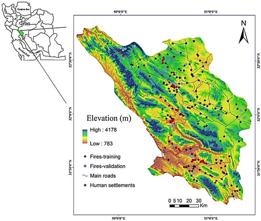
Remote Sens. 2019, 11, 618                                                                               2 of 18

attempts to satisfy a growing demand for fire prevention in the fire-prone landscapes [7]. These systems
are usually based on a predictive model which aims at providing near-time wildfire predictions up
to 10–15 years into the future [7,11].
      Given the investment of resources and time required to suppress wildfires, efficient and adaptable
techniques are needed to rapidly estimate the likelihood of fire occurrence. The first extensive works on
predicting wildfire probability date back to Chuvieco and Congalton [12] in Spain and De Vliegher [13]
in Greece, which were significantly elaborated by recent works [14–16], demonstrating that the future
wildfires tend to occur under similar local conditions that caused them in the past.
      Wildfire predictive modeling is typically performed in the following five steps [2,7,11,14–16]:
(1) Detecting and documenting historical fire events; (2) identifying a set of wildfire influencing
factors; (3) seeking the potential relationships between the influencing factors and the historical fires;
(4) elaborating a spatially explicit distribution map of wildfire probability; and (5) assessing the reliability
of the probability map and its utility for predicting the location of future fires. Over the past decades,
researchers mostly focused on step three of this methodology and evaluated various models in
an explicitly spatial way to fully explore the pattern of wildfire occurrences in response to different
geo-environmental factors [2,7,14–16]. Apart from the machine learning techniques that have emerged
in recent years [14,15], bivariate and multivariate methods have always been the most commonly
used modeling approaches [7,17,18]. While the machine learning techniques (e.g., artificial neural
networks, neuro-fuzzy, support vector machines, and decision trees) often enable the modelers/managers
to achieve a high level of predictive accuracy, their application requires a profound knowledge of
programming to adequately tune several hyper-parameters that control the model performance [16].
On the other hand, the bivariate (e.g., frequency ratio, weight of evidence, evidential belief function,
statistical index, and certainty factor) and multivariate (e.g., linear and logistic regressions) methods can
easily be performed with in an Excel spreadsheet and the other user-friendly interfaces and represent
a straightforward analytic framework [7,17–20]. These methods have been numerically formulated to
be easily used in different environmental settings and adapted to include updated datasets with low
complexity and computation costs. Based on the spatial relationships between input data, these models
predict the probability of occurrence (positive) or non-occurrence (negative) of a fire with probability
P(+) = 1 − P(−) [7,11,14].
      However, these models operate on different mathematical concepts (bivariate vs. multivariate)
that do not necessarily lead to the same performance in different environmental settings. For example,
Pourtaghi et al. [18] mapped forest fire susceptibility using the frequency ratio model and achieved
a predictive accuracy of 79.85%. Pourghasemi [17] used the evidential belief function and regression
logistic for mapping forest fire probability and reported predictive accuracies of 74.30 and 81.93%,
respectively. Jaafari et al. [7] and Hong et al. [19] employed the weight of evidence model
and demonstrated the capability of this model with predictive accuracies of 80.39% and 82.02%,
respectively. Nami et al. [20] used the evidential belief function and successfully mapped the wildfire
probability with a predictive accuracy of 81.03%. Most recently, Hong et al. [21] compared the weight
of evidence and regression logistic and reported predictive accuracies of 85.4 and 79.1%, respectively.
These reviews of the literature clearly indicate that there is no single best model that can be effectively
used in all fire-prone landscapes.
      Additionally, however, some researchers combined bivariate and multivariate methods toward
a more accurate predictive model and often achieved a significantly improved overall predictive
accuracy compared to the single models, as an integrated ensemble model offers higher capability
in the organization and description of data [16]. For example, in the context of landslide modeling,
Umar et al. [22] and Chen et al. [23] reported improved predictive accuracies for the integrated
frequency ratio-logistic regression and weight of evidence-logistic regression models compared to
the single frequency ratio and weight of evidence models. To date, however, such a modeling approach
has been rarely applied for wildfire prediction [24].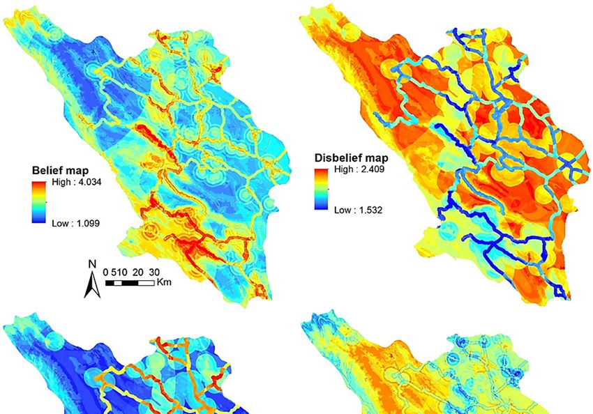
Remote Sens. 2019, 11, 618 3 of 18
In Iran, based on a report issued by the Forests, Range, and Watershed Management
Organization (FRWO), about 6000 ha of forests have been devastated by fires in 2017 alone.
Remote Sens. 2019, 11, x FOR PEER REVIEW 3 of 18
Particularly, the Zagros ecoregion in Western Iran is highly affected by frequent wildfires due to
its favorable climatic,
Particularly, biophysical,
the Zagros ecoregionand socioeconomic
in Western conditions
Iran is highly affected[20]. Investigations
by frequent wildfires ofdueinfluencing
to its
factors and the production of probability maps have been rarely performed for this
favorable climatic, biophysical, and socioeconomic conditions [20]. Investigations of influencing highly susceptible
ecoregion
factors [7,25]. In this study,
and the production we sought
of probability maps to
havebuild on these
been rarely effortsforby
performed thisusing
highlyand comparing
susceptible
ecoregion
evidential [7,25].
belief In this study,
function (EBF)we sought
and linearto build on these
regression efforts
(LR) by using
models to and
mapcomparing
wildfire evidential
probability in
belief function
a fire-prone landscape (EBF)ofand
thelinear regression
Zagros. (LR) models
The modeling to mapadopted
approach wildfire probability
in this study in aisfire-prone
motivated by
landscape of the Zagros. The modeling approach adopted in this study is
a desire to better explain the mechanisms responsible for wildfire occurrences in the Zagros motivated by a desire to
eco-region
better explain the mechanisms responsible for wildfire occurrences in the Zagros eco-region and to
and to understand the nature and capability of different models for treating the uncertainty inhered in
understand the nature and capability of different models for treating the uncertainty inhered in the
the spatial explicit modeling of wildfires.
spatial explicit modeling of wildfires.
2. Study Area
2. Study Area
This This
study
studywaswasconducted
conducted ininthe the central
central highlands
highlands of the ecoregion,
of the Zagros Zagros ecoregion,
Western Iran, Western
located Iran,
located between ◦ 0 ◦ 0 ◦ 0 ◦ 0
between 31°9′31N to9 32°48′
N to 32 48 N latitude
N latitude and 49°28′ and
E to4951°25′
28 EE to 51 25 (WGS
longitude E longitude
1984/UTM (WGSzone1984/UTM
39N)
zone (Figure
39N) (Figure 2 extent characterized by vegetation conditions ranging
1). The1). Thearea
study studyis aarea
16,532is akm
16,532 kmcharacterized
2 extent by vegetation conditions ranging from
fromgrasslands
grasslandstoto scatter forests
scatter dominated
forests dominated by Persian oak (Quercus
by Persian persica) [7].
oak (Quercus Topography
persica) varies widelyvaries
[7]. Topography
across the area (slope = 0–84°; ◦
widely across the area (slope = 0–84 ; altitude = 783–4178 m) and significantly affectslocal
altitude = 783–4178 m) and significantly affects the climate
the local climate
conditions. Annual rainfall varies from 1400 mm in the Northwest to 250
conditions. Annual rainfall varies from 1400 mm in the Northwest to 250 mm in the East and Southeast. mm in the East and
Southeast. Historically, winter and spring have been the wettest seasons of the year. The mean annual
Historically, winter and spring have been the wettest seasons of the year. The mean annual temperature
temperature ranges from 5 °C in the central parts to 16 °C in the Western parts, with an average of 10
ranges from 5 ◦ C in the central parts to 16 ◦ C in the Western parts, with an average of 10 ◦ C. Most of
°C. Most of the wildfires that occur in this area are caused due to decreased rainfall, drought
the wildfires that occur
occurrences, in this area
anthropogenic are causedor
phenomena, due to decreased
combinations rainfall,
thereof. drought
Despite theoccurrences,
frequency of anthropogenic
wildfires
phenomena, or combinations thereof. Despite the frequency of wildfires in
in this portion of the Zagros ecoregion, few studies have investigated the wildfire probability in this portion of thethis
Zagros
ecoregion, few
area [14]. studies have investigated the wildfire probability in this area [14].
1. 1.Location
Figure
Figure Locationof
of the studyarea
the study areaand
andhistorical
historical fires.
fires.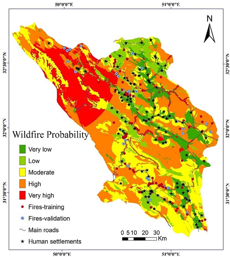
Remote Sens. 2019, 11, x618
                         FOR PEER REVIEW                                                                         44 of
                                                                                                                    of 18
                                                                                                                       18

3. Methodology
3. Methodology
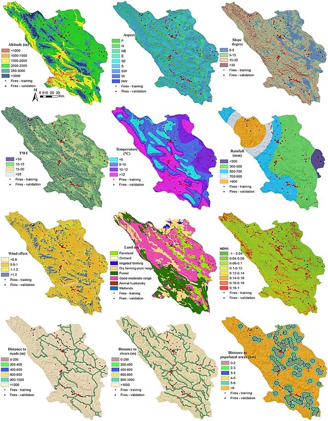
     The step by step workflow of the methodology adopted in this study is shown in Figure 2 and
     The (1)
includes  step  by step aworkflow
             compiling               of the methodology
                          wildfire inventory  map and a setadopted   in this study is shown invariables,
                                                              of the independent/explanatory      Figure 2
and  includes   (1) compiling   a wildfire inventory  map   and   a set of  the independent/explanatory
(2) multicollinearity assessment, (3) predictive modeling of wildfire occurrences using the EBF and
variables,
LR  models,(2)
             (4)multicollinearity  assessment,
                 validating and comparing    the(3) predictive
                                                 models,       modelingwildfire
                                                          (5) producing     of wildfire occurrences
                                                                                   probability  maps,using
                                                                                                      and
the EBF  and  LR  models,  (4) validating and comparing   the models,
(6) developing a probability map via an ensemble modeling approach.     (5) producing  wildfire probability
maps, and (6) developing a probability map via an ensemble modeling approach.

                          Figure 2.
                          Figure    Workflow of
                                 2. Workflow of the
                                                the methodology
                                                    methodology adopted
                                                                adopted in
                                                                        in this
                                                                           this study.
                                                                                study.

3.1. Wildfire Inventory
3.1. Wildfire Inventory
      An inventory of historical wildfires is the main basis for the statistical analyses of wildfire
     An inventory of historical wildfires is the main basis for the statistical analyses of wildfire
probabilities and can be conducted in different ways ranging from field surveys to interpretation
probabilities and can be conducted in different ways ranging from field surveys to interpretation of
of satellite imagery [15,20]. To prepare an inventory map of the wildfires that have occurred in
satellite imagery [15,20]. To prepare an inventory map of the wildfires that have occurred in the study
the study area, we first referred to the historical achieves to identify the spatial locations of the burnt
area, we first referred to the historical achieves to identify the spatial locations of the burnt areas in
areas in the recent past. We then used MODIS hot spot products (http://earthdata.nasa.gov/firms)
the recent past. We then used MODIS hot spot products (http://earthdata.nasa.gov/firms) and
and conducted several field surveys in various parts of the study area to verify the information of
conducted several field surveys in various parts of the study area to verify the information of
historical archives and produce a more reliable inventory map. Finally, we ended up with an inventory
historical archives and produce a more reliable inventory map. Finally, we ended up with an
map that consists of occurrence records of 137 fires for the period of 2007–2014 (Figure 1).
inventory map that consists of occurrence records of 137 fires for the period of 2007–2014 (Figure 1).
      Following previous works [2,7,14–21], we randomly sub-divided the wildfire locations into
     Following previous works [2,7,14–21], we randomly sub-divided the wildfire locations into
training and validation data subsets. The training dataset included 70% of the wildfires (1096 pixels)
training and validation data subsets. The training dataset included 70% of the wildfires (1096 pixels)
and the validation dataset included the remaining 30% of the wildfires (470 pixels).
and the validation dataset included the remaining 30% of the wildfires (470 pixels).
3.2. Independent Variables
3.2. Independent Variables
       An important task in wildfire predictive modeling is to identify the set of variables that carry
      An   important
complementary           task in wildfire
                     information.          predictive account
                                      To adequately    modeling  foris all
                                                                        to local
                                                                            identify  the set of variables
                                                                                  characteristics           that carry
                                                                                                   of the study    area,
complementary        information.   To  adequately    account   for   all  local  characteristics of the
twelve independent variables that have been frequently used in the wildfire literature were considered:   study   area,
twelve
Altitude, independent
             aspect, slopevariables    that have been
                             degree, topographic           frequently
                                                     wetness   index (TWI),used annual
                                                                                   in the temperature,
                                                                                           wildfire literature    were
                                                                                                         and rainfall,
considered:
wind effect, Altitude,
                land use, aspect,   slopedifference
                            normalized      degree, topographic     wetness
                                                     vegetation index           indexand
                                                                             (NDVI),    (TWI),  annual
                                                                                            distance to temperature,
                                                                                                        roads, rivers,
and   rainfall,  wind   effect, land  use, normalized   difference    vegetation     index  (NDVI),
and populated areas. We refer the interested reader to the corresponding literature [7,11,14–21,24]  and  distance to
roads,
for the rivers,   and populated
         information                 areas. Weofrefer
                         on the significance      thesethe  interested
                                                         variables         reader to
                                                                     on wildfire       the corresponding
                                                                                     occurrence              literature
                                                                                                 and their utility   for
[7,11,14–21,24]    for the  information    on the significance   of  these    variables  on wildfire
predictive modeling of future fires. To produce a topographic dataset describing altitude, aspect,   occurrence    and
their
slope,utility   for predictive
         and TWI,     we used amodeling       of futureModel
                                   Digital Elevation    fires. To
                                                                (DEM)produce     a topographic
                                                                            at 30-meter           dataset
                                                                                          resolution.  We describing
                                                                                                            processed
altitude,   aspect,  slope,  and  TWI,  we   used  a Digital  Elevation      Model   (DEM)   at 30-meter
the information obtained from the Meteorological Organization of the National Cartographic Center          resolution.
We processed the information obtained from the Meteorological Organization of the National
Cartographic Center of Iran to extract the maps of rainfall, temperature, wind effect, and distance to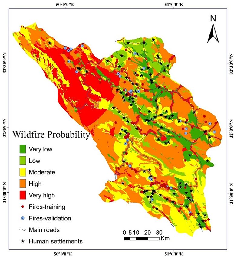
Remote Sens. 2019, 11, 618                                                                          5 of 18

Remote Sens. 2019, 11, x FOR PEER REVIEW                                                            5 of 18
of Iran to extract the maps of rainfall, temperature, wind effect, and distance to roads, rivers,
and  residential
roads,            areas.
        rivers, and       Furthermore,
                     residential         we generatedwe
                                 areas. Furthermore,    the land usethe
                                                          generated   andland
                                                                           NDVI
                                                                              usemaps   of themaps
                                                                                  and NDVI     studyofarea
                                                                                                       the
using
study Landsat-8
        area usingOLI   30 m (http://earthexplorer.usgs.gov).
                    Landsat-8                                   Finally, we categorized
                                OLI 30 m (http://earthexplorer.usgs.gov).   Finally, we each  explanatory
                                                                                         categorized each
variable  into variable
explanatory    several classes  based on
                         into several      the previous
                                        classes based on works [14–21,24,25]
                                                           the previous       and[14–21,24,25]
                                                                          works   local conditions
                                                                                                andoflocal
                                                                                                       our
study  landscape   (Figure 3).
conditions of our study landscape (Figure 3).

                             Figure 3.
                             Figure 3. Independent/explanatory
                                       Independent/explanatory variables
                                                               variables used
                                                                         used in
                                                                              in this
                                                                                 this study.
                                                                                      study.

3.3. Multicollinearity Assessment
     Most of the bivariate and multivariate techniques are sensitive to the inclusion of the collinear
variables, as these intercorrelated variables can significantly reduce the accuracy of the model [7].
Remote Sens. 2019, 11, 618                                                                                   6 of 18

3.3. Multicollinearity Assessment
     Most of the bivariate and multivariate techniques are sensitive to the inclusion of the collinear
variables, as these intercorrelated variables can significantly reduce the accuracy of the model [7].
Thus, before model building, the highly collinear variables should be identified and excluded from
further procedures [7–16]. To examine possible collinearity among the variables used in this study,
we computed the variance inflation factor (VIF) and tolerance and checked their critical values for all
variables. VIF > 5 or tolerance
Remote Sens. 2019, 11, 618                                                                                        7 of 18

3.5. Logistic Regression
     As the most popular multivariate statistical analysis method for the prediction of different
types of natural hazards [34], logistic regression (LR) is capable of exploring the spatial relationship
between an event (dependent variable) and an array of independent variables to elucidate
the underlying pattern of the occurrence of the event [34]. Since wildfire modeling is typically
formulated as a binary problem, LR builds a linear relationship between the dependent variable
and independent variables based on the presence (1) or absence (0) of fire. In this case, the model can
be given as:
                                   y = α + b1×1 + b2×2 + . . . + bn×n ,                               (7)
                                                              1
                                                    Pj =                                                             (8)
                                                           1 + e−y
where y is the probability of occurrence (1) or non-occurrence (0) of fire, α is the intercept of the model,
bi (i = 0, 1, 2, . . . , n) represents the model coefficients, xi (i = 0, 1, 2, . . . , n) donates the set of independent
variables, and Pj varies between 0 and 1 and is the probability of fire occurrence in each pixel of
the research landscape. The application of the LR model enables us to identify the most prominent
variables that best explain the spatial pattern of wildfire probability with in the landscape. All LR
calculations were performed using the SPSS software and were then transferred to ArcGIS software.

3.6. Ensemble Modeling
     To increase our chance for obtaining a more accurate estimate of wildfire probabilities, we followed
an ensemble modeling approach recommended in the literature [35] and combined the two probability
maps produced by the EBF and LR models, resulting in a single probability map that benefited from
the advantages of both EBF and LR models that alleviated some of the limitations of the basic models.
To do so, we used the raster calculator tool of the ArcGIS software and performed a simple raster
overlay. This operation resulted in combining characteristics for EBF and LR maps into a single
probability map.

3.7. Validation and Comparison
       The goodness-of-fit and predictive capability of the modeling approaches adopted in this study
were evaluated employing the receiver operating characteristic (ROC) curve and its two components,
i.e., sensitivity and specificity, that calculated the success rate and prediction rate and their associated
area under the curve (AUC). The philosophy and mathematical formulation of this method have been
fully presented in the corresponding literature [14–21]. In summary, the sensitivity (i.e., probability
of detection) answers the question of what fraction of the observed fire pixels are correctly classified,
and its perfect value is 1; specificity (i.e., negative predictive value) answers the question of what
fraction of the non-fire pixels are correctly classified, and its perfect value is 1. The ROC of the training
dataset yields the success rate of the model and measures the goodness-of-fit of the model. The ROC
of the validation dataset yields the prediction rate of the model and indicates how well or poorly
the model predicts the future events [7,14–21]. In terms of the AUC value, the values of 0.9 an excellent model
performance [36,37].
       To statistically compare the performance of the models, a pairwise comparison
between the probability indices extracted from each probability map was performed. This comparative
analysis was conducted using the Wilcoxon Signed-Rank Test (WSRT) [38], where the null
hypothesis assumes the performance of the models at the significance level of p = 0.05 is the same.
The −1.96 < z-value > 1.96 indicates that the p-value is less than 0.05 and rejects the null hypothesis.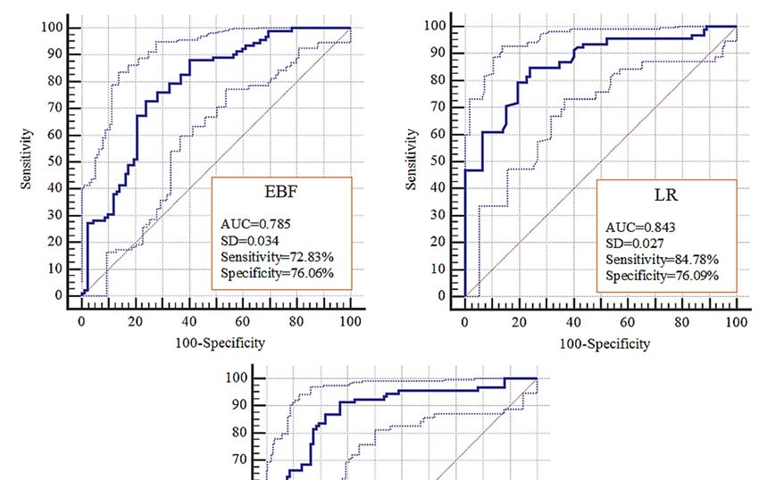
Remote Sens. 2019, 11, 618                                                                                                   8 of 18

4. Results and Discussion

4.1. Multicollinearity Assessment
     Our approach was to check and then to adequately select the predictive variables with the highest
predictive utility to build the models. Careful multicollinearity assessment is required to confidently
include the optimal subset of variables that make the greatest contribution to the likelihood of
Remote Sens. 2019, 11, x FOR PEER REVIEW                                                                     8 of 18
landslide occurrence [7,14,21]. In this study, the results of the multicollinearity assessment among
the variablesamong
assessment      showed    thethat no variable
                               variables      exceeded
                                         showed   that nothe criticalexceeded
                                                           variable   values of the
                                                                                VIFcritical
                                                                                     > 5 andvalues
                                                                                             TOL  5 and4).
Thus,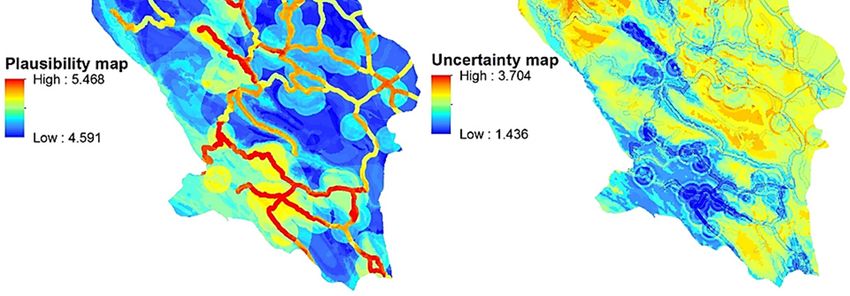
Remote Sens. 2019, 11, 618                                                                                  9 of 18

      Table 1. The spatial relationship between each predictor variable and wildfires extracted by using
      the evidential belief function (EBF) model.

                                 EBF Probability Mass                                EBF Probability Mass
     Variable        Class            Functions            Variable     Class             Functions
                               Bel    Dis    Unc    Pls                            Bel    Dis    Unc     Pls
                    0–1000     0.00   0.25   0.75   0.75                1.2       0.22   0.26   0.52    0.74
                   2500–3000   0.18   0.28   0.54   0.72
                    >3000      0.04   0.27   0.69   0.73                  L1       0.11   0.27   0.61    0.73
                                                                          L2       0.00   0.25   0.75    0.75
                       F       0.21   0.26   0.53   0.74                  L3       0.45   0.25   0.30    0.75
                      N        0.27   0.25   0.48   0.75   Land use       L4       0.41   0.23   0.36    0.77
                      NE       0.29   0.25   0.46   0.75                  L5       0.37   0.23   0.40    0.77
                      E        0.26   0.25   0.49   0.75                  L6       0.24   0.29   0.48    0.71
      Aspect
                      SE       0.36   0.24   0.40   0.76                  L7       0.00   0.25   0.75    0.75
                       S       0.25   0.26   0.49   0.74                  L8       0.00   0.25   0.75    0.75
                      SW       0.36   0.24   0.40   0.76
                      W        0.30   0.25   0.44   0.75               −1–0.04     0.21   0.26   0.53    0.74
                     NW        0.24   0.26   0.51   0.74               0.04–0.08   0.27   0.25   0.48    0.75
                                                                       0.08–0.1    0.29   0.25   0.46    0.75
                     0–5       0.23   0.27   0.50   0.73    NDVI       0.1–0.12    0.26   0.25   0.49    0.75
      Slope          5–15      0.39   0.21   0.40   0.79               0.12–0.14   0.36   0.24   0.40    0.76
      degree         15–30     0.34   0.23   0.43   0.77               0.14–0.16   0.25   0.26   0.49    0.74
                      >30      0.04   0.29   0.67   0.71               0.16–0.18   0.36   0.24   0.40    0.76
                                                                         0.18–1    0.30   0.25   0.44    0.75

                      20      0.11   0.26   0.64   0.74   Distance    400–600     0.65   0.24   0.10    0.76
                                                           to roads     600–800    0.97   0.23   -0.21   0.77
                      1000     0.22   0.60   0.18    0.40
       (◦ C)
                     10–12     0.26   0.26   0.48   0.74
                      >12      0.43   0.20   0.37   0.80                0–200      0.31   0.25   0.44    0.75
                                                                        200–400    0.21   0.26   0.54    0.74
                    1000
                                                                         0–2       0.62   0.23   0.15    0.77
                                                           Distance      2–3       0.44   0.24   0.32    0.76
                                                              to         3–4       0.55   0.23   0.22    0.77
                                                           populate      4–5       0.22   0.26   0.52    0.74
                                                            areas        5–6       0.38   0.24   0.37    0.76
                                                                         >6        0.18   0.39   0.43    0.61

     The final EBF map of wildfire probability was developed by integrating the four mass probability
maps and was reclassified into different probability levels representing the likelihoods of wildfire
occurrence across the study landscape (Figure 6). Visually, it is evident that the high and very
high levels of wildfire probability are highly associated with the road networks and forested areas.
These results are in close agreement with those who reported a positive association between human
activities and increased probability of fire occurrence [2,7]. However, if the EBF map is compared
to the uncertainty map (Figure 5), it is evident that the areas with high uncertainty correspond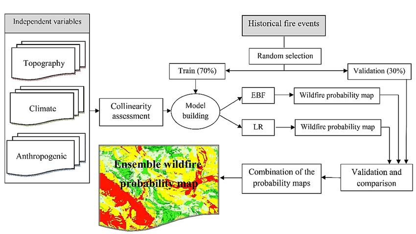
Remote Sens. 2019, 11, 618                                                                            10 of 18

to very low and low probability classes, although several fires have occurred in these portions of
the landscape. These results motivated us to consider an ensemble approach for treating the uncertainty
of the Sens.
Remote EBF 2019,
             model.
                 11, x FOR PEER REVIEW                                                           10 of 18

                 Figure 5. The index maps of the four probability mass
                                                                  mass functions
                                                                       functions of
                                                                                 of the
                                                                                    the EBF
                                                                                        EBF model.
                                                                                            model.

       The model parameters resulting from the application of the LR model are shown in Table 2.
The final LR model for the training dataset retained only five (i.e., slope, rainfall, land use, and distance
to populated areas and roads) of the twelve original variables (Table 3). The regression coefficient
(ß) of the selected variables indicate the magnitude to which these variables exert an effect on
the probability of wildfire occurrences in the research landscape; chief among them was the land use
variable. This variable was used here as a proxy for human influences on the spatial pattern of wildfire
probabilities [2,7,11,20,21] that delineated zones of similar conditions in terms of human-ignition
patterns, indicating that dry farmlands and forests are the most susceptible portions of the landscape to
fire occurrences. During field surveys, we found that while human activities predominantly controlled
the distribution of all fires throughout the landscape, the type and contiguous patches of vegetation
(i.e., fuel sources for fires) mainly determined the incidence of the largest fires.

               Figure 6. The distribution map of wildfire probability produced using the EBF model.
Remote Sens. 2019, 11, 618 11 of 18
Figure 5. The index maps of the four probability mass functions of the EBF model.
Figure 6.
Figure The distribution
6. The distribution map
map of
of wildfire
wildfire probability produced using the EBF model.
Table 2. Summary of the implementation of the logistic regression (LR) model.
Step Chi-Square −2 Log Likelihood Cox & Snell R Square Nagelkerke R Square
1 2.532 240.749a 0.075 0.100
2 7.617 235.434a 0.101 0.135
3 15.880 224.975a 0.151 0.201
4 13.302 220.813a 0.170 0.227
5 16.484 215.842b 0.192 0.256
a. Estimation terminated at iteration number 4 because parameter estimates changed by less than 0.001. b. Estimation
terminated at iteration number 5 because parameter estimates changed by less than 0.001.
Table 3. Variable coefficients extracted using the LR model.
95% C.I. for EXP(B)
Exp (ß) Sig. df Wald S.E ß Variables in the Equation
Upper Lower
0.897 0.373 0.579 0.14 1 5.979 0.224 −0.547 Slope Step 5
0.932 0.454 0.650 0.019 1 5.497 0.183 0.430 Rainfall
0.589 0.032 0.137 0.008 1 7.113 0.745 −1.990 Land use (Farmland)
25.499 0.009 0.475 0.714 1 0.134 2.032 −0.744 Land use (Orchard)
5.442 0.926 2.245 0.703 1 3.206 0.452 0.809 Land use (Dry farming)
5.050 0.942 2.182 0.069 1 3.317 0.428 0.780 Land use (Forest)
0.977 0.667 0.807 0.028 1 4.828 0.097 −0.214 Dis. to populated areas
0.896 0.534 0.691 0.005 1 7.814 0.132 −0.369 Dis. to roads
165.936 0.000 1 20.194 1.137 −5.112 Constant
S.E: Standard Error of estimate; Wald: Wald chi-square values; df: Degree of freedom; Sig: Significance value.Remote Sens. 2019, 11, 618 12 of 18
The negative coefficients for the slope and distance factors indicate that these variables are of little
importance for the probability of fire occurrence (Table 3). Using these coefficients and Equation (7),
the wildfire probability values for the entire study region were generated as follows:
Y = ((−5.112) + (Slope × −0.547) + (Rainfall × 0.430) + (Farmland × −1.990) + (Orchard × −0.744)
+ (Dry farming × 0.809) + (Forest × 0.780) + (Distance to populated areas × −0.214)
(9)
+ (Distance to roads × −0.369))
Figure 7 shows the observed groups (1 (non-fire) and 2 (fire)) and the predicted probabilities
of the pixels used in the LR model. The appropriate bunching of the observations towards the left
and right ends of the graph demonstrates that the LR model performed reasonably well at classifying
the training dataset into fires and non-fires. The final LR map of wildfire probability was developed by
transferring the 2019,
Remote Sens. probability values
11, x FOR PEER to the ArcGIS software (Figure 8).
REVIEW 12 of 18
Remote Sens. 2019, 11, x FOR PEER REVIEW 12 of 18
FigureFigure
Figure7.7.Observed
7. Observed
Observed groups
groups
groupsand
and predicted
predictedprobabilities
predicted
and probabilitiesextracted
probabilities using
extracted
extracted the
theLR
using
using model.
the
LR LR model.
model.
FigureFigure 8.8.distribution
8. The
Figure The
Thedistribution map
map
distribution ofofofwildfire
map wildfire
wildfireprobability
probabilityproduced
probability using
produced
produced the
theLR
using
using model.
the
LR LR model.
model.
Upon
Uponproducing
producingthethewildfire
wildfireprobability
probabilitymaps
mapsusing
usingthe
theEBF
EBFand
andLRLRmodels,
models,the
thetwo
twomaps
mapswere
were
combined
combined to achieve an ensemble map of wildfire probability (Figure 9). This operation resulted in
to achieve an ensemble map of wildfire probability (Figure 9). This operation resulted in
combining
combiningcharacteristics
characteristicsfor
forEBF
EBFand
andLR
LRmaps
mapsinto
intoaasingle
singleprobability
probabilitymap.
map.Remote Sens. 2019, 11, 618 13 of 18
Upon producing the wildfire probability maps using the EBF and LR models, the two maps were
combined to achieve an ensemble map of wildfire probability (Figure 9). This operation resulted in
combining
Remote characteristics
Sens. 2019, forREVIEW
11, x FOR PEER EBF and LR maps into a single probability map. 13 of 18
Figure 9.
Figure The ensemble
9. The ensemble (EBF-LR)
(EBF-LR) wildfire
wildfire probability
probability map.
4.3. Validation
4.3. Validation andand Comparision
Comparision
The three
The three wildfire
wildfireprobability
probabilitymaps mapsproduced
produced byby thethe three
three models
models werewere compared
compared usingusing
the
the success rates (Figure 10) and prediction rates (Figure 11). In the case
success rates (Figure 10) and prediction rates (Figure 11). In the case of the EBF and LR models, LR of the EBF and LR models,
LR showed
showed the the greatest
greatest goodness-of-fit
goodness-of-fit with
with thethe training
training dataset(AUC
dataset (AUC= =0.843)
0.843)and
andthe
thecapability
capability to to
predict future fires (AUC = 0.728). In the literature, EBF and LR models
predict future fires (AUC = 0.728). In the literature, EBF and LR models were used either separatelywere used either separately [20]
or compared
[20] or compared to other models
to other [17]. [17].
models While the EBF
While model
the EBF proved
model itselfitself
proved to betorather simple
be rather and easy
simple and
to apply [20], the LR model appears more complex, as this model
easy to apply [20], the LR model appears more complex, as this model requires the modelers requires the modelers to convertto
the data from the GIS standard format to the format required by
convert the data from the GIS standard format to the format required by the statistical software the statistical software [17,21].
However,
[17,21]. despitedespite
However, the LRthe thatLRaccepts both discrete
that accepts and continuous
both discrete and continuous inputs, EBFEBF
inputs, onlyonly
operates
operates on
discrete-form inputs.
on discrete-form inputs.
Applying the
Applying the ensemble
ensemble approach,
approach, we we achieved
achieved an an improved
improved model model performance
performance in in both
both training
training
(AUC = 0.898) and validation (AUC = 0.864) datasets compared to those
(AUC = 0.898) and validation (AUC = 0.864) datasets compared to those obtained using the LR and obtained using the LR and EBF
models. The capability of hybrid and ensemble approaches for
EBF models. The capability of hybrid and ensemble approaches for improving the predictive improving the predictive accuracy of
natural phenomena
accuracy has been widely
of natural phenomena acknowledged
has been in previous works
widely acknowledged [16,35,36,39].
in previous In a recent work,
works [16,35,36,39]. In a
Hong et al. [21] proposed an integrated model that relied on the weight
recent work, Hong et al. [21] proposed an integrated model that relied on the weight of evidence of evidence and the analytical
and
hierarchy
the process
analytical and demonstrated
hierarchy a significantlyaimproved
process and demonstrated significantly prediction
improved of future fires.of
prediction The ensemble
future fires.
wildfire probability map developed in this study takes the advantages
The ensemble wildfire probability map developed in this study takes the advantages of both LR and of both LR and EBF models that
successfully measured the importance of each variable and its
EBF models that successfully measured the importance of each variable and its categories.categories.
The results
The results of ofthe
thecomparison
comparisonofofthe the success
success rates
rates using
using thetheWSRT WSRT (Table
(Table 4) indicate
4) indicate that that
the
the training performance of the models differed significantly, as
training performance of the models differed significantly, as z- and p-values for the pairwise z- and p-values for the pairwise
comparisons exceeded
comparisons exceeded the the critical
critical values.
values. Additionally,
Additionally, the the same
same results
results were
were achieved
achieved by by comparing
comparing
the prediction
the prediction ratesrates (Table
(Table 5),
5), indicating
indicating thatthat the
the capability
capability of of the
the models
models to to predict
predict wildfires
wildfires differed
differed
significantly. While the EBF model can adequately explore the spatial associations between a
variables class and past wildfires, the model fails to rank the variables and generally assumes equal
weights for all variables [20]. This is due to the general philosophy of a bivariate model that
investigates the significance of several variables separately [16].
Although in this study the multivariate LR model performed much better than the bivariate EBFRemote Sens. 2019, 11, 618 14 of 18
significantly. While the EBF model can adequately explore the spatial associations between a variables
class and past wildfires, the model fails to rank the variables and generally assumes equal weights
for all variables [20]. This is due to the general philosophy of a bivariate model that investigates
the significance of several variables separately [16].
Remote Although inxthis
Sens. 2019, 11, FORstudy the multivariate LR model performed much better than the bivariate
PEER REVIEW EBF
14 of 18
model, LR has been frequently criticized due to its basic algorithm that considers a linear relationship
between
betweenaaphenomenon
phenomenonand andits
itscausal
causalfactors
factors[21,34]
[21,34]that
thatactually
actuallydoes
doesnotnotmeet
meetthe
thecomplex
complexnaturenature
of natural hazards [16,39]. In this context, some studies even suggest
of natural hazards [16,39]. In this context, some studies even suggest that the LR model tends that the LR model tends to
underestimate the probability of occurrence of an event [40].
to underestimate the probability of occurrence of an event [40]. However, some other studies However, some other studies
demonstrated
demonstratedthat thatthe
thebivariate
bivariatemodels
modelsare arehighly
highlysensitive
sensitivetotothe
thequality
qualityof ofinput
inputdata
dataandandoften
oftenfail
fail
to fully explore the real relationships between wildfires and their drivers [7,20].
to fully explore the real relationships between wildfires and their drivers [7,20]. On the other hand, On the other hand,
some researchersbelieve
some researchers believe thatthat different
different methods methods have
have their owntheir ownadvantages
intrinsic intrinsic andadvantages
disadvantagesand
disadvantages
and it is not true and it isa not
that true
single that aissingle
model modelsuperior
absolutely is absolutely
to thesuperior to the others [14,41].
others [14,41].
With
With the increasing frequency and intensity of wildfires, it becomesmore
the increasing frequency and intensity of wildfires, it becomes moreandandmore
moreimportant
important
to
tobuild
buildand andsuggest
suggest accurate
accuratepredictive models.
predictive Approaches
models. integrating
Approaches multiplemultiple
integrating individual models
individual
can provide robust estimates of future fires [16,21,24]. Given the proven
models can provide robust estimates of future fires [16,21,24]. Given the proven capability of capability of the ensemble
approach
the ensemble adopted
approachin this study,
adopted in we
this can
study,conclude that the that
we can conclude singletheapplication of bivariate
single application and
of bivariate
multivariate
and multivariatemodels is inefficient
models and outdated,
is inefficient highlighting
and outdated, the need the
highlighting to update
need to their basic structures
update their basic
toward an advanced model. Thus, in line with the efforts devoted
structures toward an advanced model. Thus, in line with the efforts devoted to developingto developing new models for new
the
prediction of landslides [39] and floods [42], further research is needed
models for the prediction of landslides [39] and floods [42], further research is needed to improve to improve the wildfire
prediction
the wildfiremodels
predictionandmodels
the ability
and the of ability
managers and authorities
of managers for making
and authorities more more
for making informed fire
informed
presentation and suppression decisions.
fire presentation and suppression decisions.
Figure 10. Success rate curves of the three models.
Figure 10. Success rate curves of the three models.Remote Sens. 2019, 11, 618 15 of 18
Remote Sens. 2019, 11, x FOR PEER REVIEW 15 of 18
Figure 11.
Figure Prediction rate
11. Prediction rate curves
curves of
of the
the three
three models.
models.
Table 4. Pairwise comparison of the models’ success rates using the Wilcoxon Signed-Rank Test (WSRT).
Table 4. Pairwise comparison of the models’ success rates using the Wilcoxon Signed-Rank Test
(WSRT). z-Value p-Value Sig.
EBF vs. LR 11.463 p < 0.0001 Yes
z-Value p-Value Sig.
EBF vs. EBF-LR −11.763 p < 0.0001 Yes
EBF
LR vs.vs. LR
EBF-LR −11.463
11.764 ppRemote Sens. 2019, 11, 618 16 of 18
combining two probability maps. The results of this map combination clearly revealed that the EBF
and LR models act very well in conjunction with each other and can significantly improve the ability
to predict future wildfires. More generally, further research is required to understand the nature of
different models and to understand what characteristics motivate modelers to select a model or not.
Understanding these characteristics can help modelers and managers in ways that provide an accurate
estimate of wildfire probability in reasonable computation time. Future research must provide explicit
information about model selection based on predictive capability, ideally using a more inclusive
range of independent variables and powerful data collection methods that will capture landscape
characteristics realistically.
Author Contributions: Conceptualization, A.J. and D.M.-G.; data acquisition, D.M.-G.; methodology, A.J.,
D.M.-G., B.T.P., and D.T.B.; writing—original draft preparation, A.J.; writing—review and editing, A.J., D.M.-G.,
B.T.P., and D.T.B.; APC, B.T.P. and D.T.B.
Funding: This research was partially funded by University of South-Eastern Norway.
Conflicts of Interest: The authors declare no conflict of interest.
References
1. Pacheco, A.P.; Claro, J.; Fernandes, P.M.; de Neufville, R.; Oliveira, T.M.; Borges, J.G.; Rodrigues, J.C. Cohesive
fire management with in an uncertain environment: A review of risk handling and decision support systems.
Ecol. Manag. 2015, 347, 1–17. [CrossRef]
2. Pourtaghi, Z.S.; Pourghasemi, H.R.; Aretano, R.; Semeraro, T. Investigation of general indicators influencing
on forest fire and its susceptibility modeling using different data mining techniques. Ecol. Indic. 2016,
64, 72–84. [CrossRef]
3. Bowman, D.M.; Balch, J.K.; Artaxo, P.; Bond, W.J.; Carlson, J.M.; Cochrane, M.A.; D’Antonio, C.M.;
De Fries, R.S.; Doyle, J.C.; et al. Fire in the Earth system. Science 2009, 324, 481–484. [CrossRef] [PubMed]
4. Meng, Y.; Deng, Y.; Shi, P. Mapping Forest Wildfire Risk of the World. In World Atlas of Natural Disaster Risk;
Springer: Berlin/Heidelberg, Germany, 2015; pp. 261–275.
5. Calder, W.J.; Shuman, B. Extensive wildfires, climate change, and an abrupt state change in subalpine ribbon
forests, Colorado. Ecology 2017, 98, 2585–2600. [CrossRef]
6. Stevens-Rumann, C.S.; Kemp, K.B.; Higuera, P.E.; Harvey, B.J.; Rother, M.T.; Donato, D.C.; Morgan, P.;
Veblen, T.T. Evidence for declining forest resilience to wildfires under climate change. Ecol. Lett. 2018,
21, 243–252. [CrossRef] [PubMed]
7. Jaafari, A.; Mafi-Gholami, D.; Zenner, E.K. A Bayesian modeling of wildfire probability in the Zagros
Mountains, Iran. Ecol. Inf. 2017, 39, 32–44. [CrossRef]
8. Petty, A.M.; Isendahl, C.; Brenkert-Smith, H.; Goldstein, D.J.; Rhemtulla, J.M.; Rahman, S.A.; Kumasi, T.C.
Applying historical ecology to natural resource management institutions: Lessons from two case studies of
landscape fire management. Glob. Environ. Chang. 2015, 31, 1–10. [CrossRef]
9. Pettit, N.E.; Naiman, R.J.; Warfe, D.M.; Jardine, T.D.; Douglas, M.M.; Bunn, S.E.; Davies, P.M.
Productivity and connectivity in tropical riverscapes of northern Australia: Ecological insights for management.
Ecosystems 2017, 20, 492–514. [CrossRef]
10. Monedero, S.; Ramirez, J.; Cardil, A. Predicting fire spread and behaviour on the fireline. Wildfire analyst
pocket: A mobile app for wildland fire prediction. Ecol. Model. 2019, 392, 103–107. [CrossRef]
11. Ngoc-Thach, N.; Ngo, D.B.T.; Xuan-Canh, P.; Hong-Thi, N.; Thi, B.H.; NhatDuc, H.; Dieu, T.B. Spatial pattern
assessment of tropical forest fire danger at Thuan Chau area (Vietnam) using GIS-based advanced machine
learning algorithms: A comparative study. Ecol. Inf. 2018, 48, 74–85. [CrossRef]
12. Chuvieco, E.; Congalton, R.G. Application of remote sensing and geographic information systems to forest
fire hazard mapping. Rem. Sens. Env. 1989, 29, 147–159. [CrossRef]
13. De Vliegher, B.M. Risk assessment for environmental degradation caused by fires using remote sensing
and GIS in a Mediterranean Region (South-Euboia, Central Greece). In Proceedings of the International
IGARSS’92 Geoscience and Remote Sensing Symposium, Houston, TX, USA, 26–29 May 1992; Volume 1,
pp. 44–47.Remote Sens. 2019, 11, 618 17 of 18
14. Jaafari, A.; Zenner, E.K.; Pham, B.T. Wildfire spatial pattern analysis in the Zagros Mountains, Iran:
A comparative study of decision tree based classifiers. Ecol. Inf. 2018, 43, 200–211. [CrossRef]
15. Tien Bui, D.; Le, K.T.T.; Nguyen, V.C.; Le, H.D.; Revhaug, I. Tropical forest fire susceptibility mapping at the
cat Ba national park area, Hai Phong city, Vietnam, using GIS-Based kernel logistic regression. Remote Sens.
2016, 8, 347. [CrossRef]
16. Jaafari, A.; Zenner, E.K.; Panahi, M.; Shahabi, H. Hybrid artificial intelligence models based on a neuro-fuzzy
system and metaheuristic optimization algorithms for spatial prediction of wildfire probability. Agric. For. Meteorol.
2019, 266, 198–207. [CrossRef]
17. Pourghasemi, H.R. GIS-based forest fire susceptibility mapping in Iran: A comparison between evidential
belief function and binary logistic regression models. Scand. J. For. Res. 2016, 31, 80–98. [CrossRef]
18. Pourtaghi, Z.S.; Pourghasemi, H.R.; Rossi, M. Forest fire susceptibility mapping in the Minudasht forests,
Golestan province, Iran. Environ. Earth Sci. 2015, 73, 1515–1533. [CrossRef]
19. Hong, H.; Naghibi, S.A.; Dashtpagerdi, M.M.; Pourghasemi, H.R.; Chen, W. A comparative assessment
between linear and quadratic discriminant analyses (LDA-QDA) with frequency ratio and weights-of-evidence
models for forest fire susceptibility mapping in China. Arab. J. Geosci. 2017, 10, 167. [CrossRef]
20. Nami, M.H.; Jaafari, A.; Fallah, M.; Nabiuni, S. Spatial prediction of wildfire probability in the Hyrcanian
ecoregion using evidential belief function model and GIS. Int. J. Environ. Sci. Technol. 2018, 15, 373–384.
[CrossRef]
21. Hong, H.; Jaafari, A.; Zenner, E.K. Predicting spatial patterns of wildfire susceptibility in the Huichang
County, China: An integrated model to analysis of landscape indicators. Ecol. Indic. 2019, 101, 878–891.
[CrossRef]
22. Umar, Z.; Pradhan, B.; Ahmad, A.; Jebur, M.N.; Tehrany, M.S. Earthquake induced landslide susceptibility
mapping using an integrated ensemble frequency ratio and logistic regression models in West Sumatera
Province, Indonesia. Catena 2015, 118, 124–135. [CrossRef]
23. Chen, W.; Sun, Z.; Han, J. Landslide susceptibility modeling using integrated ensemble weights of evidence
with logistic regression and random forest models. Appl. Sci. 2019, 9, 171. [CrossRef]
24. Tien Bui, D.; Bui, Q.T.; Nguyen, Q.P.; Pradhan, B.; Nampak, H.; Trinh, P.T. A hybrid artificial intelligence
approach using GIS-based neural-fuzzy inference system and particle swarm optimization for forest fire
susceptibility modeling at a tropical area. Agric. For. Meteorol. 2017, 233, 32–44. [CrossRef]
25. Jaafari, A.; Pourghasemi, H.R. Factors Influencing Regional Scale Wildfire Probability in Iran: An Application
of Random Forest and Support Vector Machine. In Modeling in GIS and R for Earth and Environmental Science;
Pourghasemi, H.R., Candan, G., Eds.; Elsevier: Amsterdam, The Netherlands, 2019.
26. Tehrany, M.S.; Kumar, L. The application of a Dempster–Shafer-based evidential belief function in flood
susceptibility mapping and comparison with frequency ratio and logistic regression methods. Environ. Earth Sci.
2018, 77, 490. [CrossRef]
27. Dempster, A.P. Upper and lower probabilities induced by a multivalued mapping. Ann. Math. Stat. 1967,
38, 325–339. [CrossRef]
28. Dempster, A.P. Upper and lower probability inferences based on a sample from a finite univariate population.
Biometrika 1967, 54, 515–528. [CrossRef] [PubMed]
29. Shafer, G.A. Mathematical Theory of Evidence; Princeton University Press: Princeton, NJ, USA, 1976; 297p.
30. Carranza, E.J.M.; Van Ruitenbeek, F.; Hecker, C.; van der Mejide, M.; van der Meer, F.D. Knowledge-guided
data-driven evidential belief modeling of mineral prospectivity in Cabo de Gata, SE Spain. Int. J. Appl. Earth Obs.
2008, 10, 374–387. [CrossRef]
31. Naghibi, S.A.; Pourghasemi, H.R.; Dixon, B. GIS-based groundwater potential mapping using boosted
regression tree, classification and regression tree, and random forest machine learning models in Iran.
Environ. Monit. Assess. 2016, 188, 1–27. [CrossRef] [PubMed]
32. Carranza, E.J.M.; Woldai, T.; Chikambwe, E.M. Application of data-driven evidential belief functions to
prospectivity mapping for aquamarine-bearing pegmatites, Lundazi district, Zambia. Nat. Resour. Res. 2005,
14, 47–63. [CrossRef]
33. Gorum, T.; Carranza, E.J.M. Control of style-of-faulting on spatial pattern of earthquake-triggered landslides.
Int. J. Environ. Sci. Technol. 2015, 12, 3189–3212. [CrossRef]
34. Pham, B.T.; Prakash, I.; Jaafari, A.; Bui, D.T. Spatial prediction of rainfall-induced landslides using
aggregating one-dependence estimators classifier. J. Ind. Soc. Remote Sens. 2018, 46, 1457–1470. [CrossRef]Remote Sens. 2019, 11, 618 18 of 18
35. Choubin, B.; Moradi, E.; Golshan, M.; Adamowski, J.; Sajedi-Hosseini, F.; Mosavi, A. An Ensemble
prediction of flood susceptibility using multivariate discriminant analysis, classification and regression trees,
and support vector machines. Sci. Total. Environ. 2019, 651, 2087–2096. [CrossRef] [PubMed]
36. Jaafari, A. LiDAR-supported prediction of slope failures using an integrated ensemble weights-of-evidence
and analytical hierarchy process. Environ. Earth Sci. 2018, 77, 42. [CrossRef]
37. Hanley, J.A.; McNeil, B.J. The meaning and use of the area under a receiver operating characteristic (ROC)
curve. Radiology 1982, 143, 29–36. [CrossRef] [PubMed]
38. Wilcoxon, F. Individual comparisons by ranking methods. Biom. Bull. 1945, 1, 80–83. [CrossRef]
39. Jaafari, A.; Panahi, M.; Pham, B.T.; Shahabi, H.; Bui, D.T.; Rezaie, F.; Lee, S. Meta optimization of an adaptive
neuro-fuzzy inference system with grey wolf optimizer and biogeography-based optimization algorithms
for spatial prediction of landslide susceptibility. Catena 2019, 175, 430–445. [CrossRef]
40. Zhu, A.X.; Miao, Y.; Wang, R.; Zhu, T.; Deng, Y.; Liu, J.; Yang, L.; Cheng-Zhi, Q.; Hong, H. A comparative
study of an expert knowledge-based model and two data-driven models for landslide susceptibility mapping.
Catena 2018, 166, 317–327. [CrossRef]
41. Tutmez, B.; Ozdogan, M.G.; Boran, A. Mapping forest fires by nonparametric clustering analysis. J. For. Res.
2018, 29, 177–185. [CrossRef]
42. Termeh, S.V.R.; Kornejady, A.; Pourghasemi, H.R.; Keesstra, S. Flood susceptibility mapping using novel
ensembles of adaptive neuro fuzzy inference system and metaheuristic algorithms. Sci. Total Environ. 2018,
615, 438–451. [CrossRef]
© 2019 by the authors. Licensee MDPI, Basel, Switzerland. This article is an open access
article distributed under the terms and conditions of the Creative Commons Attribution
(CC BY) license (http://creativecommons.org/licenses/by/4.0/).You can also read


