The importance of considering sub-grid cloud variability when using satellite observations to evaluate the cloud and precipitation simulations in ...
←
→
Page content transcription
If your browser does not render page correctly, please read the page content below
Geosci. Model Dev., 11, 3147–3158, 2018
https://doi.org/10.5194/gmd-11-3147-2018
© Author(s) 2018. This work is distributed under
the Creative Commons Attribution 4.0 License.

The importance of considering sub-grid cloud variability when
using satellite observations to evaluate the cloud and precipitation
simulations in climate models
Hua Song1 , Zhibo Zhang1,2 , Po-Lun Ma3 , Steven Ghan3 , and Minghuai Wang4
1 Joint Center for Earth Systems Technology, UMBC, Baltimore, MD, USA
2 Physics  Department, UMBC, Baltimore, MD, USA
3 Atmospheric Sciences and Global Change Division, Pacific Northwest National Laboratory, Richland, WA, USA
4 Institute for Climate and Global Change Research & School of Atmospheric Sciences, Nanjing University, Nanjing, China

Correspondence: Zhibo Zhang (zhibo.zhang@umbc.edu)

Received: 19 January 2018 – Discussion started: 12 February 2018
Revised: 18 May 2018 – Accepted: 29 May 2018 – Published: 3 August 2018

Abstract. Satellite cloud observations have become an in-           ences between the two COSP runs demonstrate that it is im-
dispensable tool for evaluating general circulation mod-            portant to take into account the sub-grid variations of cloud
els (GCMs). To facilitate the satellite and GCM compar-             and precipitation when using COSP to evaluate the GCM to
isons, the CFMIP (Cloud Feedback Model Inter-comparison             avoid confusing and misleading results.
Project) Observation Simulator Package (COSP) has been
developed and is now increasingly used in GCM evalua-
tions. Real-world clouds and precipitation can have signifi-
cant sub-grid variations, which, however, are often ignored         1   Introduction
or oversimplified in the COSP simulation. In this study, we
use COSP cloud simulations from the Super-Parameterized             Marine boundary layer (MBL) cloud, as a strong modulator
Community Atmosphere Model (SPCAM5) and satellite ob-               of the radiative energy budget of the Earth–atmosphere sys-
servations from the Moderate Resolution Imaging Spectro-            tem, is a major source of uncertainty in future climate change
radiometer (MODIS) and CloudSat to demonstrate the im-              projections of the general circulation models (GCMs) (Cess
portance of considering the sub-grid variability of cloud and       et al., 1996; Bony and Dufresne, 2005). Improving MBL
precipitation when using the COSP to evaluate GCM simu-             cloud simulations in the GCMs is one of the top priorities
lations. We carry out two sensitivity tests: SPCAM5 COSP            of the climate modeling community. As the cloud param-
and SPCAM5-Homogeneous COSP. In the SPCAM5 COSP                     eterization schemes in the GCMs become increasingly so-
run, the sub-grid cloud and precipitation properties from the       phisticated, there is a strong need for comprehensive global
embedded cloud-resolving model (CRM) of SPCAM5 are                  satellite cloud observations for model evaluation and im-
used to drive the COSP simulation, while in the SPCAM5-             provement. However, the fundamental definitions of clouds
Homogeneous COSP run only grid-mean cloud and precipi-              in GCMs differ dramatically from those used for satellite re-
tation properties (i.e., no sub-grid variations) are given to the   mote sensing, which hampers the use of satellite products
COSP. We find that the warm rain signatures in the SPCAM5           for model evaluation. In order to overcome this obstacle, the
COSP run agree with the MODIS and CloudSat observations             Cloud Feedback Model Intercomparison Project (CFMIP)
quite well. In contrast, the SPCAM5-Homogeneous COSP                community has developed an integrated satellite simulator,
run which ignores the sub-grid cloud variations substantially       the CFMIP Observation Simulator Package (COSP) (Zhang
overestimates the radar reflectivity and probability of precip-     et al., 2010; Bodas-Salcedo et al., 2011). COSP has greatly
itation compared to the satellite observations, as well as the      facilitated and promoted the use of satellite data in the cli-
results from the SPCAM5 COSP run. The significant differ-           mate modeling community to expose and diagnose issues in

Published by Copernicus Publications on behalf of the European Geosciences Union.
3148                                          H. Song et al.: Importance of sub-grid cloud variability for model evaluation

GCM cloud simulations (e.g., Marchand et al., 2009; Zhang         sub-grid cloud and precipitation variability in the COSP sim-
et al., 2010; Kay et al., 2012, 2016; Pincus et al., 2012; Song   ulations.
et al., 2018).                                                       The current version (v1.4) of COSP provides a built-in
   Warm rain is a unique and important feature of MBL             highly simplified sub-column generator. It accounts only
clouds. It plays an important role in determining the macro-      for the sub-grid variability of the types of hydrometeors
and micro-physical properties of MBL clouds, in particular,       and ignores the variability of mass and microphysics within
the cloud water budget (e.g., Stevens et al., 2005; Wood,         each hydrometeor type. The water content and microphysical
2005; Comstock et al., 2005). Many previous studies have          properties (i.e., droplet effective radius and optical thickness)
investigated the warm rain simulation in GCMs using the           of each hydrometeor are horizontally homogenous among all
COSP simulators. These studies reveal a common problem            the sub-columns that are labeled as the same type (i.e., strat-
in the latest generation of GCMs; i.e., the drizzle in MBL        iform or convective). Here we refer to the current scheme
clouds is too frequent in the GCM compared with satellite         as the “homogenous hydrometeor scheme”. The uncertainties
observations (e.g., Zhang et al., 2010; Franklin et al., 2013;    and potential biases caused by the homogenous hydrometeor
Suzuki et al., 2015; Takahashi et al., 2017; Jing et al., 2017;   scheme can be significant and should not be overlooked. A
Song et al., 2017; Bodas-Salcedo et al., 2008, 2011; Stephens     simple hypothetical example is provided in Fig. 1 to illus-
et al., 2012; Nam and Quaas, 2012; Franklin et al., 2013; Jing    trate the importance of accounting for the sub-grid variabil-
et al., 2017). One possible reason for the excessive warm rain    ity of rainwater in simulating the CloudSat radar reflectivity.
production in GCMs could be the model’s inaccurate repre-         To be consistent with the two-moment cloud microphysics
sentation of physical processes, such as auto-conversion and      scheme (Morrison and Gettelman, 2008) that is widely used
accretion, that govern the precipitation efficiency in warm       in the GCMs, we assume the sub-grid distribution of rainwa-
MBL clouds. Due to the lack of sub-grid variability of mi-        ter to follow the exponential distribution. In this example, the
crophysical quantities in most large-scale models, the auto-      grid-mean rainwater mixing ratio (q̄) is set to be 0.03 g kg−1
conversion parameterization is overly aggressive, so that the     (dashed blue line in Fig. 1a). Using the Quickbeam simulator
models tend to produce precipitation too quickly (Lebsock et      (Haynes et al., 2007) in COSP, we simulated the correspond-
al., 2013; Song et al., 2017).                                    ing 94 GHz CloudSat radar reflectivity, which is shown in
   The radar observations of warm rain from CloudSat and          Fig. 1b. The grid-mean radar reflectivity based on the expo-
collocated MODIS (Moderate Resolution Imaging Spectro-            nentially distributed rainwater (i.e., with sub-grid variance)
radiometer) cloud observations are extremely useful data          is about 4 dBZ (solid red line in Fig. 1b). In contrast, if the
for assessing and improving the GCM simulations of MBL            sub-grid variation of rainwater is ignored, the radar reflectiv-
clouds and their precipitation process. However, the dra-         ity corresponding to q̄ = 0.03 g kg−1 is 13 dBZ (dashed blue
matic spatial resolution differences between the conventional     line in Fig. 1b). The substantial difference between the two
GCM ( ∼ 100 km) and satellite observations (∼ 1 km) be-           indicates that ignoring the sub-grid variability of hydromete-
come a challenging obstacle for the satellite and GCM com-        ors could cause significant overestimation of grid-mean radar
parisons. To overcome this obstacle, the COSP first divides       reflectivity simulation, which in turn could complicate and
the grid-level cloud and precipitation properties (e.g., grid-    even mislead the evaluation of GCMs.
mean cloud water and rain water) into the so-called “sub-            The objective of this study is to investigate and demon-
columns” that are conceptually similar to “pixel” in satellite    strate to the GCM modeling community the importance of
observation. Then, for each sub-column the COSP satellite         considering the sub-grid variability of cloud and precipita-
simulators (e.g., COSP-CloudSat and COSP-MODIS) simu-             tion properties when evaluating the GCM simulations us-
late the satellite measurements (e.g., radar reflectivity) and    ing COSP. Here we employ the Super-parameterized Com-
retrievals (e.g., MODIS cloud optical depth and effective ra-     munity Atmosphere Model Version 5 (SPCAM5, Wang et
dius) which become directly comparable with satellite data.       al., 2015) to provide the sub-grid cloud and precipitation
Ideally, the sub-column generation in COSP should be con-         hydrometeor fields for a comparison study of the simu-
sistent with the sub-grid cloud parameterization scheme in        lated radar reflectivity and warm rain frequencies by COSP.
the host GCM. However, in practice sub-grid variations of         Fundamentally different from the convective cloud param-
cloud and precipitation are often ignored or treated crudely      eterization schemes in GCMs, SPCAM5 consists of a two-
in the COSP simulation for a number of possible reasons.          dimensional cloud-resolving model (CRM) embedded into
First of all, the COSP is an independent package, and it takes    each grid of a conventional CAM5 (Khairoutdinov and Ran-
substantial efforts to implement in the COSP a sub-grid cloud     dall, 2003; Wang et al., 2015). In SPCAM5, the sub-grid
generation scheme that is consistent with the host GCM. Sec-      cloud dynamical and microphysical processes are explicitly
ondly, a simple sub-column generation scheme helps allevi-        resolved at a 4 km resolution using a two-dimensional ver-
ate the computational cost associated with the COSP sim-          sion of the System for Atmospheric Modeling (Khairoutdi-
ulation. Last but certainly not least, the users of the COSP      nov and Randall, 2003) with the two-moment microphysics
might not be fully aware of the consequences of ignoring the      scheme (Morrison et al., 2005). We carry out two sensitivity
                                                                  tests: SPCAM5 COSP and SPCAM5-Homogeneous COSP.

Geosci. Model Dev., 11, 3147–3158, 2018                                             www.geosci-model-dev.net/11/3147/2018/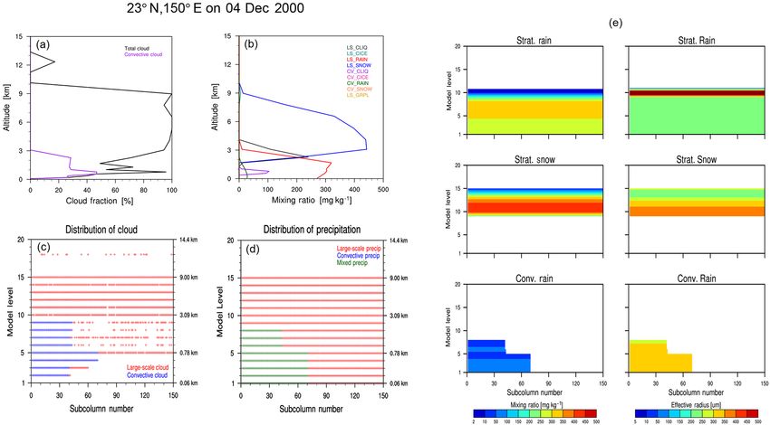
H. Song et al.: Importance of sub-grid cloud variability for model evaluation                                                            3149

Figure 1. (a) PDF of the rainwater mixing ratio for rainwater when the horizontal variability of rainwater is assumed to follow the exponential
distribution. The vertical dashed blue line indicates the mean value of the rainwater mixing ratio as 0.03 g kg−1 . (b) The corresponding PDF
of the CloudSat radar reflectivity simulated by COSP assuming the Marshall and Palmer particle size distribution. The dashed blue line
corresponds to the radar reflectivity based on the mean rainwater 0.03 g kg−1 , and the solid red line corresponds to the grid-mean radar
reflectivity based on the PDF of the rainwater mixing ratio.

In the SPCAM5 COSP run, the sub-grid cloud and precip-                    the model winds are nudged toward the Modern Era Reanaly-
itation properties from the embedded CRMs of SPCAM5                       sis for Research Applications (MERRA) reanalysis with a re-
are used to drive the COSP simulation. In the SPCAM5-                     laxation timescale of 6 h (Zhang et al., 2014). The SPCAM5
Homogeneous COSP run, the default homogenous hydrom-                      simulations are performed from September 2008 to Decem-
eteor scheme of COSP mentioned above is used to generate                  ber 2010 (28 months). The last 24 months’ (January 2009–
the sub-grid cloud and precipitation fields for the COSP sim-             December 2010) outputs of the simulations are used for anal-
ulation. The outputs from the two runs are compared with the              ysis.
collocated CloudSat and MODIS observations to assess the
potential problems in both runs, and also to understand the               2.2   COSP
impacts of omitting sub-grid cloud variations in the COSP
simulations.                                                              We used COSP Version 1.4, which has no scientific dif-
   The rest of the paper is organized as follows: Sect. 2 de-             ference from the latest version, COSP2 (Swales et al.,
scribes the model, COSP, and satellite data used in this study.           2018). Currently, COSP provides simulations of ISCCP (In-
Results are represented in Sect. 3. Finally, Sect. 4 provides             ternational Satellite Cloud Climatology Project), CALIPSO
general conclusions and remarks.                                          (Cloud-Aerosol Lidar and Infrared Pathfinder Satellite Ob-
                                                                          servation), CloudSat, MODIS, and MISR (Multi-angle Imag-
                                                                          ing SpectroRadiometer) cloud measurements and/or re-
2     Description of model, COSP, and satellite                           trievals (Bodas-Salcedo et al., 2011). In this study, we will
      observations                                                        focus on the MODIS and CloudSat simulators (Pincus et al.,
                                                                          2012; Haynes et al., 2007). COSP has three major parts, each
2.1    Model                                                              controlling a step of the pseudo-retrieval process: (1) the sub-
                                                                          column generator of COSP first distributes the grid-mean
The model used in this study is SPCAM5, an application                    cloud and precipitation properties from GCMs into the so-
of the Multiscale Modeling Framework (MMF) (Randall et                    called sub-columns that are conceptually similar to “pix-
al., 2003; Khairoutdinov et al., 2005, 2008; Tao et al., 2009)            els” in satellite remote sensing; (2) the satellite simulators
to CAM5 (Neale et al., 2010), which uses the finite volume                simulate the direct measurements (e.g., CloudSat radar re-
dynamical core at 1.9◦ latitude × 2.5◦ longitude resolution               flectivity and CALIOP backscatter) and retrieval products
with 30 vertical levels and a 600 s time step. The embedded               (e.g., MODIS cloud optical thickness and effective radius)
2-D CRM in each CAM5 grid cell includes 32 columns at                     for each sub-column using highly simplified radiative trans-
4 km horizontal grid spacing and 28 vertical layers coincid-              fer and retrieval schemes; (3) the aggregation scheme av-
ing with the lowest 28 CAM5 levels. The CRM runs with                     erages the sub-column simulations back to grid level to
a 20 s time step. Details of the SPCAM5 can be found in                   obtain temporal–spatial averages that are comparable with
Wang et al. (2011, 2015). The simulations are run in a “con-              aggregated satellite products (e.g., MODIS level-3 gridded
strained meteorology” configuration (Ma et al., 2013, 2015)               monthly mean products).
to facilitate model evaluation against observations, in which

www.geosci-model-dev.net/11/3147/2018/                                                        Geosci. Model Dev., 11, 3147–3158, 2018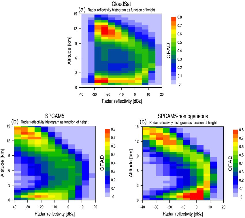
3150                                            H. Song et al.: Importance of sub-grid cloud variability for model evaluation

Figure 2. At the single-grid 23◦ N and 150◦ E on 4 December 2010 in the CAM5-Base simulation (Song et al., 2017): (a) the grid-mean
total (stratiform plus convective) and convective cloud fraction. (b) The grid-mean mixing ratios of cloud and precipitation hydromete-
ors (LS_CLIQ: large-scale (i.e., stratiform) cloud water; LS_CICE: large-scale cloud ice; LS_RAIN: large-scale rain; LS_SNOW: large-
scale snow; LS_GRPL: large-scale graupel; CV_CLIQ: convective cloud water; CV_CICE: convective cloud ice; CV_RAIN: convective
rain; CV_SNOW: convective snow). (c) The distribution of large-scale (red plus signs for frac_out=1) and convective (blue plus signs for
frac_out=2) cloud among the sub-columns generated by the SCOPS scheme (i.e., frac_out from scops.f). (d) The distribution of large-scale
(red plus signs for prec_frac=1), convective (blue plus signs for prec_frac=2), and mixed (green plus signs for prec_frac=3) precipitation
among the sub-columns generated by the SCOPS-PREC scheme (i.e., prec_frac from prec_scops.f). (e) The mixing ratio (left panels) and
effective radius (right panels) of three precipitation hydrometeor types among the sub-columns.

   As mentioned in the Introduction, COSP-v1.4 has a highly               First, sub-columns (150 sub-columns are generated in our
simplified built-in sub-column generator based on the ho-              example) are assigned as either cloudy or clear at each
mogenous hydrometeor scheme. This scheme accounts only                 model level by the Subgrid Cloud Overlap Profile Sampler
for the sub-grid variability of the types of hydrometeors and          (SCOPS), which was developed originally as part of the IS-
ignores the variability of mass and microphysics within each           CCP simulator (Klein and Jakob, 1999; Webb et al., 2001).
hydrometeor type. An example is provided in Fig. 2 to il-              Figure 2c shows the distributions of cloudy sub-columns
lustrate how this default sub-column generator of COSP-                among the 150 sub-columns at each vertical level, indicated
v1.4 distributes the grid-mean cloud and precipitation into            by variable frac_out produced in the scops.f routine. The
the sub-columns. We arbitrarily selected a grid (23◦ N and             sub-column at a certain vertical level is stratiform cloudy if
150◦ E) with both cloud and significant precipitation from             frac_out=1, or connective cloudy if frac_out=2 at that verti-
our previous CAM5 simulation (CAM5-Base simulation in                  cal level. As illustrated in Fig. 2c, the SCOPS assigns cloud
Song et al., 2017). Figure 2a shows the vertical profiles of           to the sub-columns in a manner consistent with the model’s
the grid-mean total (stratiform plus convective) and convec-           grid box average stratiform and convective cloud amounts
tive cloud fractions at the selected grid box. Figure 2b shows         (Fig. 2a) and its cloud overlap assumption, i.e., maximum-
the vertical profiles of the grid-mean mixing ratios of each           random overlap in this case. The next step is to determine
type of hydrometeor. The sub-column generator of COSP                  which of the sub-columns generated by SCOPS contain pre-
takes the grid-mean cloud fractions, hydrometeor mixing ra-            cipitation hydrometeors, e.g., rain and snow. This step is
tios, and effective particle sizes (Fig. 2a and b) as inputs to        necessary and critical for the COSP CloudSat radar simu-
generate the sub-columns for the later satellite measurement           lator (Bodas-Salcedo et al., 2011) because radar reflectiv-
and retrieval simulation.                                              ity is highly sensitive to the precipitation hydrometeors due

Geosci. Model Dev., 11, 3147–3158, 2018                                                   www.geosci-model-dev.net/11/3147/2018/
H. Song et al.: Importance of sub-grid cloud variability for model evaluation 3151
to their large particle size (L’Ecuyer and Stephens, 2002; particles (i.e., 2B-GEOPROF product), from which other in-
Tanelli et al., 2008). The current sub-grid precipitation distri- formation such as vertical distribution of clouds and precip-
bution scheme, “SCOPS-PREC”, is developed and described itation can be derived. The CloudSat 2B-GEOPROF prod-
in Zhang et al. (2010). Figure 2d shows the masking of pre- uct (Marchand et al., 2008) is used for cloud vertical struc-
cipitation among the 150 sub-columns generated by SCOPS- ture, radar reflectivity, and identification of precipitation in
PREC for the example grid. After the cloud and precipitation MBL clouds. To prepare for the comparison of joint statistics,
are masked, the last step is to specify the mass (i.e., mixing we collocated 5 years (2006–2010) of pixel-level (i.e., level-
ratio) and effective radius of hydrometeors for all the sub- 2) MODIS and CloudSat observations using the collocation
columns occupied by clouds and/or precipitation. The cur- scheme developed in Cho et al. (2008). Due to the low sam-
rent scheme for this step is highly simplified. As shown in pling rate of CloudSat, we used 5 years (2006–2010) of ob-
Fig. 2e, it assumes the mass and the microphysics of each servations, in comparison with the 2-year model simulation
type of hydrometeor to be horizontally homogeneous among (2009–2010), to obtain enough statistics. A sensitivity study
all the sub-columns that are occupied by this type of hydrom- indicates that the inter-annual variability of MBL clouds is
eteor at a given model level. In other words, at each model much smaller than the model-to-observation differences.
level the only difference among sub-columns is that they may In this study, we focus on the tropical and subtropical re-
be occupied by different types of hydrometeors (Zhang et al., gions between 45◦ S and 45◦ N (loosely referred to as “trop-
2010). ical and subtropical region”), where most stratocumulus and
In this study, we have carried out two COSP simula- cumulus regimes are found. We avoid high latitudes because
tions using the 2-year SPCAM5 CRM outputs to investi- satellite observations, namely MODIS, may have large un-
gate the importance of considering the sub-grid variations certainties at low solar zenith angles there (Kato and Mar-
of cloud and precipitation properties when evaluating the shak, 2009; Grosvenor and Wood, 2014; Cho et al., 2015).
GCM simulations using COSP. The two COSP simulations
are marked as SPCAM5 COSP and SPCAM5-Homogeneous
COSP, respectively. For the SPCAM5 COSP simulation, we 3 Sensitivity study: SPCAM5 COSP vs.
treat the sub-grid cloud and precipitation fields from the SPCAM5-Homogeneous COSP
CRM of SPCAM5 outputs as sub-columns of COSP without
using the COSP sub-column generator. For the SPCAM5- First, we compare the Contoured Frequency by Altitude
Homogeneous COSP simulation, we first average the sub- Diagram (CFAD) of tropical clouds derived based on SP-
grid cloud and precipitation fields (including both clear and CAM5 COSP and SPCAM5-Homogeneous COSP simula-
cloudy sub-grids) from the CRM of SPCAM5 to each CAM5 tions with that derived from the CloudSat 2B-GEOPROF
grid, and then input these grid-mean cloud and precipitation product in Fig. 3. The CFAD-based CloudSat observations
fields to the default COSP-v1.4 sub-column simulator de- display a typical boomerang-type shape that has been re-
scribed above to generate the sub-column fields. All the other ported in many previous studies (Bodas-Salcedo et al., 2011;
processes of two COSP simulations are exactly the same. The Zhang et al., 2010; Marchand et al., 2009). Focusing on the
COSP simulator outputs are produced from 6-hourly calcu- low clouds below 3 km, we observe a rather broad distribu-
lations and the number of sub-columns used here is 32. To tion of radar reflectivity with a maximum occurrence fre-
derive the probability of precipitation, we made some simple quency around −30 to −20 dBZ followed by a long tail ex-
in-house modifications in COSP v1.4 to write out the MODIS tending to about 10 dBZ. As pointed out in previous studies,
and CloudSat simulations for every sub-column. This allows the peak around −30 to −20 dBZ is due to non-precipitating
us to derive the joint statistics of COSP-MODIS and COSP- MBL clouds and the precipitating clouds with increasing
CloudSat simulations and compare them with those derived rain rate give rise to the long tail. The CFAD based on two
from collocated MODIS and CloudSat level-2 products. COSP simulations exhibits some characteristics similar to
the CloudSat observations, but also many noticeable differ-
2.3 Satellite data ences. In particular, the two COSP simulations both pro-
duce a much narrower range of radar reflectivity for low
The cloud measurements from the A-Train satellite sen- clouds, with occurrence frequency clustered mostly around
sors, namely MODIS and CloudSat, are used for model- −25 dBZ in SPCAM5 COSP and around 0 dBZ in SPCAM5-
to-observation comparison. The newly released collection 6 Homogeneous COSP. These results show that using the over-
(C6) Aqua-MODIS cloud products (Platnick et al., 2017) simplified COSP sub-column generator (e.g., the homoge-
are used to evaluate cloud fraction, cloud optical thickness, neous hydrometeor scheme) has non-negligible influences on
and cloud droplet effective radius. For MBL cloud studies, the simulated radar reflectivity and produces artificially high
CloudSat provides valuable information on the warm rain occurrences of large radar reflectivity. Consistent with many
process that cannot be achieved by a passive sensor like previous studies (e.g., Bodas-Salcedo et al., 2008; Stephens
MODIS. The direct measurement of CloudSat is the vertical et al., 2012; Nam and Quaas, 2012; Franklin et al., 2013; Jing
profile of 94 GHz radar reflectivity by cloud and hydrometer et al., 2017), our results also reveal that GCMs tend to pro-
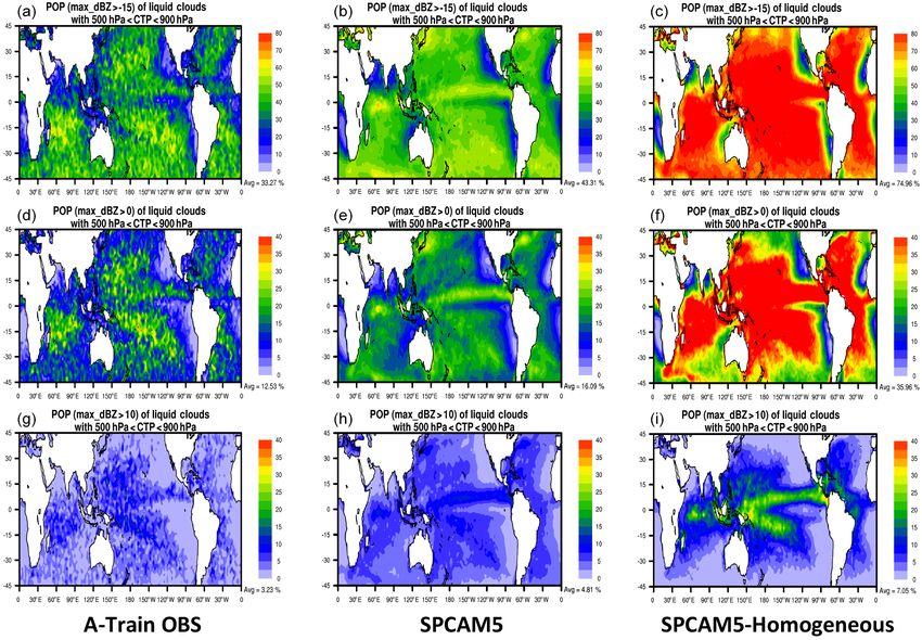
www.geosci-model-dev.net/11/3147/2018/ Geosci. Model Dev., 11, 3147–3158, 20183152 H. Song et al.: Importance of sub-grid cloud variability for model evaluation Figure 3. Tropical-averaged radar reflectivity–height histogram in the CloudSat observation (a), the SPCAM5 CloudSat simulation (b), and the SPCAM5-Homogeneous CloudSat simulation (c). duce much larger radar reflectivity more frequently through served by CloudSat. These clouds are either too thin and the COSP simulator compared to the satellite observation. therefore their radar reflectivity is too weak to be detected The systematic biases in simulated radar reflectivity by the by CloudSat, or they are too low and therefore suffer from COSP homogeneous hydrometeor scheme might lead to the the surface clutter issue (Marchand et al., 2008). For those unjustified and biased evaluation of the warm rain produc- warm liquid clouds detected by both MODIS and Cloud- tion in GCMs, since cloud column maximum radar reflec- Sat, the PDF of Zmax peaks around −25 dBZ. Second, in tivity (Zmax ) is often used to distinguish precipitating from both COSP simulations, almost all warm liquid clouds de- non-precipitating MBL clouds (Kubar and Hartmann, 2009; rived by the MODIS simulator have a valid CloudSat radar Lebsock and Su, 2014; Haynes et al., 2009). reflectivity larger than −40 dBZ. The PDFs of Zmax in SP- Next we compare the simulated and observed probability CAM5 reasonably resemble those in the A-Train observa- density functions (PDFs) of Zmax for all the sub-columns tions. However, significantly different from the other two, the that are marked as warm liquid clouds in the domain be- distribution of Zmax in SPCAM5-Homogeneous shifts to the tween 45◦ S and 45◦ N. The warm liquid clouds are defined large dBZ values and peaks around 0 dBZ. In previous stud- by the cloud phase and cloud top pressure derived from the ies (e.g., Takahashi et al., 2017), warm liquid clouds are cate- MODIS simulator by the criteria that cloud phase is liq- gorized into three different modes by Zmax : non-precipitating uid and cloud top pressure is between 900 and 500 hPa. mode (Zmax < −15 dBZ), drizzle mode (−15 dBZ < Zmax < Big differences in the PDFs of Zmax between the SPCAM5- 0 dBZ), and rain mode (Zmax > 0 dBZ). The simulated and Homogeneous COSP and the A-Train observations, and be- observed PDFs of Zmax demonstrate that a large portion tween SPCAM5-Homogeneous COSP and SPCAM5 COSP, of warm liquid clouds is non-precipitating in the observa- are shown in Fig. 4. First, in the A-Train observations, about tions and SPCAM5 COSP, while most warm liquid clouds 46 % of warm liquid clouds detected by MODIS are not ob- are precipitating (drizzle or rain) clouds in the SPCAM5- Geosci. Model Dev., 11, 3147–3158, 2018 www.geosci-model-dev.net/11/3147/2018/
H. Song et al.: Importance of sub-grid cloud variability for model evaluation 3153
than a certain threshold with respect to the total number of
liquid-phase clouds identified by COSP-MODIS. As shown
in Fig. 5, two COSP simulations show dramatically different
spatial distributions of POPs. The SPCAM5 COSP produces
the similar POP patterns to those in the observations, with the
domain-averaged POPs for drizzle or rain, rain, and heavy
rain being about 43 %, 16 %, and 4.5 %, respectively. How-
ever, the POPs in the SPCAM5-Homogeneous COSP are
substantially overestimated, with the domain-averaged POPs
for drizzle or rain, rain, and heavy rain being about 75 %,
36 %, and 7 %, respectively. Using the COSP homogeneous
hydrometeor scheme will lead to the conclusion that the driz-
zle or rain is triggered too frequently (more than double the
observations) in the SPCAM5 model, which obviously is not
Figure 4. The histograms of column maximum radar reflectiv- a fair assessment.
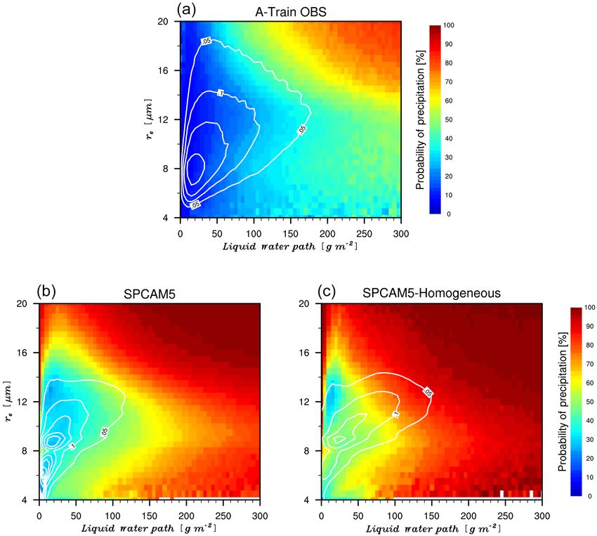
ity for liquid clouds over oceanic regions from 45◦ S to 45◦ N Previous studies find that the warm rain production in
in A-Train satellite observations, SPCAM5 COSP, and SPCAM5- MBL clouds is tightly related to the in-cloud microphys-
Homogeneous COSP simulations. ical properties of MBL clouds (e.g., Stevens et al., 2005;
Wood, 2005; Comstock et al., 2005). Next, we check the de-
pendence of POP on in-cloud properties’ liquid water path
Homogeneous COSP. The use of the COSP homogeneous (LWP) and on liquid cloud effective radius (re ) in both ob-
hydrometeor scheme gives us a dramatically different assess- servations and two COSP simulations. Figure 6 shows the
ment of the warm rain production of MBL clouds in the SP- POPs of drizzle or rain (i.e., Zmax > −15 dBZ) as a func-
CAM5 model; i.e., if we consider the sub-column variability tion of in-cloud LWP and re overlaid by the joint PDF of
of cloud and precipitation in the COSP simulation, we find LWP and re (white contours) in the satellite observations
that the SPCAM5 model can reproduce the observed warm and two COSP simulations. The observed POPs of warm liq-
rain production quite well. However, if we ignore the CRM uid clouds increase monotonically with increasing in-cloud
sub-grid variability and use the homogeneous hydrometeor LWP and re , with high POPs concentrating on the domain
scheme, we may make the biased conclusion that the SP- with large values of LWP and re (i.e., LWP > 200 g m−2 and
CAM5 model performs badly in the simulation of warm rain re > 15 µm). However, in the two COSP simulations, espe-
production. cially the SPCAM5-Homogeneous COSP, at each joint bin
More significant differences between the SPCAM5 COSP the POPs are much larger than those in the A-Train obser-
and SPCAM5-Homogeneous COSP simulations can be vations. When in-cloud LWP (re ) is larger than 150 g m−2
found from the spatial distributions of the probability of pre- (17 µm), the dependence of POPs on in-cloud re (LWP) is
cipitation (POP) in MBL warm clouds (Fig. 5). Here, the small. The joint PDFs of in-cloud LWP and re in the ob-
POP for a given grid box is defined as the fraction of liquid- servations and two COSP simulations are also quite differ-
phase cloud identified by MODIS observations with Zmax ent. There are more occurrences with large LWP and re in
larger than a certain threshold (i.e., −15 dBZ for drizzle or the MODIS observations than the two COSP simulations.
rain, 0 dBZ for rain, and 10 dBZ for heavy rain, respectively) The SPCAM5 COSP simulations have two peaks of the
according to the collocated CloudSat observations with re- joint PDFs, which are converted to one occurrence peak in
spect to the total population liquid-phase clouds with the the SPCAM5-Homogeneous COSP simulation by using the
cloud top pressure between 500 and 900 hPa in the grid. Ob- COSP homogeneous hydrometeor scheme.
servations in Fig. 5 suggest that roughly a third of MBL Based on the above comparisons, we can see that the over-
clouds observed by MODIS in the tropical and subtropi- simplified COSP sub-column generator contributes to not
cal region are likely precipitating (drizzle or rain), with a only the narrow distribution of MBL cloud radar reflectivity,
domain-averaged POP around 33 %. The POP of drizzle plus but also to unrealistically high POPs in the SPCAM5 model.
rain has a distinct pattern: smaller (∼ 15 %) in the coastal Sc Besides, it also changes the distribution of in-cloud micro-
regions and increasing to ∼ 50 % in the Cu cloud regions. physical properties, and the relationship between POPs and
The observed POPs of rain and heavy rain show similar spa- cloud microphysical properties as well.
tial patterns to those of drizzle plus rain, with much smaller
domain-averaged POP being about 12.5 % and 3.3 %, respec-
tively. 4 Summary and discussion
In the same way as we define POP for observations, we
define the POP for two COSP simulations as the ratio of sub- This study presents a satellite-based evaluation of the warm
columns that have COSP-CloudSat simulated Zmax larger rain production of MBL cloud in the SPCAM5 model us-
www.geosci-model-dev.net/11/3147/2018/ Geosci. Model Dev., 11, 3147–3158, 20183154 H. Song et al.: Importance of sub-grid cloud variability for model evaluation Figure 5. Probability of precipitation (POP) of liquid clouds between 500 and 900 hPa levels in the satellite observations (a, d, g), the SPCAM5 COSP simulation (b, e, h), and the SPCAM5-Homogeneous COSP simulation (c, f, i). Three categories of precipitation: drizzle plus rain (column Zmax > −15 dBZ, a, b, c), rain (column Zmax > 0 dBZ, d, e, f), and strong rain only (column Zmax > 10 dBZ, g, h, i). Unit of POP is %. ing two COSP simulations (SPCAM5 COSP and SPCAM5- The systematic and significant biases due to the limitation Homogeneous COSP), with the objective of demonstrating of the current homogeneous hydrometeor scheme can mis- the importance of considering the sub-grid variability of lead the evaluation of GCMs and should not be overlooked. cloud and precipitation when using COSP to evaluate GCM In this regard, an improved sub-column generator needs to simulations. Through the SPCAM5 COSP simulations, in be developed for COSP to account for the sub-grid variances which the sub-column variability of cloud and precipitation of cloud and/or hydrometer mass and microphysics. A recent is considered, we find that the SPCAM5 model can repro- study of Hillman et al. (2018) investigated the sensitivities duce the observed warm rain production quite well. However, of simulated satellite retrievals to subgrid-scale overlap and in the SPCAM5-Homogeneous COSP simulation, in which condensate heterogeneity, and demonstrated the systematic we ignore the CRM sub-grid variability and use the COSP biases in the simulated MODIS cloud fraction and CloudSat homogeneous hydrometeor scheme, the simulated radar re- radar reflectivity due to the oversimplified COSP sub-column flectivity and POPs in the SPCAM5 are significantly overes- generator. Their study also proposed a new scheme to replace timated compared to the observations. Therefore, use of the the COSP current sub-column generator, and showed that COSP homogeneous hydrometeor scheme gives us a signifi- the new scheme can produce much better satellite retrievals. cantly different assessment of warm rain production of MBL Implementing their sub-column heterogeneous hydrometeor clouds in the SPCAM5 model. Our results also indicate that scheme in COSP may improve the GCM COSP simulations the sub-grid variability of mass and microphysics of each hy- and give a better-justified assessment of the GCM perfor- drometeor type is key to the realistic simulation of radar re- mance in simulating warm rain processes and cloud micro- flectivity. physical properties. Geosci. Model Dev., 11, 3147–3158, 2018 www.geosci-model-dev.net/11/3147/2018/
H. Song et al.: Importance of sub-grid cloud variability for model evaluation                                                         3155

Figure 6. POP (drizzle or rain) of liquid clouds at each LWP and liquid cloud effective radius in the satellite observations (a), the SPCAM5
COSP simulation (b), and the SPCAM5-Homogeneous COSP simulation (c). The white solid contours are joint PDF of LWP and liquid
cloud effective radius. Units of POP and PDF are %.

   On the other hand, since the assumptions of sub-grid vari-           development_releases/spcam2_0-cesm1_1_1, last access: 19 July
ability of cloud and hydrometeors in different GCMs may                 2018, registration required). Codes of COSP V1.4 can be found
be quite different, one universal sub-column hydrometeor                on the website at https://github.com/CFMIP/COSPv1 (last access:
scheme may be not applicable to all models. Based on this               19 July 2018). We used the collection 6 (C6) Aqua-MODIS
consideration, the latest version, COSP version 2, enhances             cloud products (Platnick et al., 2017), which can be down-
                                                                        loaded from the NASA website at https://lance3.modaps.eosdis.
flexibility by allowing for model-specific representation of
                                                                        nasa.gov/data_products/ (last access: 19 July 2018). The Cloud-
sub-grid-scale cloudiness and hydrometeor condensates and               Sat data are distributed by the CloudSat Data Processing Cen-
encourages the users to implement the same sub-grid scheme              ter. The CloudSat 2B-GEOPROF product we used is down-
as the host GCM for consistency (Swales et al., 2018). Never-           loaded from the website at http://www.cloudsat.cira.colostate.edu/
theless, our study also suggests that any evaluation study of           data-products/level-2b/2b-geoprof?term=42 (last access: 19 July
warm rain production in GCMs by using COSP simulators                   2018).
should take this issue into account.

                                                                        Author contributions. MW provided the source code of SPCAM5
Code and data availability. Details of SPCAM5 can be found              and wrote the Fortran code to run COSP simulation with the sub-
in Wang et al. (2011, 2015). The host GCM in SPCAM5 is                  grid cloud and precipitation properties from the embedded CRMs of
the Community Atmospheric Model, version 5 (see details on              SPCAM5. PLM and SG provided the results of CAM5 simulations
the CESM website at http://www.cesm.ucar.edu/models/cesm1.1/            and helped us to find the excessive drizzle production problem in
cam/, last access: 19 July 2018). SPCAM5 has recently been              CAM5, which is partially due to the COSP’s over-simplified sub-
merged with CESM1.1.1 and released to the public (Ran-                  column generator. HS and ZZ carried out the SPCAM5 simulation,
dall et al., 2013; https://svn-ccsm-release.cgd.ucar.edu/model_

www.geosci-model-dev.net/11/3147/2018/                                                      Geosci. Model Dev., 11, 3147–3158, 2018
3156 H. Song et al.: Importance of sub-grid cloud variability for model evaluation
drafted the text and made the figures. All authors contributed to the Cho, H. M., Yang, P., Kattawar, G. W., Nasiri, S. L., Hu, Y., Minnis,
editing of the manuscript. P., Trepte, C., and Winker, D.: Depolarization ratio and attenu-
ated backscatter for nine cloud types: Analyses based on collo-
cated CALIPSO lidar and MODIS measurements, Opt. Express,
Competing interests. The authors declare that they have no conflict 16, 3931–3948, 2008.
of interest. Cho, H. M., Zhang, Z., Meyer, K., Lebsock, M., Platnick, S.,
Ackerman, A. S., Di Girolano, L., C.-Labonnote, L., Cornet,
C., Riedi, J., and Holz, R. E.: Frequency and causes of failed
Acknowledgements. This research is supported by the U.S. MODIS cloud property retrievals for liquid phase clouds over
Department of Energy (DOE), Office of Science, Biological and global oceans, J. Geophys. Res.-Atmos., 120, 2015JD023161,
Environmental Research, Regional and Global Climate Mode Anal- https://doi.org/10.1002/2015JD023161, 2015.
ysis Program (grant no. DE-SC0014641). The Pacific Northwest Comstock, K. K., Bretherton, C. S., and Yuter, S. E.: Mesoscale
National Laboratory is operated for the DOE by Battelle Memorial variability and drizzle in southeast Pacific stratocumulus, J. At-
Institute under contract DE-AC05-76RLO 1830. Minghuai Wang mos. Sci., 62, 3792–3807, https://doi.org/10.1175/JAS3567.1,
was supported by the Minister of Science and Technology of 2005.
China (2017YFA0604001). The computations in this study were Franklin, C. N., Sun, Z., Bi, D., Dix, M., Yan, H., and
performed at the UMBC High Performance Computing Facility Bodas-Salcedo, A.: Evaluation of clouds in access using
(HPCF). The facility is supported by the U.S. National Science the satellite simulator package COSP: regime-sorted tropical
Foundation through the MRI program (grant nos. CNS-0821258 cloud properties, J. Geophys. Res.-Atmos., 118, 6663–6679,
and CNS-1228778) and the SCREMS program (grant no. DMS- https://doi.org/10.1002/jgrd.50496, 2013.
0821311), with substantial support from UMBC. The MODIS Grosvenor, D. P. and Wood, R.: The effect of solar zenith angle on
cloud products used in this study are downloaded from the NASA MODIS cloud optical and microphysical retrievals within ma-
Level-1 and Atmosphere Archive and Distribution System from rine liquid water clouds, Atmos. Chem. Phys., 14, 7291–7321,
https://ladsweb.modaps.eosdis.nasa.gov/ (last access: 19 July https://doi.org/10.5194/acp-14-7291-2014, 2014.
2018). The CloudSat products are provided by the CloudSat Data Haynes, J. M., Marchand, R. T., Luo, Z., Bodas-Salcedo, A., and
Processing Center from http://www.cloudsat.cira.colostate.edu/ Stephens, G. L.: A multi-purpose radar simulation package:
(last access: 19 July 2018). QuickBeam, B. Am. Meteorol. Soc., 88, 1723–1727, 2007.
Haynes, J. M., L’Ecuyer, T. S., Stephens, G. L., Miller, S. D.,
Edited by: Klaus Gierens Mitrescu, C., Wood, N. B., and Tanelli, S.: Rainfall retrieval
Reviewed by: two anonymous referees over the ocean with spaceborne W-band radar, J. Geophys. Res.-
Atmos., 114, D00A22, https://doi.org/10.1029/2008JD009973,
2009.
Hillman, B. R., Marchand, R. T., and Ackerman, T. P.: Sen-
sitivities of simulated satellite views of clouds to subgrid-
References scale overlap and condensate heterogeneity, J. Geophys. Res.-
Atmos.,https://doi.org/10.1029/2017jd027680, accepted, 2018.
Bodas-Salcedo, A., Webb, M. J., Brooks, M. E., Ringer, M. A., Jing, X., Suzuki, K., Guo, H., Goto, D., Ogura, T., Koshiro,
Williams, K. D., Milton, S. F., and Wilson, D. R.: Evaluating T., and Mülmenstädt, J.: A multimodel study on warm
cloud systems in the Met Office global forecast model using precipitation biases in global models compared to satellite
simulated CloudSat radar reflectivities, J. Geophys. Res., 113, observations, J. Geophys. Res.-Atmos., 122, 11806–11824,
D00A13, https://doi.org/10.1029/2007JD009620, 2008. https://doi.org/10.1002/2017JD027310, 2017.
Bodas-Salcedo, A., Webb, M. J., Bony, S., Chepfer, H., Dufresne, Kato, S. and Marshak, A.: Solar zenith and viewing geome-
J.-L., Klein, S. A., Zhang, Y., Marchand, R., Haynes, J. M., Pin- try dependent errors in satellite retrieved cloud optical thick-
cus, R., and John, V. O.: COSP: Satellite simulation software ness: Marine Sccase, J. Geophys. Res.-Atmos., 114, D01202,
for model assessment, B. Am. Meteorol. Soc., 92, 1023–1043, https://doi.org/10.1029/2008JD010579, 2009.
https://doi.org/10.1175/2011BAMS2856.1, 2011. Kay, J. E., Hillman, B. R., Klein, S. A., Zhang, Y., Medeiros, B.,
Bony, S. and Dufresne, J.-L.: Marine boundary layer clouds Pincus, R., Gettelman, A., Eaton, B., Boyle, J., Marchand, R.,
at the heart of tropical cloud feedback uncertainties and Ackerman, T. P.: Exposing global cloud biases in the com-
in climate models, Geophys. Res. Lett., 32, L20806, munity atmosphere model (CAM) using satellite observations
https://doi.org/10.1029/2005GL023851, 2005. and their corresponding instrument simulators, J. Climate, 25,
Cess, R., Zhang, M. H., Ingram, W. J., Potter, G. L., Alekseev, V., 5190–5207, https://doi.org/10.1175/JCLI-D-11-00469.1, 2012.
Barker, H. W., Cohen-Solal, E., Colman, R. A., Dazlich, D. A., Kay, J. E., L’Ecuyer, T., Chepfer, H., Loeb, N., Morrison, A., and
Del Genio, A. D., Dix, M. R., Dymnikov, V., Esch, M., Fowler, Cesana, G.: Recent Advances in Arctic Cloud and Climate Re-
L. D., Fraser, J. R., Galin, V., Gates, W. L., Hack, J. J., Kiehl, search, Current Climate Change Reports, 2, 159–169, 2016.
J. T., Le Treut, H., Lo, K. K.-W., McAvaney, B. J., Meleshko, Khairoutdinov, M. F. and Randall, D. A.: Cloud resolving modeling
V. P., Morcrette, J.-J., Randall, D. A., Roeckner, E., Royer, J.-F., of the ARM summer 1997 IOP: Model formulation, results, un-
Schlesinger, M. E., Sporyshev, P. V., Timbal, B., Volodin, E. M., certainties, and sensitivities, J. Atmos. Sci., 60, 607–625, 2003.
Taylor, K. E., Wang, W., and Wetherald, R. T.: Cloud feedback in Khairoutdinov, M., Randall, D., and DeMott, C.: Simulations of the
atmospheric general circulation models: An update, J. Geophys. atmospheric general circulation using a cloud-resolving model
Res.-Atmos., 101, 12791–12794, 1996.
Geosci. Model Dev., 11, 3147–3158, 2018 www.geosci-model-dev.net/11/3147/2018/H. Song et al.: Importance of sub-grid cloud variability for model evaluation 3157
as a superparameterization of physical processes, J. Atmos. Sci., Pincus, R., Platnick, S., Ackerman, S. A., Hemler, R. S., and Hof-
62, 2136–2154, 2005. mann, P.: Reconciling simulated and observed views of clouds:
Klein, S. A. and Jakob, C.: Validation and sensitivities of MODIS, ISCCP, and the limits of instrument simulators, J.
frontal clouds simulated by the ECWMF model, Mon. Climate, 25, 120220120058001, https://doi.org/10.1175/JCLI-
Weather Rev., 127, 2514–2531, https://doi.org/10.1175/1520- D-11-00267.1, 2012.
0493(1999)1272.0.CO;2, 1999. Platnick, S., Meyer, K. G., King, M. D., Wind, G., Amarasinghe, N.,
Kubar, T. L. and Hartmann, D. L.: Understanding the importance Marchant, B., Arnold, G. T., Zhang, Z., Hubanks, P. A., Holz, R.
of microphysics and macrophysics for warm rain in marine low E., Yang, P., Ridgway, W. L., and Riedi, J.: The MODIS cloud
clouds. Part I: Satellite observations, J. Atmos. Sci., 66, 2953– optical and microphysical products: Collection 6 updates and ex-
2972, https://doi.org/10.1175/2009JAS3071.1, 2009. amples from Terra and Aqua, IEEE T. Geosci. Remote, 55, 502–
Lebsock, M. and Su, H.: Application of active spaceborne remote 525, https://doi.org/10.1109/TGRS.2016.2610522, 2017.
sensing for understanding biases between passive cloud wa- Randall, D., Khairoutdinov, M., Arakawa, A., and Grabowski, W.:
ter path retrievals, J. Geophys. Res.-Atmos., 119, 8962–8979, Breaking the cloud parameterization deadlock, B. Am. Meteorol.
https://doi.org/10.1002/2014JD021568, 2014. Soc., 84, 1547–1564, 2003.
Lebsock, M., Morrison, H., and Gettelman, A.: Microphysical im- Randall, D., Branson, M., Wang, M., Ghan, S., Craig, C., Gettel-
plications of cloud-precipitation covariance derived from satel- man, A., and Edwards, J.: A community atmosphere model with
lite remote sensing, J. Geophys. Res.-Atmos., 118, 6521–6533, superparameterized clouds, Eos Trans. AGU, 94, 221–222, 2013.
https://doi.org/10.1002/jgrd.50347, 2013. Song, H., Zhang, Z., Ma, P.-L., Ghan, S., and Wang, M.: An Eval-
L’Ecuyer, T. S. and Stephens, G. L.: An estimation-based precipita- uation of Marine Boundary Layer Cloud Property Simulations
tion retrieval algorithm for attenuating radars, J. Appl. Meteorol., in Community Atmosphere Model Using Satellite Observations:
41, 272–285, 2002. Conventional Sub-grid Parameterization vs. CLUBB, J. Climate,
Ma, P.-L., Rasch, P. J., Wang, H., Zhang, K., and Easter, R. 31, 2299–2320, 2018.
C.: The role of circulation features on black carbon trans- Stephens, G. L., Vane, D. G., Boain, R. J., Mace, G. G., Sassen,
port into the Arctic in the Community Atmosphere Model ver- K., Wang, Z., Illingworth, A. J., O’connor, E. J., Rossow, W.
sion 5 (CAM5), J. Geophys. Res.-Atmos., 118, 4657–4669, B., Durden, S. L., Miller, S. D., Austin, R. T., Bendetti, A.,
https://doi.org/10.1002/jgrd.50411, 2013. Mitrescu, C., and the CloudSat Science Team: The CloudSat
Ma, P.-L., Rasch, P. J., Wang, M., Wang, H., Ghan, S. J., Mission and the A-Train, B. Am. Meteorol. Soc., 83, 1771–1790,
Easter, R. C., Gustafson Jr., W. I., Liu, X., Zhang, Y., https://doi.org/10.1175/BAMS-83-12-1771, 2012.
and Ma, H.-Y.: How does increasing horizontal resolution in Stevens, B., Vali, G., Comstock, K., Woods, R., Van Zanten, M. C.,
a global climate model improve the simulation of aerosol- Austin, P. H., Bretherton, C. S., and Lenschow, D. H.: Pockets of
cloud interactions?, Geophys. Res. Lett., 42, 5058–5065, open cells and drizzle in marine stratocumulus, B. Am. Meteorol.
https://doi.org/10.1002/2015GL064183, 2015. Soc., 86, 51–57, 2005.
Marchand, R., Mace, G. G., Ackerman, T., and Stephens, G.: Suzuki, K., Stephens, G., Bodas-Salcedo, A., Wang, M., Golaz, J.-
Hydrometeor detection using Cloudsat – An earth-orbiting 94- C., Yokohata, T., and Koshiro, T.: Evaluation of the warm rain
GHz cloud radar, J. Atmos. Ocean. Technol., 25, 519–533, formation process in global models with satellite observations, J.
https://doi.org/10.1175/2007JTECHA1006.1, 2008. Atmos. Sci., 72, 3996–4014, https://doi.org/10.1175/JAS-D-14-
Marchand, R., Haynes, J., Mace, G. G., Ackerman, T., and 0265.1, 2015.
Stephens, G.: A comparison of simulated cloud radar output from Swales, D. J., Pincus, R., and Bodas-Salcedo, A.: The Cloud
the multiscale modeling framework global climate model with Feedback Model Intercomparison Project Observational Sim-
CloudSat cloud radar observations, J. Geophys. Res.-Atmos., ulator Package: Version 2, Geosci. Model Dev., 11, 77–81,
114, D00A20, https://doi.org/10.1029/2008JD009790, 2009. https://doi.org/10.5194/gmd-11-77-2018, 2018.
Morrison, H. and Gettelman, A.: A new two-moment bulk strati- Takahashi, H., Lebsock, M., Suzuki, K., Stephens, G., and Wang,
form cloud microphysics scheme in the community atmosphere M.: An investigation of microphysics and subgrid-scale variabil-
model, version 3 (CAM3). Part I: Description and numerical ity in warm-rain clouds using the A-Train observations and a
tests, J. Climate, 21, 3642–3659, 2008. multiscale modeling framework, J. Geophys. Res.-Atmos., 122,
Morrison, H., Curry, J. A., and Khvorostyanov, V. I.: A new double- 7493–7504, 2017.
moment microphysics parameterization for application in cloud Tanelli, S., Durden, S. L., Im, E., Pak, K. S., Reinke, D. G., Partain,
and climate models. Part I: Description, J. Atmos. Sci., 62, 1665– P., Haynes, J. M., and Marchand, R. T.: CloudSat’s Cloud Pro-
1677, 2005. filing Radar After Two Years in Orbit: Performance, Calibration,
Nam, C. and Quaas, J.: Evaluation of clouds and precipitation and Processing, IEEE T. Geosci. Remote, 46, 3560–3573, 2008.
in the ECHAM5 general circulation model using CALIPSO Tao, W. K., Chern, J., Atlas, R., Randall, D., Lin, X., Khairoutdinov,
and CloudSat satellite data, J. Climate., 25, 4975–4992, M., Li, J.-L., Waliser, D. E., Hou, A., Peters-Lidard, C., Lau, W.,
https://doi.org/10.1175/JCLI-D-11-00347.1, 2012. and Simpson, J.: A multiscale modeling system developments,
Neale, R. B., Collins, W. D., Rasch, P. J., Boville, B. A., Hack, J. J., applications, and critical issues, B. Am. Meteorol. Soc., 90, 515–
McCaa, J. R., Williamson, D. L., Kiehl, J. T., and Briegleb, B.: 534, 2009.
Description of the NCAR community atmosphere model (CAM Wang, M., Ghan, S., Easter, R., Ovchinnikov, M., Liu, X., Kas-
5.0), Tech. Rep. TN–486+STR, 268 pp., Natl. Cent. for Atmos. sianov, E., Qian, Y., Gustafson Jr., W. I., Larson, V. E.,
Res., Boulder, Colo., 2010. Schanen, D. P., Khairoutdinov, M., and Morrison, H.: The
multi-scale aerosol-climate model PNNL-MMF: model de-
www.geosci-model-dev.net/11/3147/2018/ Geosci. Model Dev., 11, 3147–3158, 20183158 H. Song et al.: Importance of sub-grid cloud variability for model evaluation scription and evaluation, Geosci. Model Dev., 4, 137–168, Zhang, K., Wan, H., Liu, X., Ghan, S. J., Kooperman, G. J., Ma, https://doi.org/10.5194/gmd-4-137-2011, 2011. P.-L., Rasch, P. J., Neubauer, D., and Lohmann, U.: Techni- Wang, M., Larson, V., Ghan, S., Ovchinnikov, M., Schanen, D., cal Note: On the use of nudging for aerosol–climate model Xiao, H., Liu, X., Guo, Z., and Rasch, P.: A multiscale mod- intercomparison studies, Atmos. Chem. Phys., 14, 8631–8645, eling framework model (superparameterized CAM5) with a https://doi.org/10.5194/acp-14-8631-2014, 2014. higher-order turbulence closure: Model description and low- Zhang, Y., Klein, S. A., Boyle, J., and Mace, G. G.: Evalu- cloud simulations, J. Adv. Model. Earth Syst., 7, 484–509, ation of tropical cloud and precipitation statistics of Com- https://doi.org/10.1002/2014MS000375, 2015. munity Atmosphere Model version 3 using CloudSat and Webb, M., Senior, C., Bony, S., and Morcrette, J.: Combining ERBE CALIPSO data, J. Geophys. Res.-Atmos., 115, D12205, and ISCCP data to assess clouds in the Hadley Centre, ECMWF https://doi.org/10.1029/2009JD012006, 2010. and LMD atmospheric climate models, Clim. Dynam., 17, 905– 922, 2001. Wood, R.: Drizzle in stratiform boundary layer clouds. Part I: Ver- tical and horizontal structure, J. Atmos. Sci., 62, 3011–3033, 2005. Geosci. Model Dev., 11, 3147–3158, 2018 www.geosci-model-dev.net/11/3147/2018/
You can also read