Performance of offline passive tracer advection in the Regional Ocean Modeling System (ROMS; v3.6, revision 904) - GMD
←
→
Page content transcription
If your browser does not render page correctly, please read the page content below
Geosci. Model Dev., 14, 391–407, 2021
https://doi.org/10.5194/gmd-14-391-2021
© Author(s) 2021. This work is distributed under
the Creative Commons Attribution 4.0 License.

Performance of offline passive tracer advection in the Regional
Ocean Modeling System (ROMS; v3.6, revision 904)
Kristen M. Thyng1 , Daijiro Kobashi1 , Veronica Ruiz-Xomchuk1 , Lixin Qu2 , Xu Chen3 , and Robert D. Hetland1,a
1 Department  of Oceanography, Texas A&M University, College Station, TX, USA
2 Department  of Earth System Science, Stanford University, Stanford, CA, USA
3 Center for Ocean-Atmospheric Prediction Studies, Florida State University, Tallahassee, FL, USA
a now at: Pacific Northwest National Laboratory, Richland, WA, USA

Correspondence: Kristen M. Thyng (kthyng@tamu.edu)

Received: 2 July 2020 – Discussion started: 9 September 2020
Revised: 18 November 2020 – Accepted: 8 December 2020 – Published: 25 January 2021

Abstract. Offline advection schemes allow for low-                   1   Introduction
computational-cost simulations using existing model output.
This study presents the approach and assessment for passive
offline tracer advection within the Regional Ocean Modeling          The ability to integrate Eulerian tracer fields offline or sepa-
System (ROMS). An advantage of running the code within               rate from the online original full simulation is attractive be-
ROMS itself is consistency in the numerics on- and offline.          cause of the improved computational efficiency. Once an on-
We find that the offline tracer model is robust: after about 14 d    line simulation has been run, any number of offline simu-
of simulation (almost 60 units of time normalized by the ad-         lations can be run, forced by the stored online model out-
vection timescale), the skill score comparing offline output         put, using a larger time step, and only needing to inte-
to the online simulation using the TS_U3HADVECTION and               grate the transport field itself. This allows for many sim-
TS_C4VADVECTION (third-order upstream horizontal ad-                 ulations when, in contrast, fewer would have been possi-
vection and fourth-order centered vertical advection) tracer         ble with the online simulation. This study presents the de-
advection schemes is 99.6 % accurate for an offline time step        velopment and assessment of an offline passive tracer ad-
20 times larger than the online time step as well as online out-     vection model that is part of the Regional Ocean Model-
put saved with a period below the advection timescale. For           ing System (ROMS), version 904, in the Coupled Ocean–
the MPDATA tracer advection scheme, accuracy is more vari-           Atmosphere–Wave–Sediment Transport (COAWST) model-
able with the offline time step and forcing input frequency          ing system (Shchepetkin and McWilliams, 2005; Warner
choices, but it is still over 99 % for many reasonable choices.      et al., 2010). While the ultimate goal of this work is to run
Both schemes are conservative. Important factors for main-           ROMS with both offline floats representing oil and tracers
taining high offline accuracy are outputting from the online         representing biological processes, along with sediment–oil
simulation often enough to resolve the advection timescale,          interactions, the present focus is on the offline tracer model
forcing offline using realistic vertical salinity diffusivity val-   with a passive tracer.
ues from the online simulation, and using double precision to           Previous work has been done in this area with other mod-
save results.                                                        els. An offline tracer model for the Massachusetts Institute
                                                                     of Technology (MIT) general circulation model (MITgcm)
                                                                     was developed and showed good accuracy (Hill et al., 2004).
                                                                     For a set output frequency, an offline time step of 8 times
                                                                     the online time step gave a skill score of over 98 %. An of-
                                                                     fline tracer model based on MITgcm has been used in sev-
                                                                     eral studies (Dutkiewicz et al., 2001; McKinley et al., 2004).
                                                                     Another offline tracer model, the offline global 3D ocean

Published by Copernicus Publications on behalf of the European Geosciences Union.
392                                           K. M. Thyng et al.: Performance of offline passive tracer advection in ROMS

tracer model (OFFTRAC), is based on the Hallberg Isopy-
cnal Model (HIM) and has been used for long-term biogeo-
chemical integration (Zhang et al., 2014). Other tracer mod-
els have been developed separately from a full numerical
ocean simulator. Gillibrand and Herzfeld (2016) developed a
separate tracer advection model that is not numerically lim-
ited by the Courant number as is expected in the present case.
Another such model developed by Khatiwala et al. (2005) has
a different approach entirely to offline tracer advection, us-
ing a mathematical approach that is distinct from more com-
monly used numerical tracer integration. Interestingly, Lévy
et al. (2012) found that for particular dynamical scenarios,
degrading online model output spatially can result in offline
computational savings with little accuracy degradation.
   The offline tracer model described in this paper is inte-       Figure 1. Model domain and initial blob of passive dye at the sur-
grated into and derived from the ROMS model: preprocessor          face for the first set of numerical experiments.
flag choices allow access to the offline capability. While not
being derived from a specific ocean model allows for wider
potential use, as in some of the previously described models,
there may be an advantage in using the offline model that is       tions (Fox et al., 2002; Cummings, 2005; Chassignet et al.,
a derivative of the offline model to ensure consistency, us-       2007; Cummings and Smedstad, 2013). The surface forcing
ing the exact same numerics and setup. The expected user           is provided by hourly Climate Forecast System Reanalysis
for this software is someone who uses ROMS for their ocean         (CFSR) data (Saha et al., 2010), and air–sea turbulent fluxes
modeling needs and wants to have the ability to run more           are calculated using bulk formula COARE 3.0 (Fairall et al.,
tracer simulations, decoupled from their more expensive on-        2003). In order to realistically simulate the water properties
line simulations. Another type of user may simply have some        and dynamics in the coastal area, 21 daily river discharges
ROMS output available, and this code will allow them to            with specified water transport flux and temperature (from the
leverage it beyond its originally intended use.                    United States Geological Survey) are implemented as bound-
   The experimental setup is described in Sect. 2; this in-        ary fluxes along the coast. To stabilize the open boundaries,
cludes a description of the model setup (Sect. 2.1), the offline   lateral nudging layers are set at the open ocean boundaries.
experiments (Sect. 2.2), and the metrics used for evaluation       The nudging timescale is 0.04 d at the boundary and is grad-
(Sect. 2.3). Results are shown in Sect. 3, and a discussion        ually tuned to 10 d at the 18th interior grid. The climatology
of results is given in Sect. 4. Specific code descriptions are     used for the nudging process is also provided by the HY-
provided in the Appendix: code changes made for robust of-         COM output. This online model ran for 90 d, from 20 April
fline tracer advection (Appendix B) and a description of how       to 19 July 2010, but a subset of 14 d is used for the present
to set up both online and offline simulations for best results     experiments.
(Appendix C).
                                                                   2.2     Offline experiments

2     Experimental setup                                           2.2.1    Full water column Gaussian

2.1    Online model setup                                          A series of online and offline simulations were run to evalu-
                                                                   ate the comparative performance of offline tracer advection.
The online model is set up for the northern Gulf of Mex-           The first set of numerical experiments presented in this paper
ico (25.6–30.6◦ N, 94–84◦ W). The domain was chosen be-            were initialized with a discrete Gaussian blob of dye south-
cause the final goal of this work is to simulate the fate of       west of the Mississippi River delta in a regional model of
oil spilled in this region in 2010. The horizontal resolution      the northern Gulf of Mexico (see Fig. 1). The blob of dye
is 0.04◦ to fully resolve mesoscale processes, and there are       extended fully through the water column. Online simula-
50 vertical layers with refinement at the seabed and sea sur-      tions were run with two tracer advection schemes: MPDATA
face (the transformation equation parameter Vstretching            (both horizontal and vertical), and TS_U3HADVECTION
is 5, and the stretching function parameter Vtransform             and TS_C4VADVECTION (third-order upstream horizontal
is 2) (Azevedo Correia de Souza et al., 2015). The time            advection and fourth-order centered vertical advection, re-
step is 20 s. Hybrid Coordinate Ocean Model (HYCOM)                spectively, which is shortened to U3C4 for the remainder of
Global Reanalysis data (experiment “GLBu0.08/expt_19.1”)           the paper). Additionally, the online simulations were output
are used to initialize the model and provide boundary condi-       at different frequencies, as multiples of the time step (the

Geosci. Model Dev., 14, 391–407, 2021                                                https://doi.org/10.5194/gmd-14-391-2021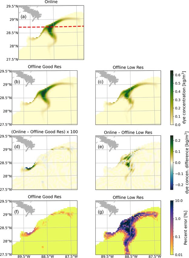
K. M. Thyng et al.: Performance of offline passive tracer advection in ROMS                                                          393

nhis and navg parameters for ROMS):

nhis = 1, 2, 5, 10, 20, 50, 100, 200, 500, 1000, 2000, 5000.

Given that the time step of the online simulation was 20 s,
these correspond to output frequencies of about 20 s, 40 s,
100 s, 3.3 min, 6.7 min, 16.7 min, 0.56 h, 1.1 h, 2.8 h, 5.6 h,
11 h, and 28 h, respectively. Online simulations were saved
as both instantaneous snapshots (his files from ROMS) and
as averages across time steps (avg files from ROMS).
   These offline simulations were run using one of the two
tracer advection schemes, with either his or avg files as
climatology at the output frequency from the online sim-
ulations (controlled by nhis/navg). Additionally, they
were optionally forced by the vertical salinity diffusion vari-
able, Aks, as calculated by the online simulation or by
just the background value. Finally, for an input climatology
file from an online simulation of a given output frequency
(nhis/navg), offline simulations were run with a time step
from the list of nhis values of up to the same output fre-
quency as the online simulation. A time step of 50 times
the online time step was found to lead to unstable solutions;
thus, in effect, the offline time step could be 1, 2, 5, 10, or 20
times the online time step, but it could never be larger than
the nhis value for the given simulation. Also note that the
offline time step needs to divide evenly into the output fre-
quency in the climatology file so that only two time steps are
being accessed at a time. Therefore, for a climatology forcing
file of nhis = 50, the offline simulation could not be forced
with dt = 20.
   The relevant controlling timescale for this simulation is
the advection timescale. Results from online simulations             Figure 2. Second experiment: discrete Gaussian blob of dye at
of the dye advection show a representative length scale of           800 m depth. Subplots show the domain and bathymetry (a), the
about L = 10 km and a speed of about U = 0.5 m s−1 , giv-            dye slice at 800 m depth (b), and the vertical cross section of the
ing an advection timescale of T = L/U = 20 000 s, or about           dye field (c) across the red dashed line in panel (a). The red circle
                                                                     in panel (a) indicates the center of the dye blob.
5.6 h. This timescale is specific to the location of the dye
patch, which is off the continental shelf and responding to
mesoscale processes. If the dye patch was on the shelf, one          resolution” test case, and one with the online output fre-
would expect a shorter timescale. The timescale will be used         quency forced at nhis = 1000 (about 5.5 h) to be used as
to normalize times given in the results and to interpret accu-       a “low-resolution” test case; both were run with the U3C4
racy in relation to offline time choices.                            tracer advection scheme and an offline time step of 20 times
                                                                     the online time step, or 400 s.
2.2.2   At-depth realistic Gaussian
                                                                     2.3     Metrics
Another set of simulations were run to apply the lessons
learned in the first set to a more realistic test case (Fig. 2).     2.3.1    Skill score
This test case is meant to represent an infusion of some ma-
terial to the ocean at depth, for example dissolved methane          The main metric used to evaluate the performance of this
gas. However, as we are testing only the passive offline             model is a skill score, SS (Bogden et al., 1996; Hill et al.,
tracer advection scheme in the present study, the tracer is          2004; Hetland, 2006). This is calculated as follows:
passive and has no particular behavior specific to a mate-                    p
rial. The dye is initialized in a discrete Gaussian blob at                      h(Don − Doff )2 i
800 m depth between 28 and 29◦ N latitude. Building off in-          SS = 1 −       p              ,                          (1)
                                                                                         2 i
                                                                                      hDon
formation from the previous simulations, only two offline
simulations were run: one with the online output frequency           where Doff and Don are the volume of dye on the 3D grid
forced at nhis = 100 (about 30 min) to be used as a “good-           and in time for the off- and online simulations, respectively,

https://doi.org/10.5194/gmd-14-391-2021                                                     Geosci. Model Dev., 14, 391–407, 2021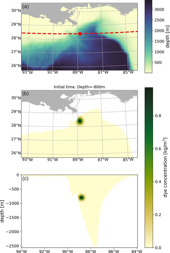
394                                                       K. M. Thyng et al.: Performance of offline passive tracer advection in ROMS

and the brackets h.i indicate averaging over horizontal and                  3     Results
vertical dimensions, returning a time series.
   Often skill scores are calculated with respect to a refer-                3.1    Full water column Gaussian
ence. For example, for numerical model performance, the
difference between model and data in the numerator may                       The accuracy of selected offline simulations is presented
be compared with the difference between climatology and                      here. As there were over 300 offline simulations, only se-
data in the denominator in order to assess how much better                   lected results are shown to best illustrate specific points and
the model is performing than simple climatology (Hetland,                    show the overall performance of the model under a range of
2006). An analogous comparison may be made here vs. per-                     parameter choices. Offline simulations are forced by snap-
sistence of the initial condition of the dye patch, so that this             shots of online output (his, not avg files) in all cases un-
skill score shows how well the offline model performs com-                   less specified. These results are specific to this model setup
pared with simply persisting the initial condition:                          and the dynamics that are being captured in the region, but
                                                                             they should give specific results for other geographically in-
               p                                                             terested users with similar model setups and general guiding
                   h(Doff − Don )2 i                                         results for others.
SSp = 1 − p                                                           (2)
                h(Dinitial − Don )2 i                                           Instantaneous differences in dye concentration demon-
                                                                             strate the spatial structure of the offline simulation errors
                                                                             (Fig. 3). The structure changes not just with changes in the
Skill scores are a comparison between an offline simulation                  frequency of forcing in the offline simulation (nhis) and of-
and the online simulation from which it is forced, unless oth-               fline time step (dt) but also with the tracer advection scheme
erwise noted; thus, the skill score represents the accuracy of               used. Comparing the top two rows in Fig. 3, we see that the
the offline simulation to the online simulation, or the skill in             error in the MPDATA simulations tends to be more localized
faithfully reproducing the online simulation. This is different              when compared with the U3C4 simulations. The magnitude
from a measure of the accuracy of the online simulation itself               of error increases with both a decrease in forcing frequency
to simulate the dynamics.                                                    and an increase in time step for the offline simulations (mov-
                                                                             ing from subplots A to C); in particular, the MPDATA simu-
2.3.2    Percent error                                                       lation shows much more widespread spatial structure in the
                                                                             errors with dt = 20 (subplots C). Subplots E and F show
Percent error is used to demonstrate the accuracy of the sec-                fairly similar structure across the simulations, although with
ond set of simulations in space, because it is not averaged                  larger errors for MPDATA. Subplots D show the much larger
over spatial dimensions like the skill score. The percent error              errors that result when the vertical salinity diffusion coeffi-
at time t0 is calculated as follows:                                         cient Aks is not forced in the offline simulation.
                                                                                Skill scores (Eq. 1) over time, demonstrating offline model
                                                                             accuracy, are shown in Fig. 4, and a summary is shown in Ta-
           |Don (t0 , z, y, x) − Doff (t0 , z, y, x)|                        ble A1. Both tracer advection schemes (U3C4 and MPDATA)
E(t0 ) =                                              ,               (3)
                 Von (t0 , z, y, x)dmax (t0 )                                give highly accurate results (Fig. 4a), though U3C4 performs
                                                                             a bit better than MPDATA. When vertical salinity diffusiv-
                                                                             ity, Aks, which controls the impact of sub-grid-scale vertical
where D* (t0 , z, y, x) is the on- or offline dye volume at time
                                                                             mixing on the tracer field, is not forced (Aksoff), offline ac-
t0 in space (kg), Von (t0 , z, y, x) is the online volume of the
                                                                             curacy is reduced, though just 2 percentage points over 14 d
grid cells (m3 ), and dmax (t0 ) is the maximum dye concentra-
                                                                             compared with when it is forced. The impact of how often
tion at t0 (kg m−3 ). The percent error represents the differ-
                                                                             online model output is saved and input into the offline sim-
ence in the offline from the online simulation compared with
                                                                             ulation, controlled by the nhis parameter, is almost negli-
the maximum possible dye mass at that time step.
                                                                             gible below 200 or 500 times the online time step (nhis
                                                                             200, about 1.1 h, and nhis 500, about 2.8 h, respectively),
2.4     Simulations and software                                             but it has increasing impact for less frequent online model
                                                                             output (higher values of nhis, Fig. 4b). This means that for
Simulations were performed on a Linux cluster with 84 pro-                   the present model setup and region, the frequency of online
cessors for online simulations and 28 processors for offline                 output higher than about 1–3 h is not important. Results are
simulations. The number used was not optimized. Analy-                       relatively similar with nhis 1000 (about 5 h), but accuracy
sis was performed in a Jupyter notebook (Kluyver et al.,                     decreases significantly as nhis increases beyond that. Con-
2016) using pandas (McKinney, 2010), xarray (Hoyer and                       text for the nhis values is given in Sect. 4.
Hamman, 2017), and SciPy (Virtanen et al., 2020) for analy-                     The importance of nhis and the offline time step together
sis, and Matplotlib (Hunter, 2007) for figures with cmocean                  for tracer advection scheme MPDATA is shown in Fig. 4c. The
(Thyng et al., 2016) for colormaps.                                          largest control on the skill score is from nhis – the values

Geosci. Model Dev., 14, 391–407, 2021                                                          https://doi.org/10.5194/gmd-14-391-2021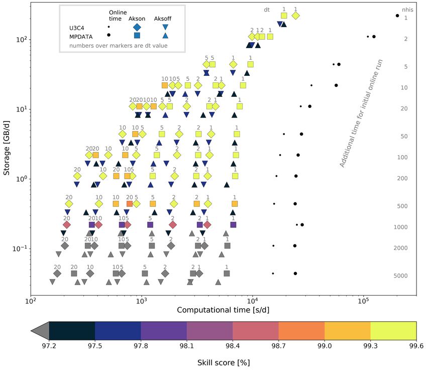
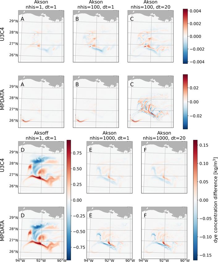
K. M. Thyng et al.: Performance of offline passive tracer advection in ROMS                                                               395

Figure 3. Instantaneous difference in dye concentration (online minus offline simulation) after about 13.2 d. Alternating rows show the results
from the two tracer advection schemes tested, and the columns show the different experiments. All pairs of experiments except D forced the
vertical salinity diffusion coefficient Aks. Experiment A vs. B shows the result of changing the forcing frequency of the online output into
the offline simulation, nhis, from 1 (every online time step) to every 100 online time steps for the online time step. Experiment C shows the
result of additionally changing the offline time step to be 20 times the online time step. Experiments E and F show offline experiments forced
with online output every 1000 online time steps with the offline time step of the online time step (dt = 1) or 20 times the online (dt = 20)
time step. Note that each color bar has a different range of values.

shown demonstrate the spread from the highest accuracy to                 decreases with increasing offline time step but in different
several levels down (nhis 200, 500, and 1000 times the on-                relative amounts that depend on the nhis value. For nhis
line time step, or about 1, 3, and 5.5 h, respectively). For each         of 200 and 500, there is more impact from the change in of-
nhis value, three different offline time steps, dt, are shown             fline time step dt than from the nhis value. However, for
(dt of 1, 10, and 20 times the online time step). Accuracy                nhis 1000, the dt values do not strongly impact the results.

https://doi.org/10.5194/gmd-14-391-2021                                                          Geosci. Model Dev., 14, 391–407, 2021
396                                             K. M. Thyng et al.: Performance of offline passive tracer advection in ROMS

Figure 4. Skill scores for several subsets of offline simulations. (a) Performance between the MPDATA and U3C4 tracer advection schemes
and whether the vertical salinity diffusion coefficient Aks is forced with the online simulation (“on”) or a constant background number
(“off”). These cases also have nhis=1 (the online output was saved each time step) and dt=1 (the offline time step matched the online time
step). (b) Performance between the MPDATA and U3C4 advection schemes with nhis values varying. These cases also have Aks forced
from the online case and dt=1. (c) Performance for varying nhis and dt parameters, where MPDATA is used and Aks is forced from the
online case. All offline simulations here are forced by his files.

Offline time step results for U3C4 simulations are not shown           ences in tracer advection. For comparison, the “skill score”
because the time step does not strongly impact results for any         comparing online U3C4 and online MPDATA output (gray
nhis values.                                                           dashed) is shown. The online–online comparison for the two
   Several issues are demonstrated in Fig. 5. First is an ex-          schemes has comparable performance, though lower; it is not
ample of model performance for a skill score based on per-             clear if there is a reason that the on- and offline combinations
sistence (Eq. 2). Model performance is similar, though a lit-          should be better or worse than this, but the issue was not fur-
tle lower, when assessed using the persistence skill score as          ther explored. The best fidelity to an online simulation will be
compared with the regular skill score, so it is only shown             found by forcing the offline simulation with the same tracer
here. This tells us that the offline model does indeed pro-            advection scheme as that used in the online simulation. Also,
vide more benefit than simply persisting the initial condition.        forcing the offline simulation with a different tracer advec-
Next is a demonstration of offline accuracy compared to on-            tion scheme from the online simulation will give results that
line output when different tracer advection schemes are used           are different from the online results on the order of the dif-
(Fig. 5b). For reference, simulations forced with the same             ference between the results of the different tracer advection
tracer advection schemes both on- and offline are shown as             schemes themselves. Finally, the significant impact of using
well (U3C4, black solid, and MPDATA, black dashed). We                 single-precision output is demonstrated (Fig. 5c); it is best to
find a significant decrease in offline model accuracy when the         save online model output for forcing offline simulations with
offline advection scheme does not match the online scheme,             double precision.
because different numerical schemes have different numer-                 Several other issues were investigated but not plotted (they
ical dispersion and diffusion properties leading to differ-            can be seen in the paper GitHub repository). Passive tracers

Geosci. Model Dev., 14, 391–407, 2021                                                     https://doi.org/10.5194/gmd-14-391-2021
K. M. Thyng et al.: Performance of offline passive tracer advection in ROMS                                                            397

Figure 5. (a) Skill score compared with persistence is shown for combinations of tracer advection schemes and whether online Aks is
forced. The simulations shown are the same as in Fig. 4a. (b) Comparison of skill score simulations forced by several combinations of tracer
advection schemes. The combinations are as follows: online simulation using U3C4 with offline simulation using U3C4 (black solid line),
online simulation using U3C4 with offline simulation using MPDATA (gray solid), online MPDATA with offline U3C4 (gray dashed) and with
offline MPDATA (black dashed), and a comparison between results from online U3C4 and online MPDATA (gray dotted). (c) Skill score for
double-precision compared with single-precision online output.

are conserved in online ROMS simulations (Shchepetkin and               quirements. For the present set of simulations, this occurs
McWilliams, 2005); offline simulations also conserve trac-              for U3C4 with realistic Aks for nhis of 200 (more conser-
ers. Only small differences were found between forcing of-              vative) or 500 and dt of 20, and for MPDATA with realistic
fline simulations with snapshots (his files) or averages be-            Aks for nhis 200 and dt of 5. Simulations in which Aks is
tween time steps (avg files) from online simulations. Finally,          not forced always have lower accuracy, and the small storage
for simulations in which a realistic Aks field was not forced,          saving is probably not worth the loss; however, there may be
the background value used for Aks was varied; we found that             circumstances in which online Aks is not available.
this did not impact results.
   An overview of results is shown in Fig. 6. The objective             3.2    At-depth realistic Gaussian
of this figure is to display the competing factors – com-
putation time (x axis) and storage required (y axis) – that             The biggest difference in the second set of simulations (ini-
will ultimately determine offline accuracy (colored mark-               tialization shown in Fig. 2) compared with the first is the
ers). Skill scores are shown for four subsets of simulations:           variation in the vertical direction: a dye blob was initial-
tracer advection scheme U3C4 with (diamonds) and with-                  ized at a particular depth instead of throughout the water col-
out (downward-pointing triangles) Aks realistically forced,             umn. A skill score comparison between 13 and 14 d indicates
and tracer advection scheme MPDATA with (squares) and                   that the good-resolution experiment (nhis = 100, or online
without (upward-pointing triangles) Aks realistically forced.           output forced in the offline simulation every ∼ 30 min) had
The best compromise between storage, computational time,                about the same skill score of 99.6 % as the comparable pre-
and skill score is where the skill score is still high – in one         vious numerical experiment skill score. However, the low-
of the top classes, but with the lowest storage and time re-            resolution test case (nhis = 1000, or online output forced

https://doi.org/10.5194/gmd-14-391-2021                                                        Geosci. Model Dev., 14, 391–407, 2021
398                                               K. M. Thyng et al.: Performance of offline passive tracer advection in ROMS

Figure 6. Summary of skill score results. Shown are the offline computational time per simulation day (x axis), the storage required for the
online simulation per simulation day (y axis), and the skill score after about 13.5 d of simulation when forcing with snapshots (his files) for
a range of nhis and dt values (colored markers, with one set for forcing Aks or not, and which tracer advection scheme is used). nhis
values for rows are indicated on the right-hand side of the plot, and dt values are shown above each pair of markers. Values below 97.2 %
are colored gray. The computational time required for the online simulation is shown separately with black markers.

every ∼ 5.5 h) had a much lower skill score of 70 % com-                  case percent error (Fig. 7g) with a swath of 1 %–10 % error
pared with the first test case of 98.5 %, possibly indicating a           across the full dye feature.
compensatory effect in the first set of experiments in the ver-              Results are similar for the vertical cross section (Fig. 8).
tical direction. That is, dye may have been transported verti-            The differences in the offline and online dye field are very
cally inaccurately in the first set of lower-resolution experi-           small in the good-resolution case – it has been multiplied by
ments, but as the whole water column had dye in it, it may                500 to appear on the same color bar as the low-resolution
have still given better skill scores than if the dye patch was            case. In the low-resolution case, the offline dye has been
instead discrete.                                                         transported both up and down more than in the online case.
   Spatial differences in the accuracy of the experiments are
shown for depth slices (Fig. 7) and cross sections (Fig. 8).
The dye in the good-resolution cases stays close to the online            4   Discussion
simulation, with small differences in the percent error near
where the dye encounters the bathymetry on the west end of                The context of the performance difference found as a func-
the blob (Fig. 7d and f, noting that the values in panel d have           tion of nhis values (Fig. 4b, c) can be considered as the
been multiplied by 100 to be visible). The low-resolution                 impact of loss of energy represented in the system (an ap-
case is qualitatively similar to the online case, but the dif-            proach also used by Qu and Hetland, 2019). For example,
ference (Fig. 7e) shows patches of large disagreement. The                Fig. 9 shows the power spectral density of the online simula-
disagreement is further demonstrated in the low-resolution                tion speed from near the middle of the dye patch. The output
                                                                          frequency, nhis, from the online simulation controls how

Geosci. Model Dev., 14, 391–407, 2021                                                        https://doi.org/10.5194/gmd-14-391-2021
K. M. Thyng et al.: Performance of offline passive tracer advection in ROMS 399
Figure 7. Snapshots of the dye at 13.75 d for the online (a), good-resolution offline (b), and low-resolution offline (c) simulations. The
difference in dye concentration for the online and offline cases at the same time for the good-resolution (d) and low-resolution (e) experiments.
The percent error for the good-resolution (f) and low-resolution (g) offline cases is also shown. Moreover, panel (a) indicates the slice location
shown in Fig. 8. Note that values in panel (d) have been multiplied by 100 to be visible on the same color bar as panel (e) as the differences
are so small.
much energy of this spectrum the offline simulations receive 1 % and 5 % of the total energy being lost to subsampling the
and, therefore, how much of the system’s energy is repre- output.
sented offline. The amount of energy missing can be seen Comparing a relevant dynamical timescale to nhis is an-
visually by the overlaid lines representing different output other way to provide context for its impact on offline accu-
frequencies, nhis. Skill score results (Fig. 4) show that ac- racy. A previous study evaluating an offline tracer from MIT-
curacy decreases as nhis values increase starting at nhis gcm model output found that for their global-scale model, the
of 200 or 500 (about 1 to 3 h), which correspond to between inertial period controlled the output rate necessary for robust
results (Hill et al., 2004). We find an analogous result here,
https://doi.org/10.5194/gmd-14-391-2021 Geosci. Model Dev., 14, 391–407, 2021400 K. M. Thyng et al.: Performance of offline passive tracer advection in ROMS Figure 8. Vertical cross section comparisons of the online and offline simulations; the cross section location is indicated in Fig. 7a. Snapshots at 13.75 d are shown for the online (a) and offline good-resolution (b) and low-resolution (c) cases. Differences at the same time are shown in panels (d) and (e). The percent error is shown in panels (f) and (g). Note that values in panel (d) have been multiplied by 500 to be visible on the same color bar as panel (e) as the differences are so small. though the relevant timescale is the advection timescale (see locity of 1 and the smallest horizontal cell width of about Sect. 2.1). The advection timescale for this regional model 3800 m, for the offline time steps gives a range from 0.005 is about 20 000 s, which corresponds to an output rate from for the offline time step matching the online time step up to the online model of nhis = 1000 times the online time step, about 0.1 and 0.25 for offline time step dt of 20 and 50, re- which is indeed the turning point for clear degradation in of- spectively. Simulations gave reasonable results for dt of 20 fline model accuracy we find (Fig. 6). but not for dt of 50. We should expect that the offline time step is controlled by the horizontal Courant number and that our results desta- bilize as the number increases toward 1. An estimate of the horizontal Courant number, with the largest horizontal ve- Geosci. Model Dev., 14, 391–407, 2021 https://doi.org/10.5194/gmd-14-391-2021
K. M. Thyng et al.: Performance of offline passive tracer advection in ROMS                                                          401

Figure 9. Power spectral density for speed at a single location near the center of the dye patch. Overlaid (gray dashed) are lines marking
frequencies at which online model output was saved for forcing offline simulations; these are marked with their corresponding nhis value.

5   Conclusions                                                        14 d). However, for MPDATA offline simulations were highly
                                                                       accurate with a time step 5 times the online time step up to
This paper presents a description and evaluation of an offline         nhis = 200, with some dependence on the offline time step.
tracer advection model developed within ROMS. The advan-                  A second set of simulations were run to demonstrate per-
tage of this is the ease and consistency with which ROMS               formance in a more realistic, application-driven experiment
users can employ existing model output to force offline tracer         – in this case, with a discrete blob of dye at depth. The
simulations at low computational cost. The main approach               good-resolution case with online forcing at a frequency of
of the offline model is to force variables zeta, u/v, and              nhis = 100 (about 30 min) was very accurate, with a sim-
ubar/vbar from an online simulation as climatology; nor-               ilar skill score to the original comparable offline U3C4 ex-
mally climatology would be used in a ROMS simulation to                periment run of 99.6 %. The low-resolution experiment of
nudge boundary conditions toward mean values, but in this              nhis = 1000 (about 5.5 h) gave worse results than the com-
case all grid cells are fully forced. Additionally forcing the         parable previous simulation, implying that the vertical di-
vertical salinity diffusivity, Aks, improves model accuracy.           rection is indeed important and can behave distinctly from
It is also important that the online simulation output used to         the horizontal. Overall, the results show that it is possible to
force the offline simulation has double precision.                     get high-fidelity results in offline tracer simulation with this
   We tested two tracer advection schemes, MPDATA and                  code.
TS_U3HADVECTION with TS_C4VADVECTION (third-
order upstream horizontal advection and fourth-order cen-
tered vertical advection, called U3C4 here), in a regional sim-
ulation of the northern Gulf of Mexico, and we found that the
offline simulations are able to reproduce online simulations
at a high accuracy. The most important control differentiat-
ing offline accuracy was the nhis parameter describing how
often online simulation output was saved, as a multiple of the
online time step, to be input into the offline simulation. For
both tracer advection schemes and with Aks forced, the of-
fline simulations showed high accuracy up to nhis = 200
or 500, about 1.1 and 2.8 h, respectively. This is consistent
with requiring temporal information at a rate higher than
the relevant dynamic timescale – in this case, an advection
timescale approximated as roughly equivalent to an nhis
value of 1000. The offline time step dt was not an impor-
tant choice for offline simulations run with U3C4, as long
as it was under about 50 (all had skill scores of 99.6 % after

https://doi.org/10.5194/gmd-14-391-2021                                                      Geosci. Model Dev., 14, 391–407, 2021
402 K. M. Thyng et al.: Performance of offline passive tracer advection in ROMS
Appendix A: Table of skill scores
Table A1. Final skill score (percent) of offline simulations after 14 d, sorted by nhis and dt values, tracer advection scheme, and if Aks is
forced.
Advect MPDATA U3C4
Aks Off On Off On
nhis dt
1 1 97.5 99.3 97.6 99.6
2 1 97.5 99.3 97.6 99.6
2 97.5 99.3 97.6 99.6
5 1 97.5 99.3 97.6 99.6
5 97.6 99.3 97.6 99.6
10 1 97.5 99.3 97.6 99.6
2 97.5 99.3 97.6 99.6
5 97.6 99.3 97.6 99.6
10 97.5 99.2 97.6 99.6
20 1 97.5 99.3 97.6 99.6
2 97.5 99.3 97.6 99.6
5 97.6 99.3 97.6 99.6
10 97.5 99.2 97.6 99.6
20 97.5 99.0 97.6 99.6
50 1 97.5 99.3 97.6 99.6
2 97.5 99.3 97.6 99.6
5 97.6 99.3 97.6 99.6
10 97.5 99.2 97.6 99.6
100 1 97.5 99.3 97.6 99.6
2 97.5 99.3 97.6 99.6
5 97.6 99.3 97.6 99.6
10 97.5 99.2 97.6 99.6
20 97.5 99.0 97.6 99.6
200 1 97.5 99.3 97.6 99.6
2 97.5 99.3 97.6 99.6
5 97.6 99.3 97.6 99.6
10 97.5 99.2 97.6 99.6
20 97.5 99.0 97.6 99.6
500 1 97.5 99.2 97.6 99.6
2 97.5 99.2 97.6 99.6
5 97.5 99.2 97.6 99.6
10 97.5 99.2 97.6 99.6
20 97.5 98.9 97.6 99.6
1000 1 96.9 98.0 97.2 98.5
2 96.9 98.0 97.2 98.5
5 96.9 98.0 97.2 98.5
10 96.9 98.0 97.2 98.5
20 96.9 97.9 97.2 98.5
2000 1 92.2 92.5 93.4 93.7
2 92.2 92.5 93.4 93.7
5 92.2 92.5 93.4 93.7
10 92.2 92.5 93.4 93.7
20 92.3 92.6 93.4 93.7
5000 1 78.2 78.3 79.4 79.6
2 78.2 78.3 79.4 79.6
5 78.2 78.4 79.4 79.6
10 78.2 78.4 79.4 79.6
20 78.3 78.4 79.4 79.6
Geosci. Model Dev., 14, 391–407, 2021 https://doi.org/10.5194/gmd-14-391-2021K. M. Thyng et al.: Performance of offline passive tracer advection in ROMS 403
Appendix B: Explanation of code changes – omega (OCLIMATOLOGY), which already existed and
does not impact offline tracer advection, reads in clima-
While preprocessor flags for offline simulations already ex- tology for the S coordinate vertical momentum compo-
isted in the ROMS and COAWST code base, we found that nent.
the offline simulations did not work as desired. In this sec-
– Aks (AKSCLIMATOLOGY), Akt
tion, we describe changes made to the code base so that of-
(AKTCLIMATOLOGY), and Akv
fline passive tracer advection works properly by receiving the
(AKVCLIMATOLOGY), or all three Aks, Akt, and Akv
necessary forced variables. Generally, the offline code works
(AKXCLIMATOLOGY) are new flags. Aks, the vertical
by forcing previously simulated online model output that is
salinity diffusion, impacts the accuracy of the offline
input as climatological forcing. Typically, climatology would
tracer (Sect. 3), whereas Akt, the vertical temperature
be used in a ROMS simulation to nudge boundary conditions
diffusion, does not impact offline tracer advection; the
toward mean values, but in this case all grid cells are fully
latter is used for offline floats (OFFLINE_FLOATS) if
forced.
vertical walk (FLOATS_VWALK) is activated. Akv, the
Code changes were made to avoid repeating processes
vertical viscosity, does not impact offline passive tracer
offline that were already included online. Initialization is
advection.
now minimal for offline simulations (ini_fields.F), and
initial values are replaced by the first time step read in – TKE (TKECLIMATOLOGY, turbulent kinetic energy),
from climatology. Updates to sea surface height zeta (calls GLS (GLSCLIMATOLOGY, generic length scale), or
to ini_zeta and set_zeta in main3d_offline.F) both
have been removed as the variable is directly forced in the (MIXCLIMATOLOGY) are new flags. These do not im-
offline simulation. Boundaries are not forced in the offline pact offline passive tracer advection.
case (except for the passive dye field): horizontal indices now
start one index earlier and end one index later in each tile so – salt and temp (ATCLIMATOLOGY) are new flags.
that climatology is read into ghost cells in place of bound- These flags are also impacted by LtracerCLM in the
ary conditions (set_data.F). The remaining processes are input file. While these do not impact offline tracer ad-
controlled through the user input file and preprocessor flags vection, they may be used for other modules such as oil
(Appendix C). modeling with offline floats.
The offline simulation is missing much of the com- To fix a problem with reading in the climatology at the cor-
plex time stepping in an online ROMS simulation due to rect time step, a condition was added (get_2dfld.F and
the missing numerics, leading to necessary code adjust- get_3dfld.F) that compares the differences in times to
ments (set_data.F). Climatology for 3D variables (u/v, being less than half a time step, avoiding any problems with
salt/temp, and tke/gls) are read into earlier time in- numerical precision.
dices (nrhs instead of nnew) to account for this, elim- omega, the mass flux perpendicular to the local S coor-
inating a time shift that otherwise occurs. Model out- dinate, was already set up to be read in through climatology
put for the subsequent time step are read in from cli- with the OCLIMATOLOGY flag, but results did not match on-
matology and saved in available time indices for sev- and offline. The lower vertical index in the call for omega
eral variables (zeta, Aks, and Akt) to be used later in get_data.F was one, which is used for rho grids in-
in the time loop. In the online simulation, zeta is nor- stead of the w-grid omega is actually on, which starts at in-
mally updated mid-time loop with the fast time-stepping dex zero.
value. To approximate this behavior, the two time steps of
zeta are averaged into variable Zt_avg1 (new function
set_avg_zeta). Calculations of vertical layer thickness Appendix C: How to set up simulations
Hz and mass fluxes Huon/Hvom for the subsequent time step
Requirements and considerations for setting up online and
are made mid-time loop in set_depth.F. New functions
offline simulations in ROMS or COAWST with the offline
set_massflux_avg and set_massflux_avg_tile
passive tracer advection code are provided below.
were added to set_massflux.F to average Huon/Hvom
values to be used subsequently in step3d_t.F where the C1 Online
tracer is advected. This change matches the online case to
floating-point round-off error. C1.1 Input file
The OFFLINE preprocessor flag with
OFFLINE_TPASSIVE compiles the necessary code to In the project input file (the *.in file, for exam-
run offline tracer advection (more details in Appendix C). ple, https://github.com/kthyng/oil_03/blob/master/External/
These flags already existed, but changes to the code for the ocean_oil_03.in, last access: 18 May 2020), the items below
present project were made under these flags. Other available should be considered in addition to the typical input parame-
offline preprocessor flags include ter selections:
https://doi.org/10.5194/gmd-14-391-2021 Geosci. Model Dev., 14, 391–407, 2021404 K. M. Thyng et al.: Performance of offline passive tracer advection in ROMS
– Choose whether to save output as snapshots at a sin- C2 Offline
gle time or averages across time intervals (ROMS his
vs. avg files). Your choice will be used to force the of- C2.1 Input file
fline simulation. Present results show that this choice
does not significantly change results. We recommend In the project input file (the *.in file, for exam-
using his files in the absence of any other preference ple, https://github.com/kthyng/oil_off/blob/master/External/
as if his files are not used, it is necessary to include the ocean_oil_offline.in, last access: 18 May 2020), the items
initial file prepended to the input avg file in CLMNAME. below should be considered in addition to the typical input
parameter selections:
– Output necessary variables for forcing the offline sim- – The output frequency (NHIS or NAVG) will not impact
ulation. Variables zeta, ubar, vbar, u, and v are your offline simulation performance, but it should be
required for forcing the offline simulation, and Aks is chosen to well represent the dynamics in your model.
optional for improved accuracy in the offline simulation
(though it increases amount of storage required). – A reasonable choice for the offline simulation time step
dt is a multiple of the online time step. Some testing
for your model setup is warranted. The present study
– Choose output frequency (parameter NHIS for his found that time step was not important for the U3C4
files or NAVG for avg files). This is how often ROMS tracer scheme combination – a dt of 20 times the online
will save output to a his or avg file, as a multiple time step gave accuracy which was as good as that for
of the time step, and in turn this is what will be used the online time step itself. However, for MPDATA, only
to force the offline simulation. Important considerations using the online time step gave the highest accuracy; for
for this selection include acceptable simulation runtime the next level down of accuracy, a time step of 10 times
and storage requirements. Figure 6 gives a paradigm the online time step was adequate (Fig. 6). Note also
from which to decide this for simulations in general. In that the offline time step needs to factor evenly into the
the present study, for U3C4 there was a drop in perfor- online output frequency, and the offline time step cannot
mance below an output frequency of 500 times the on- be larger than the online output frequency.
line time step, and below 200 or 500 times for MPDATA.
These choices will vary for a given model setup and ac- – All physics should be off in the offline case, except
curacy needs. for anything directly impacting the offline tracer field
(dye_01) itself, because it is included in the online out-
– For this online simulation, point to file put. This implies that
varinfo-online.dat for VARNAME, which – boundaries should all be closed except for offline
is a typical, unchanged file. This has been provided tracer fields, e.g., parameter LBC(isFsur);
in the code repository: https://github.com/kthyng/
COAWST-ROMS-OIL/blob/master/ROMS/External/ – river forcing and other sources or sinks that were
varinfo-online.dat (last access: 18 May 2020). forced in the online simulation should be turned off;
– winds, bulk fluxes, etc, should not be forced from
C1.2 Header file the online simulation;
– the model should not be nudged to climatology,
In the project header file (the *.h file, for example, https:// even if used in the online simulation (climatology,
github.com/kthyng/oil_03/blob/master/Include/oil_03.h, last the output from the online simulation, will be en-
access: 18 May 2020), the following additional flags should tirely enforced);
be considered:
– flags for climatology forcing for sea surface height
– Choose a tracer advection scheme. We tested two (LsshCLM) as well as 2D (Lm2CLM) and 3D mo-
schemes and found both accurately reproduced the on- mentum (Lm3CLM) should be turned on, and salt
line results offline, though U3C4 performed slightly bet- and temperature flags (LtracerCLM) should also
ter. Note, however, that online tracer advection perfor- be turned on if you want to read them in (see Ap-
mance itself depends on the dynamics involved; more pendix C2.2).
information is available in Kalra et al. (2019). Also note – Only the sea surface height (zeta) and the offline dye(s)
that MPDATA requires more runtime than U3C4 (Fig. 6). (dye_01) need to be output – other fields are best used
directly from the online simulation (the vertical velocity
– Use OUT_DOUBLE to output results with double preci- w, for example, is not calculated properly in the offline
sion to significantly improve your accuracy, though in- simulation). The sea surface height is necessary to prop-
crease storage is required (Fig. 5). erly calculate tracer advection fluxes.
Geosci. Model Dev., 14, 391–407, 2021 https://doi.org/10.5194/gmd-14-391-2021K. M. Thyng et al.: Performance of offline passive tracer advection in ROMS 405
– Input as the climatology forcing (CLMNAME) the online
model output. If forcing with an avg file from the on-
line simulation, it is necessary to place a file containing
the initial conditions first; this is possible by inputting a
list of file names.
– For this offline simulation, point to file
varinfo-offline.dat for VARNAME, which
has been edited to include the new variables that
can be input as climatology and so that all clima-
tology time variables are named ocean_time.
The latter change allows for the online output to
be input directly offline as climatology without
processing the file to rename variable attributes.
The file has been provided in the code repository:
https://github.com/kthyng/COAWST-ROMS-OIL/blob/
master/ROMS/External/varinfo-offline.dat (last access:
18 May 2020).
C2.2 Header file
In the project header file (the *.h file, for exam-
ple, https://github.com/kthyng/oil_off/blob/master/Include/
oil_offline.h, last access: 18 May 2020), the following ad-
ditional flags should be considered:
– Use the OFFLINE flag for any offline simulation and,
additionally, the OFFLINE_TPASSIVE flag for offline
tracer advection.
– For the best results, use the same tracer advection
scheme as the online run. The schemes do not have to
match, but the skill score between the simulations will
diminish substantially (Fig. 5) as they do not use the
same numerics. We did not test other tracer advection
schemes, but we have no reason to think they will not
work offline.
– Forcing the vertical salinity diffusivity Aks as predicted
by the online simulation gives better offline accuracy
than not forcing it, though it requires storing the infor-
mation from the online case. This can be forced with
the AKSCLIMATOLOGY flag. More information on the
offline flags is available in Appendix B.
https://doi.org/10.5194/gmd-14-391-2021 Geosci. Model Dev., 14, 391–407, 2021406 K. M. Thyng et al.: Performance of offline passive tracer advection in ROMS
Code and data availability. The current versions of the re- References
lated code and data are available online, all under the
MIT license. The offline tracer model is available from Azevedo Correia de Souza, J. M., Powell, B., Castillo-Trujillo,
https://github.com/kthyng/COAWST-ROMS-OIL (last access: A. C., and Flament, P.: The vorticity balance of the ocean sur-
3 November 2020); the analysis for this paper is avail- face in Hawaii from a regional reanalysis, J. Phys. Oceanogr.,
able from https://github.com/kthyng/offline_analysis (last 45, 424–440, 2015.
access: 17 November 2020); run files for online simula- Bogden, P. S., Malanotte-Rizzoli, P., and Signell, R.: Open-ocean
tions can be found at https://github.com/kthyng/oil_03 (last boundary conditions from interior data: Local and remote forc-
access: 19 August 2020); and run files for offline simula- ing of Massachusetts Bay, J. Geophys. Res.-Oceans, 101, 6487–
tions are available from https://github.com/kthyng/oil_off 6500, 1996.
(last access: 19 August 2020). The exact version of the Chassignet, E. P., Hurlburt, H. E., Smedstad, O. M., Halliwell,
model used to produce the results employed in this paper is G. R., Hogan, P. J., Wallcraft, A. J., Baraille, R., and Bleck, R.:
archived on Zenodo (https://doi.org/10.5281/zenodo.4455738, The HYCOM (hybrid coordinate ocean model) data assimilative
Thyng et al., 2021) as are the scripts to run the analy- system, J. Marine Syst., 65, 60–83, 2007.
ses and produce the plots for all of the simulations pre- Cummings, J. A.: Operational multivariate ocean data assimilation,
sented in this paper (https://doi.org/10.5281/zenodo.4278115, Q. J. Roy. Meteorol. Soc., 131, 3583–3604, 2005.
Thyng, 2020a), the run files for online simula- Cummings, J. A. and Smedstad, O. M.: Variational data assimila-
tions (https://doi.org/10.5281/zenodo.4455715, Thyng, tion for the global ocean, in: Data Assimilation for Atmospheric,
2020b), and the run files for offline simulations Oceanic and Hydrologic Applications (Vol. II), pp. 303–343,
(https://doi.org/10.5281/zenodo.4455760, Thyng and Ruiz Springer, Berlin, Heidelberg, 303–343, 2013.
Xomchuk, 2021). Input data to run the model are available both Dutkiewicz, S., Follows, M., Marshall, J., and Gregg, W. W.: In-
on figshare (https://doi.org/10.6084/m9.figshare.c.5097350.v1, terannual variability of phytoplankton abundances in the North
Thyng et al., 2020a) and through the Gulf of Mexico Re- Atlantic, Deep-Sea Res. Pt. II, 48, 2323–2344, 2001.
search Initiative Information and Data Cooperative (GRIIDC; Fairall, C. W., Bradley, E. F., Hare, J., Grachev, A. A., and Edson,
https://doi.org/10.7266/YF0QPBFC, Thyng et al., 2020b). Simu- J. B.: Bulk parameterization of air–sea fluxes: Updates and verifi-
lation output from the online and offline simulations is available cation for the COARE algorithm, J. Climate, 16, 571–591, 2003.
through GRIIDC (https://doi.org/10.7266/7R0N3FX4, Thyng, Fox, D., Teague, W., Barron, C., Carnes, M., and Lee, C.: The mod-
2020c). ular ocean data assimilation system (MODAS), J. Atmos. Ocean.
Tech., 19, 240–252, 2002.
Gillibrand, P. A. and Herzfeld, M.: A mass-conserving advection
Author contributions. KMT edited the code, performed the final scheme for offline simulation of scalar transport in coastal ocean
simulations and analysis, and wrote the text. DK, VRX, and LQ models, Ocean Model., 101, 1–16, 2016.
edited the ROMS code and ran simulations. XC created the regional Hetland, R. D.: Event-driven model skill assessment, Ocean Model.,
model setup in ROMS. RDH participated in discussions and pro- 11, 214–223, 2006.
vided ideas. Hill, H., Hill, C., Follows, M., and Dutkiewicz, S.: Is there a com-
putational advantage to offline tracer modeling at very high res-
olution, Researchgate, Geophys. Res. Abstr., 6, 2004.
Hoyer, S. and Hamman, J.: xarray: N-D labeled Arrays
Competing interests. The authors declare that they have no conflict
and Datasets in Python, J. Open Rese. Softw., 5, 10,
of interest.
https://doi.org/10.5334/jors.148, 2017.
Hunter, J. D.: Matplotlib: A 2D graphics environment, Comput. Sci.
Eng., 9, 90–95, 2007.
Acknowledgements. This research was made possible by a Kalra, T. S., Li, X., Warner, J. C., Geyer, W. R., and Wu, H.: Com-
grant from the Gulf of Mexico Research Initiative. In ad- parison of Physical to Numerical Mixing with Different Tracer
dition to the locations noted in the “Code and data avail- Advection Schemes in Estuarine Environments, J. Marine Sci.
ability” section, data are publicly available through the Gulf Eng., 7, 338, https://doi.org/10.3390/jmse7100338, 2019.
of Mexico Research Initiative Information and Data Coop- Khatiwala, S., Visbeck, M., and Cane, M. A.: Accelerated sim-
erative (GRIIDC) at https://data.gulfresearchinitiative.org (last ulation of passive tracers in ocean circulation models, Ocean
access: 21 January 2021) (https://doi.org/10.7266/YF0QPBFC, Model., 9, 51–69, 2005.
https://doi.org/10.7266/7R0N3FX4). Kluyver, T., Ragan-Kelley, B., Pérez, F., Granger, B. E., Bussonnier,
The authors are grateful to the Texas A&M High Performance M., Frederic, J., Kelley, K., Hamrick, J. B., Grout, J., Corlay, S.,
Research Computing center for hosting simulations. and Ivanov, P.: Jupyter Notebooks-a publishing format for repro-
ducible computational workflows, ELPUB, 87–90, 2016.
Lévy, M., Resplandy, L., Klein, P., Capet, X., Iovino, D., and Éthé,
Financial support. This research has been supported by the Gulf of C.: Grid degradation of submesoscale resolving ocean models:
Mexico Research Initiative (grant no. SA 18-10). Benefits for offline passive tracer transport, Ocean Model., 48,
1–9, 2012.
McKinley, G. A., Follows, M. J., and Marshall, J.: Mechanisms
Review statement. This paper was edited by Qiang Wang and re- of air-sea CO 2flux variability in the equatorial Pacific and the
viewed by two anonymous referees. North Atlantic, Global Biogeochem. Cycles, 18, 2004.
Geosci. Model Dev., 14, 391–407, 2021 https://doi.org/10.5194/gmd-14-391-2021K. M. Thyng et al.: Performance of offline passive tracer advection in ROMS 407 McKinney, W.: Data Structures for Statistical Computing in Thyng, K., Chen, X., and Morey, S.: ROMS Input Files Python, in: Proceedings of the 9th Python in Science Confer- (second source), Gulf of Mexico Research Initiative In- ence, edited by: van der Walt, S. and Millman, J., pp. 56–61, formation and Data Cooperative (GRIIDC), Harte Re- https://doi.org/10.25080/Majora-92bf1922-00a, 2010. search Institute, Texas A&M University – Corpus Christi, Qu, L. and Hetland, R. D.: Temporal resolution of wind forcing https://doi.org/10.7266/YF0QPBFC, 2020b. required for river plume simulations, J. Geophys. Res.-Oceans, Thyng, K., Kobashi, D., Ruiz Xomchuk, V., Qu, L., Chen, X., and 124, 1459–1473, 2019. Hetland, R. D.: Offline passive tracer in ROMS (Version v1.1), Saha, S., Moorthi, S., Pan, H. L., Wu, X., Wang, J., Nadiga, S., Zenodo, https://doi.org/10.5281/zenodo.4455738, 2021. Tripp, P., Kistler, R., Woollen, J., Behringer, D., and Liu, H.: Thyng, K. M., Greene, C. A., Hetland, R. D., Zimmerle, H. M., and The NCEP climate forecast system reanalysis, B. Am. Meteorol. DiMarco, S. F.: True Colors of Oceanography: Guidelines for Soc., 91, 1015–1058, 2010. Effective and Accurate Colormap Selection, Oceanography, 29, Shchepetkin, A. F. and McWilliams, J. C.: The regional 9–13, 2016. oceanic modeling system (ROMS): a split-explicit, free-surface, Virtanen, P., Gommers, R., Oliphant, T. E., Haberland, M., Reddy, topography-following-coordinate oceanic model, Ocean Model., T., Cournapeau, D., Burovski, E., Peterson, P., Weckesser, W., 9, 347–404, 2005. Bright, J., van der Walt, S. J., Brett, M., Wilson, J., Jarrod Mill- Thyng, K.: kthyng/offline_analysis: Revised run files for offline man, K., Mayorov, N., Nelson, A. R. J., Jones, E., Kern, R., Lar- passive tracer simulation in ROMS (Version v1.1), Zenodo, son, E., Carey, C., Polat, İ., Feng, Y., Moore, E. W., Vand erPlas, https://doi.org/10.5281/zenodo.4278115, 2020a. J., Laxalde, D., Perktold, J., Cimrman, R., Henriksen, I., Quin- Thyng, K.: Run files for online simulation (Version v1.1), Zenodo, tero, E. A., Harris, C. R., Archibald, A. M., Ribeiro, A. H., Pe- https://doi.org/10.5281/zenodo.4455715, 2020b. dregosa, F., van Mulbregt, P., and Contributors: SciPy 1.0: Fun- Thyng, K.: Output from running offline passive tracer in damental Algorithms for Scientific Computing in Python, Na- ROMS ocean model, Gulf of Mexico Research Initiative ture Methods, 17, 261–272, https://doi.org/10.1038/s41592-019- Information and Data Cooperative (GRIIDC), Harte Re- 0686-2, 2020. search Institute, Texas A&M University – Corpus Christi, Warner, J. C., Armstrong, B., He, R., and Zambon, J. B.: Devel- https://doi.org/10.7266/7R0N3FX4, 2020c. opment of a coupled ocean–atmosphere–wave–sediment trans- Thyng, K. and Ruiz Xomchuk, V.: Run files for offline pas- port (COAWST) modeling system, Ocean Model., 35, 230–244, sive tracer simulation in ROMS (Version v1.1), Zenodo, 2010. https://doi.org/10.5281/zenodo.4455760, 2021. Zhang, Y., Jaeglé, L., and Thompson, L.: Natural biogeochemi- Thyng, K., Chen, X., and Morey, S.: ROMS input files, figshare, cal cycle of mercury in a global three-dimensional ocean tracer Collection, https://doi.org/10.6084/m9.figshare.c.5097350.v1, model, Global Biogeochem. Cycles, 28, 553–570, 2014. 2020a. https://doi.org/10.5194/gmd-14-391-2021 Geosci. Model Dev., 14, 391–407, 2021
You can also read