Soft Real-Time Scheduling in Google Earth
←
→
Page content transcription
If your browser does not render page correctly, please read the page content below
Soft Real-Time Scheduling in Google Earth
Jeremy P. Erickson University of North Carolina at Chapel Hill
Greg Coombe Google, Inc.
James H. Anderson University of North Carolina at Chapel Hill
Abstract
Google Earth is a virtual globe that allows users
to explore satellite imagery, terrain, 3D buildings, and
geo-spatial content. It is available on a wide variety
of desktop and mobile platforms, including Windows,
Mac OS X, Linux, iOS, and Android. To preserve the
sense of fluid motion through a 3D environment, the ap-
plication must render at 60Hz. In this paper, we dis-
cuss the scheduling constraints of this application as a
soft real-time scheduling problem where missed dead-
lines disrupt this motion. We describe a new scheduling
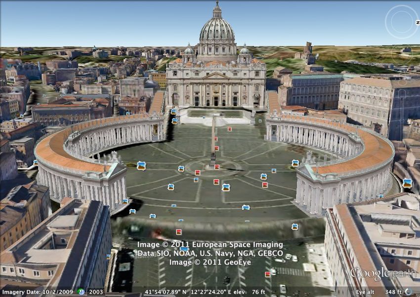
implementation that addresses these problems. The di- Figure 1: Google Earth screenshot of St. Peter’s Basil-
versity of hardware and software platforms on which ica from Sightseeing Tour.
Google Earth runs makes offline execution time analy-
sis infeasible, so we discuss ways to predict execution
time using online measurement. We provide experimen- the technique of altering level-of-detail (LOD) is pro-
tal results comparing different methods for predicting posed to ensure consistent frame rates. The authors
execution time. This new implementation is slated for propose certain heuristics in order to estimate rendering
inclusion in a future release of Google Earth. time, the time required to render a single frame. In [12]
these heuristics are explored in more detail and hard-
ware extensions are proposed that can be used to enable
1. Introduction soft real-time scheduling. Due to the hardware require-
ments, these techniques cannot be used for an applica-
Google Earth is a 3D graphics application used by tion such as Google Earth that needs to run on a wide
millions of consumers daily. Users navigate around range of existing consumer devices. For the specific
a virtual globe and can zoom in to see satellite im- case of mobile devices, rendering time analysis meth-
agery, 3D buildings, and data such as photos and links to ods are presented in [7, 10]. Although Google Earth
Wikipedia. An example screenshot is shown in Fig. 1. does currently alter LOD, for this paper we focus on the
In addition to a free edition, professional editions exist complementary approach of delaying problematic jobs
for use by corporations and governments. Such editions to future frames. Therefore, rather than predicting how
are used in broadcasting, architecture, environmental the workload will be reduced when the LOD is reduced,
monitoring, defense, and real estate for visualization we need accurate predictions for how long jobs will take
and presentation of geo-spatial content. When navigat- to run. Furthermore, existing work applies detailed pre-
ing the globe, an illusion of smooth motion should be diction mechanisms only to rendering jobs that execute
created. However, the application currently has a signif- primarily on the GPU, whereas we are also interested in
icant amount of visible stutter, a phenomenon in which CPU-bound and network-bound jobs.
the display fails to update as frequently as it should. In this paper, we provide methods to predict the
Several techniques have been proposed to address execution time of these jobs. The wide variety of tar-
the problem of stutter in graphics applications. In [1] get platforms make offline analysis of execution timeimpractical, so the execution time of jobs must be pre- vsync event, but missing it introduces artifacts by re-
dicted based on online statistical collection. Further- drawing the previous frame. This causes a noticeable
more, Google Earth has a limited preemption model discontinuity in the motion, known as stutter. See [8]
(described in Sec. 2.1). These issues make reducing for a discussion of the perceptual impact of stutter.
stutter difficult, particularly without negatively affect- The Google Earth process consists of multiple
ing the response time of jobs (see Sec. 2). The primary threads, each with its own context and execution path,
contribution of this paper is an implementation study of but all of which are part of the same process and share
different methods to predict execution times for hetero- common memory. The first thread started by the operat-
geneous sets of jobs, with the goal of reducing stutter ing system, and running the main function, is called the
with minimum effect on response times. We propose a main thread. Due to the requirements of the graphics
simple prediction mechanism that can significantly re- drivers on some systems that Google Earth supports, all
duce stutter. direct access to the graphics hardware must take place
Our new scheduler implementation is planned for within the main thread. For the purposes of this paper,
inclusion in a future release of Google Earth. Thus, we only consider the work executed on the main thread.
it requires careful planning and testing to ensure that A scheduler is a unit of code that repeatedly calls
users, particularly paying customers, do not experience certain functions based on scheduling constraints. Each
any loss of functionality. One difficulty in this regard function that is called constitutes a task, and each call to
is the requirement that the implementation be done “in- the function is a job. (A job can make its own function
place” without disrupting the existing behavior (due to a calls, which are considered part of the job.) A job is
planned production release halfway through this work). released when it is added to the scheduler for execution.
As changing the scheduling logic could have complex Each frame requires three stages of execution
unforeseen consequences, the new scheduler must be within the main thread, as depicted in Fig. 2. Ini-
capable of mimicking the existing behavior. This was tially, static jobs are run in a specific order dictated by
complicated by the fact that the existing code was not data dependencies. These include traversing data struc-
designed with a clear notion of scheduling, resulting in tures to perform updates and culling, uploading data to
several different ad-hoc methods. the graphics card, handling input events, etc. An ex-
In Sec. 2, we describe the terminology and task ample of a typical frame is given in Sec. 2.2. Then,
model used in this paper. Our description of the new the dynamic scheduler considered here is invoked and
scheduling implementation is given in Sec. 3, followed runs dynamic jobs, described in more detail in Sec. 2.3.
by descriptions of specific time-prediction algorithms in (Note: This work focuses on the dynamic scheduler.
Sec. 4, and experimental results in Sec. 5. Therefore, when “scheduler” is used without qualifica-
tion, it refers to the dynamic scheduler, and when “job”
2. Background is used without qualification, it refers to a dynamic job.)
Finally, the vsync function is called. The purpose of
In Sec. 2.1, we describe the constraints that the ap- the vsync function is to let the graphics hardware know
plication runs under and define relevant terms used in that there is a new image ready for the vsync event, and
this paper. In Sec. 2.2 we provide an example schedule it works by blocking until the next vsync event has com-
to motivate the task model, and in Sec. 2.3, we describe pleted and then returning. Observe that whenever the
the task model. vsync function is started, it completes at the next vsync
event, and starting the vsync function at the wrong time
2.1. Definitions results in blocking the main thread for a large amount
of time, as occurs in Frame 3 in Fig. 2. We say that a
Each image rendered on the screen is called a vsync event is successful if the main thread is running
frame. The illusion of smooth motion is created by ren- the vsync function when it occurs, and unsuccessful oth-
dering these frames at a sufficiently high rate. Due to erwise. To attempt to ensure that the next vsync event
the synchronization of commodity graphics hardware is successful, when the dynamic scheduler is run, it is
and the display device, the frame rate is a fixed amount given a scheduler deadline to complete by. The sched-
(usually 60 Hz. for desktop machines). This means that uler deadline is before the vsync event so that there is
all of the work to process and render a single frame enough time for the overhead of returning from the dy-
must be completed in 1/60th of a second, which gives namic scheduler and calling the vsync function. In the
a frame period of 16.67ms. A frame period boundary is absence of overheads, the scheduler deadline would be
known as a vsync event (from vertical synchronization). at the vsync event.
There is no benefit to completing rendering before the From the user’s perspective, a job’s completion isMain Event Loop
Static Jobs
Dynamic Scheduler ...
Dynamic Jobs
Vsync
Frame 1 Frame 2 Frame 3
Execution (different vertical positions
Vsync event Function Call Return From Function Scheduler Deadline
or fill colors means different functions)
Figure 2: Execution path within the main thread. Sizes and numbers of jobs are simplified for illustration.
Job 1
(from the start of the job until its first PP) is the ini-
Unsuccessful
Vsync! tial NP section, and each NP section thereafter (between
Job 2
two PPs or between a PP and the job completion) is a
post-PP NP section. Within the set of post-PP NP sec-
Execution Release
Vsync Event tions within a job, the longest (or an arbitrary longest
(Frame Boundary)
in case of a tie) is referred to as the longest post-PP NP
section. Each job contains exactly one initial NP sec-
Figure 3: Both Job 1 and Job 2 have perceived response tion, zero or more post-PP NP sections, and at most one
times of 2 frames, due to the unsuccessful vsync event longest post-PP NP section.
caused by Job 2.
A predictor is an object that has two functions: one
that inputs task ID, NP section type, and NP section
length for each initial or longest post-PP NP section and
not visible until the next successful vsync event. There-
updates internal state, and one that outputs a prediction
fore, we define a job’s perceived response time as the
for the next NP runtime given task ID and NP section
number of (complete or partial) frame periods between
type. (The longest post-PP NP section is used to pre-
its release and the next successful vsync event after its
dict all post-PP NP sections. This decision is explained
completion, as shown in Fig 3. For example, if a job
in Sec. 4.) A predictor type describes the particular
is released and completes between two vsync events,
method used to produce predictions given the inputs.
and the second vsync event is successful, its perceived
Particular predictor types are described in Sec. 4.
response time is one frame period. The perceived re-
sponse time of each job should be as short as possible. A soft deadline is a deadline that can be missed,
However, because stutter is more noticeable to the user but should be missed by a reasonably small amount.
than a delay of even a few seconds, avoiding an unsuc- There is still value in completing a job after its dead-
cessful vsync event is generally a higher priority than line has passed. Similar constraints have been discussed
achieving a small perceived response time. We discuss in [9]. A firm deadline is a deadline after which a job
this tradeoff in more detail in Secs. 4 and 5. should not be completed, but should instead be dis-
carded. Missing a firm deadline is costly, but not catas-
trophic.
* *(Preempted) * *
Initial NP Longest Post-PP NP Section
Section 2.2. Example Schedule
* Preemption Point (PP)
Post-PP NP Sections To understand the workload of Google Earth, it is
helpful to understand some of the work needed to cre-
Figure 4: NP section types. ate a single frame for rendering. An example schedule
(with parameters chosen for illustration rather than re-
A point where a job can be preempted is called a alism) is depicted in Fig. 5. Based on the camera po-
preemption point (PP), first described in [11]. (Our spe- sition, the Visibility Computation creates a list of visi-
cific implementation of preemption points is discussed ble regions and compares it to the existing regions. If
in Sec. 3.) We divide each job into non-preemptive (NP) regions are not currently loaded or are at a different
sections based on its PPs. There are two NP-section resolution, the same job queues up a fetch to request
types, depicted in Fig. 4. The first NP section of a job each needed region. In our example, there are two suchFrame 1 Frame 25 Frame 26
Static Jobs
(Outside scheduler)
Deadline
Visibility Computation
* *
**
...
Miss
(Sporadic)
Fetch 1
(Aperiodic) *
Fetch 2
(Aperiodic)
Road Drawing
(Sporadic)
time
Preemption Unavailable Vsync Event Scheduler
* point time
Execution Release Deadline (Frame Boundary) Deadline
Figure 5: Example task system with simplified parameters chosen for illustration.
regions. When the server responds, each of these re- quently as possible while having at most one job exe-
gions is processed (decoded, loaded into texture mem- cuting during each frame.) The soft deadline of each
ory, inserted into the data structures, stored in a cache, job is defined to be the next vsync event, so that in the
etc.); in Fig. 5 this per-region processing is denoted as ideal case each job has a perceived response time of one
Fetch 1 and Fetch 2. This new data can cause a num- frame and a job is released at each vsync event. A soft
ber of other data structures to be updated. For example, real-time (SRT) aperiodic task, on the other hand, has
higher resolution terrain data requires updating the alti- jobs released in response to I/O events, such as receiv-
tudes of the road segments — Road Drawing. Observe ing new imagery over the network. In the example dis-
that, due to the preemption model, idleness is present cussed in Sec. 2.2, Fetch 1 and Fetch 2 are SRT aperi-
at the end of each frame period to avoid missing the odic tasks. Because large amounts of data may be re-
scheduler deadline (and, in turn, risking an unsuccess- quested at the same time and network behavior is some-
ful vsync event). Also observe the large variance in ex- what unpredictable, no constraints exist on the release
ecution times. For example, the Road Drawing task re- times of such tasks. However, because new data usually
quires more work when new data has been processed. indicates that the view on the screen needs updating, the
The amount of time left after the static jobs varies dra- timing of their jobs is also important. Therefore each
matically between frame periods. The dynamic sched- job of an SRT aperiodic task also has a soft deadline
uler must account for this variation. at the next vsync event after it is released. A job of an
SRT aperiodic task can be canceled if the application
determines that it is no longer relevant. (For example, a
2.3. Task Model
network response with details about a 3D building that
is no longer in view does not need to be processed.)
There are two types of tasks with dynamic jobs in
Google Earth. A single-active sporadic (SAS) task has Furthermore, for analysis purposes, we can model
one job released at each vsync event, unless another job the vsync event as a periodic task with an execution time
of the task has been released (at a previous vsync event) of ε (for an arbitrarily small ε) and a period of 16.67 ms
but has not yet completed. In our example discussed in (assuming a 60 Hz refresh rate), with a firm deadline at
Sec. 2.2 the Visibility Computation is an SAS task that the vsync event and released ε units before. This peri-
misses its deadline at the end of frame 25, and so does odic task represents the time when the vsync function
not release a new job for frame 26. The Road Drawing needs to be called. Any time that the vsync function
task is also an SAS task, but meets all of its deadlines runs past the vsync deadline is modeled as unavailable
and therefore releases a job at every vsync event. The time like the static jobs that follow it. Meeting the dead-
requirement that there be only one job that has been re- line of the periodic vsync task corresponds to a success-
leased but not completed is a simple form of adaptivity ful vsync event, while missing it corresponds to an un-
that limits the load of the system. (More complex adap- successful vsync event. If tasks were fully preemptible,
tivity schemes exist, e.g. [4], but this simple scheme is meeting this task’s firm deadline would be trivial, but
used to ensure that each SAS task releases jobs as fre- due to the limited preemption model we must ensurethat no other job is running when the deadline occurs. ends the scheduler’s execution as well, and no further
jobs are scheduled before the vsync event.
3. Implementation
In this section, we describe the implementation of a 3.2. New Implementation
soft real-time scheduler within the legacy Google Earth
codebase. First we describe, in Sec. 3.1, the existing im-
plementation of task scheduling in Google Earth. Then, For this work, we have implemented a new
in Sec. 3.2, we discuss the new implementation. scheduling interface for Google Earth, which is in-
cluded in a preliminary form in Google Earth 6.1 and
Scheduler:: will be included in a more complete form in a future
Run
release of Google Earth. We have a new interface
IJobScheduler, as shown in Fig. 7. As with the old
Job: * * * scheduler implementation, we continue to use FIFO to
prioritize jobs. (Observe that, by our task model, FIFO
Preemption Scheduler Vsync Function Function
is equivalent to EDF with appropriate tie-breaking.) Al-
* Point Deadline Event Call Return
though the prioritization of jobs is identical in our new
(a) Existing scheduler relies upon jobs to do their own time scheduler, the behavior has significant differences. For
accounting at their preemption points. This often causes un-
successful vsync events. one, instead of relying on jobs to avoid scheduler dead-
line misses, the scheduler does not execute a job if it
Scheduler:: predicts it will cause a scheduler deadline miss, and
Run stops executing jobs if the scheduler deadline is actu-
Job * * ally missed, as shown in Fig. 6(b). The new scheduler
T F
uses a predictor (predictors are defined in Sec. 2.1) to
Scheduler:: T = True
ShouldContinue F = False
determine whether each NP interval is likely to cause a
scheduler deadline miss. (If the current time plus the
Preemption Scheduler Vsync Function Function
* Point Deadline Event Call V Returns V NP section prediction exceeds the scheduler deadline,
(b) Jobs now contain explicit preemption points that call back
then the job is predicted to cause a scheduler deadline
to the scheduler through a function ShouldContinue. The miss.) Specific predictor types are discussed in Sec. 4.
scheduler then uses online prediction to determine whether to Unlike the previous scheduler, the new scheduler does
execute jobs, and if it returns “false,” the job returns. If the not stop executing when the predictor indicates a sched-
job is unlikely to finish before the scheduler deadline, then it is
postponed until the next frame period. uler deadline miss, but instead executes remaining jobs
(with shorter predicted NP sections) that are not ex-
Figure 6: A similar job under the (a) old and (b) pected to cause scheduler deadline misses. In order to
new schedulers. Moving the preemption control to the prevent starvation of jobs that have very long predicted
scheduler enables advanced prediction models. NP section times, a non-starvation rule is applied: when
the scheduler begins its execution for a particular frame,
it always executes the highest-priority job (by FIFO),
3.1. Existing Implementation regardless of whether that job is predicted to cause a
scheduler deadline miss.
In Google Earth version 6.0 and prior, the scheduler
is passed the scheduler deadline, which is then passed to A more direct preemption mechanism is also in-
the jobs. Jobs are scheduled in simple FIFO order. The cluded in the IJobScheduler interface. When a
scheduler ceases executing when a job detects that it is job can safely be preempted, it can call a function
past the deadline, as shown in Fig. 6(a). Jobs check for ShouldContinue on the scheduler, optionally in-
actual or expected deadline misses only at points where cluding a prediction for how much time it expects to
they can safely be preempted. run before it next calls ShouldContinue or com-
A small number of jobs use time prediction to avoid pletes. The scheduler will determine whether the job
scheduler deadline misses. As these jobs process el- needs to be preempted and returns its decision to the
ements from a work queue, they maintain a running job. This approach allows us to use existing PPs and/or
average of per-element execution times. If the aver- time predictions where present, but we must modify all
age exceeds the available time before the deadline, they existing jobs by replacing deadline checks with calls to
will voluntarily give up execution. This self-preemption ShouldContinue.class IJobScheduler { 800
void AddJob(job);
700
void RunJobs();
bool ShouldContinue(job); 600
Occurrences
500
class Job {
400
bool Run();
TaskID GetTaskID(); 300
}; 200
100
class TimePredictor {
0
double Predict( 0 0.02 0.04 0.06 0.08 0.1
task_id, np_section_type); Milliseconds
void RecordExecutionTime(
task_id, np_section_type, time); Figure 8: Histogram of initial NP section length for one
}; task with the tail of the histogram truncated at 0.1 ms.
}; The worst case for this task is 15 ms. Many of the tasks
in Google Earth exhibit this long-tail behavior.
Figure 7: Interface for the implementation of new
scheduler. such a time prediction (which is the case precisely for
jobs that implemented time prediction in version 6.0),
the scheduler will also call its associated predictor, and
4. Time Predicton will operate based on the more pessimistic (i.e., larger)
result. Pessimism can therefore only increase. We study
As discussed in Sec. 3, the new Google Earth the improvement available by adding predictions that
scheduler uses predictors to estimate NP section length. did not previously exist, and are not concerned with the
Choosing an appropriate predictor type is essential for accuracy of predictions already present.
performance. Here we see the competition between Because initial NP sections and post-PP NP sec-
scheduler deadline misses and perceived response time: tions are likely to involve different code paths, their tim-
if the predictor is too optimistic, it can result in large ing statistics are handled separately. Code paths for dif-
numbers of scheduler deadline misses, but if it is too ferent post-PP NP sections may or may not differ within
pessimistic, it can result in large perceived response a job, so we use the longest post-PP NP section when
times (because jobs are deferred to later frame periods). predicting any post-PP NP section time.
Scheduler deadline misses can also increase perceived We now describe the predictor types tested in this
response time by causing an unsuccessful vsync event, work. Experimental results are given in Sec. 5.
as jobs that completed before the unsuccessful vsync
event will not have their effects observed until the next No Scheduler Prediction. In order to mimic the be-
successful vsync event. havior of the Google Earth 6.0 scheduler as closely as
Accurate time prediction is complicated by the ir- possible, one implementation of time prediction is sim-
regular distributions of NP section lengths for each par- ply to predict a time of 0 for each NP section of any
ticular task. A histogram of the initial NP section length type. If a job does not provide its own time prediction,
for one particular task, measured from actual execution, then it will be scheduled unless the scheduler deadline
is depicted in Fig. 8. The largest observed execution has already been missed.
for this task is 15 ms, but its average execution is far When using this predictor type, we sometimes
smaller. If the predictor predicts shorter than 15 ms for modify the scheduler to return to the top level as soon
initial NP sections of this job, then a scheduler dead- as it decides not to schedule a particular job, to emu-
line miss is possible. However, if the predictor predicts late the behavior of Google Earth 6.0 more precisely.
15 ms or larger, then jobs of this task are likely to be (Recall, as discussed in Sec. 3, that the new scheduler
delayed more frequently than necessary. will normally attempt to schedule a job with a shorter
NP section prediction in this case.) This technique is
In this section we discuss several predictor types,
referred to as 6.0 emulation.
with a brief description of the rationale for each. In
each case, the scheduler also supports receiving time Maximum Observed Execution. For a worst-case
predictions from the job itself. If a job does provide execution time estimate, one metric is to use the maxi-mum observed execution time for each type of NP sec- 80000
tion. While this method provides an obvious metric for 70000
“worst-case execution time,” it has the problem that it is
60000
highly sensitive to outliers. For example, if the operat-
ing system decides to preempt Google Earth during the 50000
Jobs
execution of a job, then the measured NP section length 40000
could be very large. Pessimistically assuming that all
30000
jobs of the same task can require such a large amount of
execution time could result in large delays, and a large 20000
perceived response time for such jobs. Simple outlier 10000
detection methods are difficult to apply due to the ir- 0
regular long-tailed distributions (as in Fig. 8) that these 0 10 20 30 40 50
jobs exhibit even when functioning normally. There- Frames
fore, we instead allow values to expire, so as to limit
the amount of time when a true outlier will have no- Figure 9: Typical perceived response histogram.
ticeable effects. For example, we can use the worst ob-
served response time over the past six seconds instead
5. Experiments
of since the start of the application. If Google Earth is
preempted while executing some job, then the relevant
In order to evaluate the tradeoffs between differ-
task will be penalized for only the next six seconds.
ent predictor types, we performed experiments using
NP Section Time Histogram. If we minimize the a modified version of the “Sightseeing Tour” shipped
probability of predicting too small an NP section time, with Google Earth. The Sightseeing Tour shows a vari-
then we risk creating large perceived response times. ety of scenes across the planet such as the Eiffel Tower,
Instead, we consider the approach of targeting a specific St. Peter’s Basilica (shown in Fig 1), downtown Sydney,
small probability of such mispredictions. In order to do and the Google campus in Mountain View, California.
so, we can store a histogram of past NP section times. This particular tour makes heavy use of demanding fea-
We use a bin size of 10−3 milliseconds, and allow a con- tures such as 3D buildings, so it exposes behavior that
figurable percentile of the histogram to be selected. For is likely to be worse than will be observed during typ-
example, if using a 95% histogram, the leftmost 95% ical interactive use. In the tour provided with Google
of values will be selected, and the maximum value in Earth, there are pauses built into the tour at each major
the appropriate bin range used as an execution time es- landmark, allowing the user to see the scene until they
timator. The target in this case is a 5% probability of manually restart the tour. To facilitate testing, we re-
misprediction. Maintaining the histogram does require moved these pauses from the tour, so that all landmarks
substantially more overhead than other approaches, but are visited in one invocation.
outliers are handled robustly. For each run, we first cleared the disk cache of
Mean + Standard Deviations. Another predictor Google Earth, and then restarted the application. In this
type uses the average response time of the job’s NP sec- manner, we simulated the common situation in which
tion lengths of each type. We can calculate the mean the user visits a scene he or she has not previously vis-
and standard deviation of the previous values efficiently ited. Furthermore, we ensured that each run began with
in an online manner. Using only the mean to predict the same cache state. This simulation therefore resulted
NP section times would cause us to under-predict fre- in some of the most extreme overload conditions possi-
quently (as roughly half of the previous times were ble while running Google Earth.
longer), so we include several standard deviations above We ran the tests on a Windows desktop (Windows 7
the mean. If task NP section distributions (for each NP 64-bit, Dell Precision T3400, 2.8GHz Intel Core2 Quad
section type) followed a standard distribution such as a CPU, 8 GB RAM) and a MacBook Pro laptop (OS X
normal distribution, we could compute the exact num- Snow Leopard, a 2 GHz dual-core Intel Core i7 proces-
ber of standard deviations necessary to achieve a spe- sor, and 8 GB RAM). Each test was based on the same
cific percentile. However, because task NP section dis- version of Google Earth built from the current develop-
tributions are not consistent, doing so is not possible. ment repository, compiled with the same optimizations
By using the mean plus a certain (configurable) number as production builds but including additional instrumen-
of standard deviations, we attempt to predict with sim- tation for measurements. The viewport resolution was
ilar pessimism to the NP section time histogram, sacri- set to an HDTV value of 1280x720. Each experiment
ficing precision for a significant reduction in overhead. shown was repeated at least three times to ensure thatthe results were representative of typical behavior. The
performance differed on the two machines due to dif-
ferences in OS behavior (such as scheduling), graphics
cards, memory bus speeds, disk I/O speeds, and proces-
sor configuration (e.g. dual-core on the MacBook Pro
vs. quad-core on the desktop).
Several factors can affect unsuccessful vsync
events in Google Earth. It is possible for a frame to
skip even if the scheduler completes before its deadline.
There are two situations where this phenomenon can oc-
cur: the vsync event can be overrun by something that Figure 10: The tradeoff between Missed Scheduler
runs before the scheduler (a static job or the top level), Deadlines per Run (dark bars, axis on the left) and Av-
or the scheduler deadline (which currently has an off- erage Response Times in Frames (light bars, axis on
set from the vsync event determined offline) can be too the right) for different time predictors, created from the
close to the vsync event. Similarly, it is possible for the Windows results in Table 1. Smaller is better.
scheduler to miss its deadline without causing an unsuc-
cessful vsync event, if the scheduler deadline is farther
than necessary from the vsync event. These considera- ified by Fig. 9, with variances in the length of tail.
tions are outside the scope of these experiments, so we Table 1 (with key features depicted in Fig. 10)
simply measure whether the last completion or preemp- shows typical results. By comparing the “No Sched-
tion time occurs after the scheduler deadline. uler Prediction” results with and without 6.0 emulation,
When measuring perceived response time, we as- we see that the minor modifications to the 6.1 scheduler,
sumed that the next vsync event after the end of the compared to the 6.0 scheduler, have very little effect on
scheduler would be successful, so that all tasks com- missed frames and response times. Adding scheduler-
pleted during that scheduler invocation had perceived based time prediction, on the other hand, has a substan-
completion times at the next vsync event. (This assump- tial impact on missed scheduler deadlines. This is illus-
tion follows from the definition of perceived response trated in Fig. 10 by comparing the dark bars of the two
time given in Sec. 2.1. In the unlikely situation that the left-most columns with the rest of the graph.
scheduler finished so close to the vsync event that there Selecting the maximum observed execution as the
was not enough time to perform measurement, return to prediction for each type of NP section type provides the
the top level, and call the vsync function, this assump- fewest scheduler deadline misses of any technique, as
tion would be false.) seen in the “Non-Expiring Maximum” results. How-
Because one or more job releases are cancelled for ever, doing so substantially increases response time for
SAS tasks when a job misses its deadline, counting a job some tasks. Furthermore, although not depicted directly
with a perceived response time greater than one frame in the table, using a non-expiring maximum on Mac OS
as a single job biases our response metrics in favor of X results in over half of the aperiodic jobs being can-
jobs with smaller perceived response times. For exam- celled (because they involve work that is no longer rel-
ple, suppose within an SAS task we measure a series of evant to the scene depicted by the time they would have
99 jobs that complete within one frame, followed by a been scheduled). Therefore, task starvation is signifi-
single job that completes in 10,000 frames. Denote as cant, and the non-expiring maximum is not a practical
I the time interval between the release and completion choice for scheduling within Google Earth. (The dif-
of the last job. In this case, 99% of jobs have a per- ference in behavior between Mac OS X and Windows
ceived response time of one frame. However, the actual is due to the high sensitivity of this predictor type to
performance is incredibly poor: I constitutes most of outliers resulting from machine-specific behaviors.)
the time under consideration, but includes only one job Expiring these values after 30 seconds significantly
completion for this task, and includes 9,998 cancelled reduces the worst median response time, but maintains
releases. To avoid this bias, we account for each job Js a large average perceived response time and worst per-
(for “skipped”) that would have run, had its predeces- ceived response time. It would appear that enough of
sor completed in time. We included such hypothetical the “worst” values expire quickly enough to avoid starv-
jobs in our statistics, using for each Js the perceived re- ing jobs, but the values expire slowly enough to cause
sponse time of the job Jr that was actually running when delays. Using 6-Second Maximum further improves
Js would have been released. Most perceived response the response statistics at the expense of more scheduler
time histograms using this technique had the shape typ- deadline misses. This phenomenon occurs because aPredictor Type Platform Missed Worst Average Worst
Scheduler Median Response Response
Deadlines (Within (Frames) (Frames)
Per Run Task)
Response
(Frames)
No Scheduler Prediction Windows 3260 3 4.4 107
with 6.0 Emulation OSX 3164 2 6.5 220
No Scheduler Prediction Windows 3190 3 5.2 238
without 6.0 Emulation OSX 2919 2 4.0 107
Windows 351 3 11.7 372
6-Second Maximum
OSX 1072 2 7.6 193
Windows 141 3 28.2 741
30-Second Maximum
OSX 614 3 9.8 760
Windows 64 30 16.6 619
Non-Expiring Maximum
OSX 8 8126 270.5 16006
Windows 992 3 8.6 237
95% Histogram
OSX 1062 2 14.7 357
Windows 638 3 12.8 439
99% Histogram
OSX 417 3 7.3 209
Windows 842 3 4.4 112
Mean + 2 Standard Deviations
OSX 887 2 3.5 67
Windows 257 3 4.7 103
Mean + 3 Standard Deviations
OSX 450 2 4.1 110
Windows 198 3 3.7 107
Mean + 4 Standard Deviations
OSX 581 2 3.8 98
Windows 173 3 6.6 317
Mean + 6 Standard Deviations
OSX 552 3 3.8 283
Table 1: Typical run of a tour for each predictor type/platform combination.
small fraction of jobs take a disproportionate amount The most promising method is to compute the
of time. These long-running jobs cause unnecessarily mean and standard deviation for each distribution, and
large predictions, resulting in other jobs within the task add a specific number of standard deviations on top of
being unnecessarily delayed. When predictions are al- each mean. This is illustrated in Fig. 10 with “Mean
lowed to expire, response times improve and starvation + 2 Standard Deviations” through “Mean + 6 Standard
is reduced. Deviations”. Because the different tasks do not follow
a consistent distribution, as discussed in Sec. 4, we re-
A finer-grained level of control is available by lied on experimental results to determine an appropriate
maintaining an explicit histogram of non-preemptive number of standard deviations. Selecting values three
execution times, and predicting based on percentile. or four standard deviations above the mean appears to
Using a 95% Histogram significantly reduces missed be the best choice we tried on both tested platforms,
scheduler deadlines, but not to the same degree as other providing both a small number of scheduler deadline
methods we attempted, and response times were actu- misses and small response times.
ally higher than with several other methods. A 99% His-
togram provides more significant reduction in missed This result was surprising and a bit counter-
scheduler deadlines, but like the 95% Histogram has intuitive. For one, this prediction type does not expire
a mediocre response time distribution. This is likely any values, so it would seem to be susceptible to the
due to the overhead of maintaining the histogram and same problems as the Non-Expiring Maximum, albeit
computing the percentiles. Measurements on the OSX to a lesser degree. In addition, the variability of re-
laptop showed that the histogram-based techniques re- sponse times would seem to favor the more complex
quired 2× to 10× more time to compute predictions histogram methods over “Mean + Standard Deviation”.
than other techniques (≈ 0.4ms to 2ms per frame). Our experiments show that this is not the case. Not onlydoes it outperform all of the other predictor types, but it References
is fast and requires very little storage. This makes it a
good choice for use in a future version of Google Earth. [1] Thomas A. Funkhouser and Carlo H. Séquin. Adaptive
display algorithm for interactive frame rates during visu-
6. Conclusion alization of complex virtual environments. In Proceed-
ings of the 20th annual conference on Computer graph-
ics and interactive techniques, SIGGRAPH ’93, pages
In this paper we have described a new implementa- 247–254, New York, NY, USA, 1993. ACM.
tion of a soft real-time scheduler in Google Earth. We [2] A.C Gilbert, S. Guha, P. Indyk, Y. Kotidis, S. Muthukr-
have provided methods to dramatically reduce the num- ishnan, and M.J. Strauss. Fast, small-space algorithms
ber of missed scheduler deadlines, and demonstrated for approximate histogram maintenance. In Annual
these results experimentally. In addition, these methods ACM Symposium On Theory Of Computing, volume 34,
provide valuable insight into the execution behavior of pages 389 – 398. ACM, 2002.
jobs in Google Earth. This will greatly assist the de- [3] Hennadiy Leontyev and James H. Anderson. General-
velopers in reducing stutter, particularly as more of the ized tardiness bounds for global multiprocessor schedul-
static jobs are made preemptible, decoupled from data ing. Real-Time Systems, 44:26–71, March 2010.
structures, converted to dynamic jobs, and placed under [4] Chenyang Lu, John A. Stankovic, Tarek F. Abdelzaher,
Gang Tao, Sang H. Son, and Michael Marley. Perfor-
control of the dynamic scheduler.
mance specifications and metrics for adaptive real-time
In this paper we focused on single-core schedul- systems. In RTSS, pages 13–23, Washington, DC, USA,
ing, but with the proliferation of multi-core devices, 2000. IEEE Computer Society.
multi-core scheduling is the next challenge. In that set- [5] Alex F. Mills and James H. Anderson. A stochastic
ting, the scheduler will manage a pool of threads and framework for multiprocessor soft real-time scheduling.
assign jobs to threads. The size of the pool will be In RTAS, pages 311–320, Washington, DC, USA, 2010.
based on the number of cores, device capabilities, and IEEE Computer Society.
type of job (I/O blocking, requires access to graphics [6] Alex F. Mills and James H. Anderson. A multiproces-
hardware, etc). Initially, we will focus on static assign- sor server-based scheduler for soft real-time tasks with
stochastic execution demand. In RTCSA, pages 207–
ment of jobs onto the main thread vs. non-main threads,
217, Washington, DC, USA, 2011. IEEE Computer So-
but we have considered dynamically assigning jobs to
ciety.
threads based on workload by using a global schedul- [7] Bren C. Mochocki, Kanishka Lahiri, Srihari Cadambi,
ing algorithm. Our existing FIFO scheduling algorithm and X. Sharon Hu. Signature-based workload estimation
is appealing when extended to multiprocessors, because for mobile 3d graphics. In DAC, DAC ’06, pages 592–
it is window-constrained as described in [3]. As that 597, New York, NY, USA, 2006. ACM.
work demonstrates, bounded tardiness is thus guaran- [8] Ricardo R Pastrana-Vidal and Jean-Charles Gicquel. A
teed provided that the system is not over-utilized. (Sim- no-reference video quality metric based on a human as-
ilar work, e.g. [5, 6], demonstrates that similar results sessment model. In Proc of the Fourth International
are possible when the system is not over-utilized on av- Workshop on Video Processing and Quality Metrics for
erage, as we expect to be the case for Google Earth.) Consumer Electronics, 2007.
[9] Lui Sha, Tarek Abdelzaher, Karl-Erik Årzén, Anton
The statistical predictors can also be improved. Cervin, Theodore Baker, Alan Burns, Giorgio But-
Predictors such as Mean can be very sensitive to out- tazzo, Marco Caccamo, John Lehoczky, and Aloy-
liers, particularly for a small number of samples. The sius K. Mok. Real time scheduling theory: A histori-
Mean + Standard Deviation predictors do not currently cal perspective. Real-Time Systems, 28:101–155, 2004.
expire any values, which was beneficial for the Max- 10.1023/B:TIME.0000045315.61234.1e.
imum Observed Execution predictors. We would also [10] Nicolaas Tack, Francisco Morán, Gauthier Lafruit, and
like to investigate better statistical predictors for long- Rudy Lauwereins. 3d graphics rendering time modeling
tail distributions, as mean and standard deviation are and control for mobile terminals. In Web3D, Web3D
intended for normal distributions. The Histogram pre- ’04, pages 109–117, New York, NY, USA, 2004. ACM.
dictors are robust, but the cost of maintaining the data [11] Jack P. C. Verhoosel, Dieter K. Hammer, Erik Y.
Luit, Lonnie R. Welch, and Alexander D. Stoyenko.
structures and computing percentiles (particularly for
A model for scheduling of object-based, distributed
the sparse long-tail) is too expensive. This could be
real-time systems. Real-Time Systems, 8:5–34, 1995.
addressed through algorithmic improvements or by us- 10.1007/BF01893144.
ing approximate histogram methods [2]. We would also [12] Michael Wimmer and Peter Wonka. Rendering time es-
like to quantify the mis-predictions (when we assumed a timation for real-time rendering. In EGRW, EGRW ’03,
shorter or longer execution time than actually occurred) pages 118–129, Aire-la-Ville, Switzerland, Switzerland,
directly and use this data to improve the predictors. 2003. Eurographics Association.You can also read