Solar Energy - Atmospheric ...
←
→
Page content transcription
If your browser does not render page correctly, please read the page content below
Solar Energy 215 (2021) 252–265
Contents lists available at ScienceDirect
Solar Energy
journal homepage: www.elsevier.com/locate/solener
Use of physics to improve solar forecast: Physics-informed persistence
models for simultaneously forecasting GHI, DNI, and DHI
Weijia Liu a, b, *, Yangang Liu a, *, Xin Zhou a, Yu Xie c, Yongxiang Han b, Shinjae Yoo a,
Manajit Sengupta c
a
Brookhaven National Laboratory, Upton, NY, USA
b
Nanjing University of Information Science and Technology, Nanjing, Jiangsu, China
c
National Renewable Energy Laboratory, Golden, CO, USA
A R T I C L E I N F O A B S T R A C T
Keywords: Observation-based statistical models have been widely used in forecasting solar energy; however, existing models
Physics-informed persistence models often lack a clear relation to physics and are limited largely to global horizontal irradiance (GHI) forecasts over
Solar irradiance forecasting relatively short time horizons ( 1 irradiance (DNI) or diffuse horizontal irradiance (DHI) (Law et al., 2014;
h due to neglecting cloud impacts and sun movement (Martín et al., Chu et al., 2015; Bailek et al., 2018).
2010; Kleissl, 2013). The smart persistence model, which assumes the Solar irradiance forecasting under cloudy conditions is particularly
persistence of clear-sky index defined as the ratio of all-sky global hor challenging due to complex cloud-radiation interactions (Ramanathan
izontal irradiance (GHI) to clear-sky GHI (Liu and Jordan 1960), im et al., 1989; Rosenfeld, 2006; Matus and L’Ecuyer, 2017) and multiscale
proves the simple persistence model by accounting for the overall effect variability of cloud properties (Liu, 2019). On one hand, clouds can
* Corresponding authors at: Brookhaven National Laboratory, Upton, NY, USA (W. Liu and Y. Liu).
E-mail addresses: weijialiu90@outlook.com (W. Liu), lyg@bnl.gov (Y. Liu).
https://doi.org/10.1016/j.solener.2020.12.045
Received 8 September 2020; Received in revised form 17 December 2020; Accepted 22 December 2020
0038-092X/© 2021 International Solar Energy Society. Published by Elsevier Ltd. All rights reserved.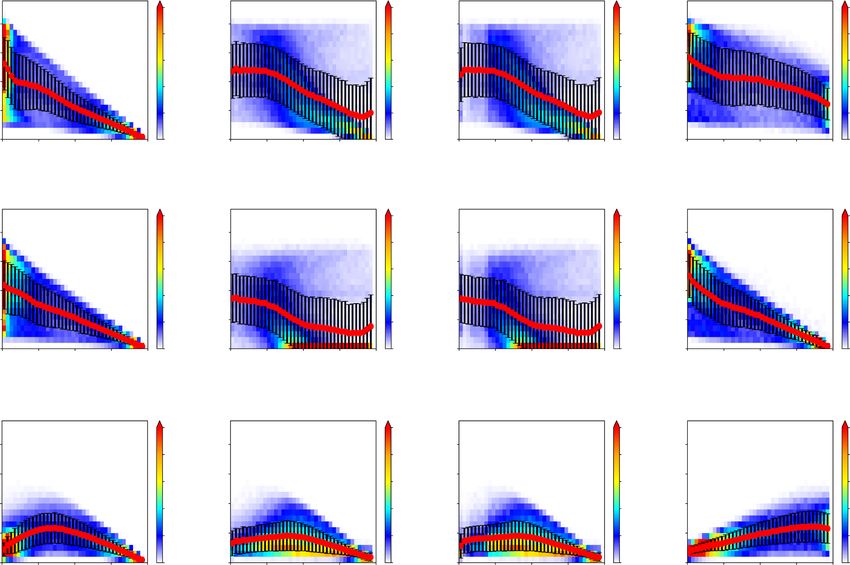
W. Liu et al. Solar Energy 215 (2021) 252–265
change the energy budget by scattering and absorbing solar radiation, Despite its utility, the simple persistence model is not capable of
which in turn depends on cloud microphysical properties (Kobayashi, forecasting solar irradiances beyond an hour as a result of neglecting the
1989; Pfister et al., 2003; Kubar et al., 2009), macroscopic properties (e. impacts of clouds and sun movement (Martín et al., 2010; Kleissl, 2013).
g., cloud fraction, cloud thickness), and multiscale structures of a cloud The smart persistence model reduces such effects somewhat, but it is
field (Shonk et al., 2010; Shonk and Hogan, 2010). On the other hand, limited to forecasting GHI only. Also, as will be shown later, the smart
radiative heating and cooling can alter the atmospheric vertical struc persistence model lumps together the different effects of cloud fraction
ture and atmospheric dynamics, changing energy redistribution of the and cloud albedo on GHI without clear differentiation.
cloud-laden atmospheric system, convective process, and cloud activ
ities (Okata et al., 2017). 2.2. Physics-informed persistence model systems
In search of a theoretical framework that connects cloud properties
with solar irradiances for retrievals and model evaluation, we (Liu et al., To further improve on the simple and smart persistence models and
2011; Xie and Liu, 2013) developed a set of equations that relates cloud explore the potentials of incorporating physics and developing a model
fraction and cloud albedo physically to reduced dimensionless quanti system that consistently forecasts not only GHI but also DNI and DHI, we
ties derived from a combination of solar irradiance components. Kumler build a hierarchy of four physics-informed persistence model systems
et al. (2019) recently presented a cloud-optical-depth-based persistence based on the theoretical framework relating solar irradiances (GHI and
model and showed improved GHI forecast over intra-hour time horizons DNI) and cloud properties (cloud fraction and cloud albedo) formulated
compared to the simple and smart persistence models. by Liu et al. (2011) and Xie and Liu (2013). This section briefly in
In this work, we first present a hierarchy of four physics-informed troduces the theoretical framework in the context of developing the
persistence models based on the theoretical formulation under forecast systems and clarifying the underlying physics; details are
different levels of physical approximations that permit forecasting not referred to the original publications.
only GHI but also its partitioning into DNI and DHI. We then evaluate Based on the concept of cloud radiative forcing widely used in
the performance of the new models, in comparison with the simple and climate studies, Liu et al. (2011) introduced the concept of relative cloud
smart persistence models, using decade-long (1998 to 2014) measure radiative forcing (RCRF) for GHI defined as
ments at the U. S. Department of Energy (DOE) Atmospheric Radiation
(3)
dn dn dn
Measurement (ARM)’s Southern Great Plains (SGP) Central Facility site. RCRF GHI = (Fclr,GHI − Fall,GHI )/Fclr,GHI
The reasons underlying the performance discrepancies are dissected as
They further showed theoretically that RCRFGHI is an approximate
well. The results shed new light on further improving observation-based
product of cloud fraction and cloud albedo. Xie and Liu (2013) extended
models to forecast GHI, DNI, and DHI.
this work by combining GHI and DNI to derive the following set of
The rest of this paper is organized as follows: the theoretical
theoretical relationships among cloud albedo (αr ), cloud fraction (f),
framework for the physics-informed persistence models is described in
GHI, and DNI given by
Section 2; the performances of the new models against the simple and
smart persistence models are given in Section 3. Further analyses ac dn
Fall,GHI dn
= Fclr,GHI − αr × f ×(F dn up 2
clr,GHI − Fall,GHI T ), (4a)
counting for the performance behavior are discussed in Section 4. The
conclusion and further work are given in Section 5. dn
Fall,DNI dn
= [1 − f + f × exp( − τ/μ0 ) ] × Fclr,DNI , (4b)
2. Theoretical framework for the physics-informed persistence τ = 2αr μ0 /[(1 − αr ) × (1 − g)], (4c)
models
up clr
∫1
where Fall,GHI is the all-sky upwelling flux; T ≈ 2 μ0 Tdd (μ0 )dμ0 is the
0
2.1. Simple and smart persistence models
transmittance of diffuse radiation of the atmosphere with μ0 represent
clr
ing the cosine of zenith angle and Tdd indicating the transmittance of
The simple and smart persistence models are well known in the solar
direct radiation that can be computed by a radiative transfer model in
forecast community; we briefly introduce here to allow the readers to
clear sky (e.g., Bird and Hulstrom, 1981); τ is the cloud optical depth; the
clearly see the connection to our new models as physics is gradually
mean value of asymmetry factor g is set as a constant 0.86. A combi
incorporated. Based on the assumptions of the persisted solar irradiance
nation of Eq. (4) yields
and clear-sky index, the simple persistence model directly projects the
historical solar irradiance to the future time steps, and the smart model αr B1
= , (5a)
decomposes the forecasting of GHI into the computation of clear-sky 1 − exp[− 2αr μ0
] B2
(1− αr )×(1− g)
index and clear-sky irradiance. Mathematically, the corresponding
forecasting equation for the simple persistence model is given by dn
Fclr,GHI − F
dn
( ) where B1 = dn up
all,GHI
2 , and B2 is the RCRF for DNI given by
dn
Fall,i dn
tf = Fall,i (t), (1) Fclr,GHI − Fall,GHI T
(5b)
dn dn dn
where Fdn represents the downward solar irradiance, the subscript ‘all’
B2 = RCRFDNI = (Fclr,DNI − F all,DNI )/Fclr,DNI
denotes the all-sky condition; tf and t are the target and historical time Eq. (5) reveals that cloud albedo is essentially a function of the ratio
such that tf = t +Δt with Δt being the forecast lead time. The subscript i B1/B2, and can be well approximated by the following piecewise
dn
can represent GHI, DNI, and DHI (note that Fall,DNI refers actually to the polynomials
vertical component of DNI here). The forecast equation for the smart
persistence model can be written as
( ) ( )
dn
Fall,GHI dn
tf = K(t) × Fclr,GHI tf , (2a)
where the subscript ‘clr’ refers to the estimated clear-sky condition,
and the clear-sky component is assessed with the method reported in
Long and Ackerman (2000) and Long and Gaustad (2004). The clear-sky
index K in Eq. (2a) is defined as
K = Fdn dn
all,GHI /Fclr,GHI (2b)
253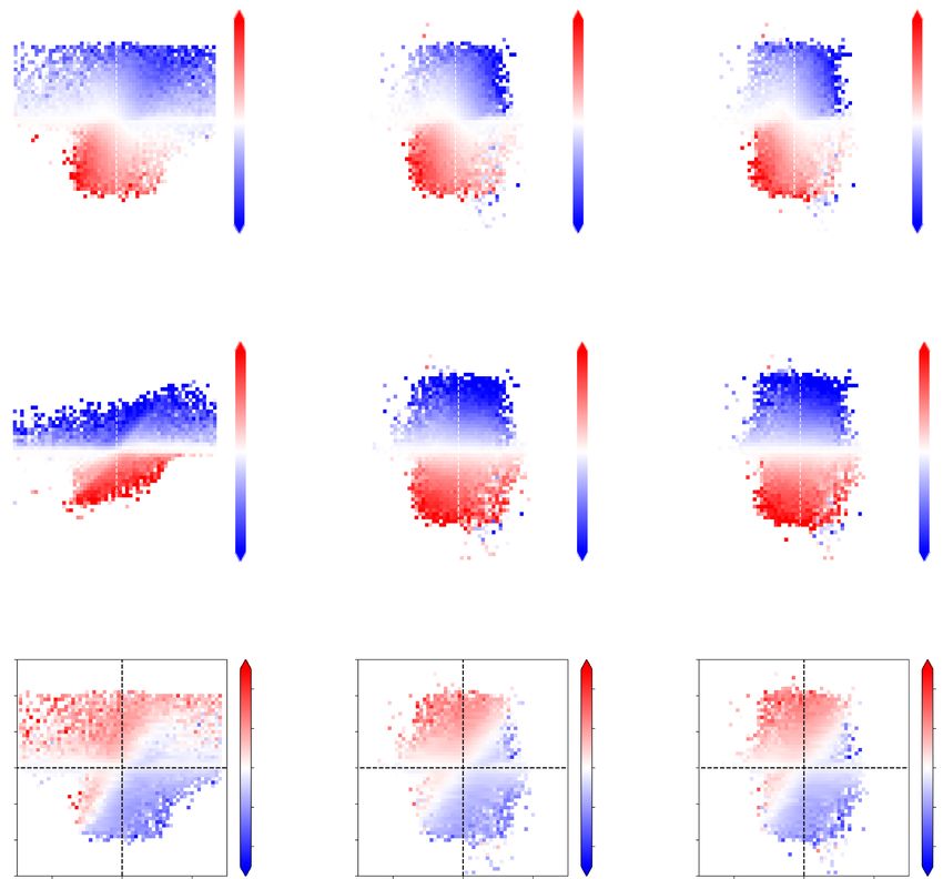
W. Liu et al. Solar Energy 215 (2021) 252–265
⎧
⎪
⎪
⎪ 0, for B1 B2 = 0 or 0.07 <
B1
< 0.07872 RCRF GHI = 1 − K. (10)
⎪
⎪ B2
⎪
⎪
⎪
⎪
⎪ √̅̅̅̅̅̅̅̅̅̅̅̅̅̅̅̅̅̅̅̅̅̅̅̅̅̅̅̅̅̅̅̅̅̅̅̅̅̅̅̅̅̅̅̅̅̅̅̅̅̅̅̅̅̅̅̅̅̅
( )2 Eq. (10) reveals that the smart persistence model is equivalent to the
⎪
⎪
⎪
⎪
⎪
B1
1 − 31.1648 + 31.1648
B1
− 49.6255
B1 RCRF-based forecast model for GHI, and thus the RCRF-based forecast
⎪
⎪
⎪
⎪ B2 B2 B2 system (hereafter RCRF-PM) can be viewed as an extension of the smart
⎪
⎪
⎪
⎪
⎪ B1 persistence model to encompass DNI and DHI in addition to GHI. Based
⎪
⎪
⎪
⎪
, for 0.07872 ≤
B2
≤ 0.11442 on Liu et al. (2011), RCRFGHI equals approximately to cloud fraction
⎪
⎪
⎪
⎪
⎨ √̅̅̅̅̅̅̅̅̅̅̅̅̅̅̅̅̅̅̅̅̅̅̅̅̅̅̅̅̅̅̅̅̅̅̅̅̅̅̅̅̅̅̅̅̅̅̅̅̅̅̅̅̅̅̅̅̅̅̅̅̅̅̅̅ times cloud albedo; thus the RCRF-PM essentially assumes persistence of
2.61224B1 − B2 + 24.2004B1 2 − 9.0098B1 B2 + B2 2 the overall cloud effects on solar irradiances.
αr = (6)
⎪
⎪
⎪
⎪
18.3622B1 − 4B2 The R-based forecast model (hereafter R-PM) takes a further step to
⎪
⎪
⎪
⎪ B1 apply the ratio of RCRFGHI and RCRFDNI to the forecast as defined in Eq.
⎪ , for 0.11442 ≤ ≤ 0.185
⎪
⎪
⎪
⎪
B2 (7), assuming the persistence of R such that
⎪
⎪
⎪
⎪ B1 B1 ( ) [ ( )* ] ( )
⎪
⎪
⎪ 0.89412 + 0.02519 , for 0.185 < ≤ 0.23792 dn
Fall,GHI tf = 1 − R(t) × RCRF DNI tf dn
× Fclr,GHI tf , (11a)
⎪
⎪ B2 B2
⎪
⎪
⎪
⎪ ( ) [ ( )* ] ( )
⎪
⎪
⎪
⎪
⎪ B1 B1
dn
Fall,DNI dn
tf = 1 − RCRF GHI tf /R(t) × Fclr,DNI tf , (11b)
⎪
⎩ for 0.23792 < ≤ 1.0
B2 B2
where the variable with a superscript * in Eqs. (11a) and (11b) is esti
Once αr is determined, cloud fraction f can be estimated by Eq. (4a). mated with
Two points are worth highlighting for this study. First, B1 can be ∑t j
up
approximated by RCRFGHI because the term Fall,GHI T2 is much smaller
( ) j=0 (1 − a) V(t − j)
V tf = ∑t j , (12)
than Fclr,GHI
dn
in the B1 denominator (5%~7%) and thus can be ignored. j=0 (1 − a)
Thus, the theoretical formulation reveals that cloud albedo is essentially
where V denotes the variable to be estimated; j denotes the time step in
a function of the ratio of the RCRF for GHI and DHI defined as
the past 5 time steps; a is a smoothing parameter set as 1/3 for the
R = RCRFGHI /RCRFDNI . (7) exponential weighted moving average over 5-time steps.
The 4th level forecast system has two models. One assumes the
In other words, the RCRF ratio R is essentially determined by cloud
persistence of cloud albedo (cloud albedo-based forecast model and
albedo. Second, with the approximation of B1 = RCRFGHI, Eq. (4a) is
denoted by CA-PM hereafter), and the forecast equation is given by
reduced to
( ) ( )
dn
Fall,GHI tf = [1 − αr (t) × f (tf )* ] × Fclr,GHI
dn
tf (13a)
dn
Fall,GHI = (1− αr × f ) × F dn
clr,GHI (8a)
( ) ( )* ( )* ( )/ ( )
or f = B1 /ar ≈ RCRF GHI /ar ≈ RCRF DNI . (8b)
dn
Fall,DNI dn
tf = [1− f tf + f tf × exp[− τ tf μ0 (tf )] × Fclr,DNI tf (13b)
Equation (8b) reveals that RCRFDNI is essentially determined by ( ) 2αr (t)μ0 (tf )
cloud fraction. It is noteworthy that Yang et al. (2012) showed an τ tf = (13c)
(1 − αr (t)) × (1 − 0.86)
empirical relationship between cloud fraction and DNI clear-sky index
defined as the ratio of all-sky DNI to the clear-sky DNI, providing where the variable marked with a superscript * also can be approxi
observational support for the theoretical Eq. (8a). mated by Eq. (12).
According to the above theoretical analysis, we can build a hierarchy The other 4th level forecast model assumes the persistence of cloud
of persistence model systems to forecast GHI, DNI, and DHI, with fraction (cloud fraction-based forecast system and denoted by CF-PM
different levels of incorporating physics as summarized in Table 1. The hereafter), and the forecast equation is given by
corresponding forecast systems are described next. ( ) [ ( )* ] ( )
The 1st level persistent model directly assumes the persistence of
dn
Fall,GHI dn
tf = 1 − αr tf × f (t) × Fclr,GHI tf , (14a)
GHI, DNI and GHI; an example is the well-known simple persistence ( ) ( )/ ( )
model for GHI. The 2nd level forecast model assumes the persistence of
dn
Fall,DNI dn
tf = [1 − f (t) + f (t) × exp[(− τ tf μ0 (tf )] × Fclr,DNI tf , (14b)
clear-sky index or RCRFs (RCRF-based persistence model hereafter), and
( )*
the forecasting equation is given by ( ) 2αr tf μ0 (tf )
τ tf = ( ) (14c)
dn
Fall,i
( ) dn
tf = [1 − RCRF i (t) ] × Fclr,i
( )
tf , (9) 1 − αr (tf )* × (1 − 0.86)
Note that the prediction for DNI and DHI of all the new forecast
where the subscript i denotes GHI, DNI, and DHI. It can be readily shown systems are derived by
that RCRFGHI has a linear relationship with K given by
dn
Fall,DNI = FDNI /μ0 , (15a)
( ) ( ) ( )
dn
Fall,DHI dn
tf = Fall,GHI dn
tf − Fall,DNI tf , (15b)
Table 1
A summary of cloud-radiation relationships at different levels of approximation. where the cosine of the solar zenith angle μ0 can be calculated with the
Hierarchy Persistent Cloud physics incorporated method reported by Reda and Andreas (2004); the solar zenith angle
level predictor from the dataset is used in this study.
1st level Fdn
all,GHI , Fall,DNI ,
dn No direct cloud physics
Fdn
all,DHI
3. Forecast and evaluation
2nd level K or RCRFs Overall cloud effects
3rd level R Approximate separation of radiative effects from 3.1. Measurement data
cloud albedo and cloud fraction
4th level αr,f Clear separation of radiative effects from cloud
We have tested the hierarchy of new forecast systems with the
albedo and cloud fraction
254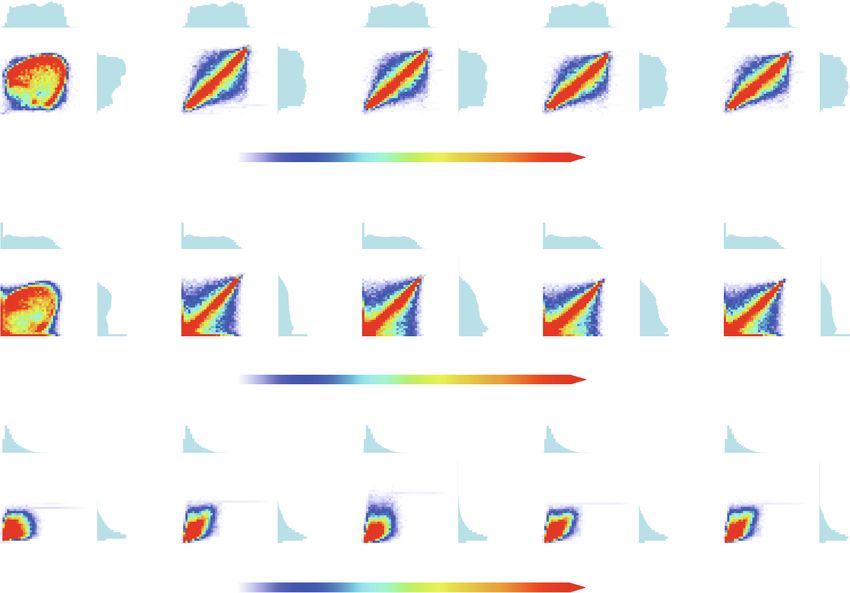
W. Liu et al. Solar Energy 215 (2021) 252–265
decade-long (from 1998 to 2014) and quality-controlled measurements the simple (Ssimple) or smart persistence model (SRCRF). Note that RCRF-
of GHI, DNI, and DHI with the 15-minute resolution at the U. S. DOE PM is equivalent to the smart persistence model for GHI, and can be
ARM SGP Central Facility site. The site is also chosen for its availability regarded as the extension of the smart persistence model for DNI and
of co-located measurements of detailed data on atmospheric processes DHI. Positive and negative values of S indicate that the new model im
relevant to clouds and solar radiation (www.arm.gov). The clear-sky proves and degrades the forecast relative to the reference persistence
components are assessed based on the method proposed by Long and model, respectively. The magnitude of the skill score quantifies the de
Ackerman (2000) and Long and Gaustad (2004). gree of forecast improvement or degradation as compared to the refer
ence persistence model. Fig. 2 shows the PE skill scores as a function of
3.2. Overall performance lead time for different models in forecasting GHI (a,d), DNI (b,e) and
DHI (c, f) relative to the simple and smart (RCRF) persistence model.
For convenience of discussion, various quantities assumed to be Several points are noteworthy. First, for GHI, all the new models
persistent (e.g., RCRFs, R, cloud albedo, and cloud fraction) are gener outperform the simple and smart persistence model at all the lead times
ically referred to as cloud predictors. A common criterion 1 W⋅m− 2 < examined (from 15 min to 6 h), and the improvement increases with
Fall(tf) < 1361 W⋅m− 2 (mean solar constant) (Kopp and Lean, 2011; increasing lead times. CF-PM has the best performance with improve
Kopp, G., 2014) is used to determine the valid data for the models. As ment up to 68% and 29% at 6-hour lead time compared to the simple
indicated in Table 2, the maximum percentages of the outliers at all the and smart persistence model, respectively. It is noteworthy that the
lead times examined, are less than 0.47%, 8.8% and 5.2% for GHI, DNI difference between CA-PM and CF-PM is negligible, and both models
and DHI, respectively. These results suggest a minimal influence of the have slightly better performance than the third-level model, R-PM. The
excluded outliers on the evaluation and subsequent analysis. The higher results clearly demonstrate the enhancement of the skill scores in fore
percentage for DNI and R-PM may result from the operation of division casting GHI resulting from incorporating physics into the forecast
and approximations involved (Eqs. (11)–(14)). To further assure the models at different levels of the hierarchy, and the model at the higher
consistency of comparison across the different models and radiative level tends to have better performance. Second, for DNI, the improve
components, the same set of data are used for performance evaluation ments of the third and fourth level models increase with increasing lead
that produce valid predictions of GHI, DNI and DHI in all the models. times similar to GHI, and they all outperform the simple persistence
Fig. 1 compares the overall performance of different forecast systems model and RCRF-PM from 0.75-hour and 1.25-hour lead time, respec
in terms of percentage error (PE) defined as the root mean squared error tively. CA-PM performs the best, with improvements up to 47% and 15%
normalized by the mean measurement at lead times from 15 min up to 6 relative to the simple model and RCRF-PM. It is noted that the perfor
h. A few points are evident. First, for GHI, although the simple persis mance of R-PM is worse than the simple persistence model and RCRF-PM
tence model has a comparable PE at lead times less than 1 h, all the in forecasting DNI (s < 0) at lead times less than 0.75 and 1.25 h,
physics-informed persistence models outperform the simple persistence respectively. Third, for DHI, the improvement starts from 1-hour lead
model at all lead times, with significant improvements especially over time for all but R-PM. Despite the general increase of the skill score with
longer forecasting horizons beyond 1 h. These results are consistent with increasing lead times as well, the improvements are less than 30% for
the previous studies on the GHI forecast (Martín et al., 2010; Kleissl, DHI based on Ssimple, smaller than those for GHI and DNI forecasts, which
2013). Second, all the other physics-informed forecast systems have is likely related to the error propagation/enhancement, since it is
smaller PEs than the smart persistence model (note the equivalence of essentially calculated as a difference between forecasted GHI and DNI.
RCRF-PM for forecasting GHI with the smart persistence model) beyond R-PM starts to forecast DHI better than the simple persistence model at a
1.25 h, indicating better accuracies of the new forecast systems in later lead time of 3 h, and it is postponed to 4 h regarding SRCRF. The
forecasting GHI. The performances of the fourth level models, CF-PM relatively poor performance of R-PM for DNI and DHI might be related
and CA-PM, are even better than that of the third level R-PM in fore to the above-mentioned approximations involved in deriving the R ratio.
casting GHI despite the minor differences among those three models. Another metric to gauge forecast models lies in the improvements in
Third, the physics-informed persistence models successfully partition the forecast lead time given a reference forecast accuracy. It is recog
GHI into DNI and DHI with forecasting accuracies comparable to the nized that the simple persistence models generally have acceptable
conventional smart persistence model for GHI. Generally, CF-PM has the forecasting accuracy within the 1-hour forecasting horizon (Diagne
best performance in forecasting GHI, but CA-PM outperforms the other et al., 2013), which is also shown in Fig. 1. Thus, we choose the PEs of
models in predicting DNI and DHI at lead times longer than 1 h. Finally, simple persistence models at the lead time of 1 h as the reference to
the forecast accuracy for GHI is generally better than those for DNI and identify the lead time of the other models with similar PEs and quantify
DHI at the same lead time. the improvement in forecast lead time over the simple persistence
To better illustrate the quantitative improvement over the simple model. The results are summarized in Table 3. Relative to the simple
and smart persistence model, we calculate the PE skill score (S) for all persistence model, RCRF-PM, R-PM, CA-PM and CF-PM extend the lead
the models with lead times from 15 min to 6 h. The PE skill score is times from 3 h up to 6 h (longest lead time examined) for GHI; the
defined as (Yang et al., 2020) corresponding extensions for DNI are 1.75 h, 2 h, 2.5 h, and 2 h,
( ) respectively. The improvements in lead time for DHI are not as signifi
sreference = 1 −
PEmodel
*100%, (16) cant as the other two components with all being smaller than 1.25 h.
PEreference Similarly, Table 4 lists the improvements in forecast lead times of the
third and fourth level models over the smart (RCRF) persistence model.
where the subscript “model” denotes one of the new models, and the To further examine the error components determining PE, we modify
subscript “reference” indicates that the reference persistence model is the Taylor diagram (Taylor, 2001) to show the individual error com
ponents (correlation coefficient r between the measurement and fore
Table 2 cast, normalized standard deviation σ = σpre /σ obs (σ pre andσobs represent
Maximum percentage (%) of the outliers for individual models. the standard deviation of model and measurement, respectively), and
Model GHI DNI DHI the centered root-mean-squared error (CRMSE) (1 + σ 2 − 2σ *r) at all
Simple 0.0029 2.4 0.0012 lead times (Fig. 3). The shorter the distance between each point and the
RCRF-PM (smart) 0.019 2.2 0.048 reference point ‘Ref’, the smaller the CRMSE. The modification lies in
R-PM 0.47 8.8 5.2 the additional representation of the magnitude of mean bias between the
CA-PM 0.055 0.62 0.14 measured and predicted solar irradiances by different colors and lead
CF-PM 0.055 2.7 0.11
255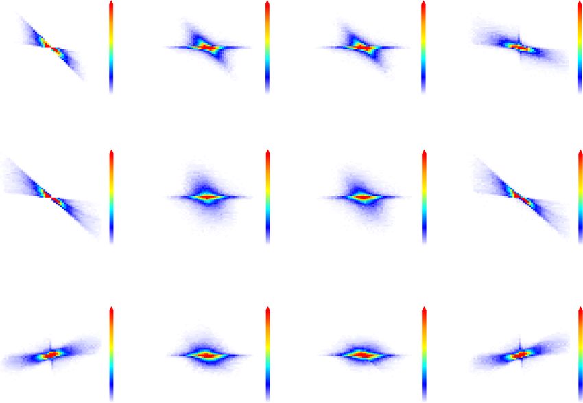
W. Liu et al. Solar Energy 215 (2021) 252–265
Fig. 1. Overall performance of all forecast systems as a function of forecast lead time.
Fig. 2. PE skill score as a function of lead time for different models. Ssimple and SRCRF mean the PE skill scores are referenced by the simple and smart (and RCRF)
persistence models, respectively.
Table 3 Table 4
Improvement in forecast lead times of the new models over simple persistence Improvement in forecast lead times of the new models over smart (RCRF)
model. persistence model.
RCRF-PM R-PM CA-PM CF-PM R-PM CA-PM CF-PM
GHI 3h 5.5 h 6h 6h GHI 1.5 h 1.5 h 1.75 h
DNI 1.75 h 2h 2.5 h 2h DNI 1h 1.25 h 1.25 h
DHI 1.25 h 0h 1.25 h 1.25 h DHI 1h 1h 1h
times by different symbol sizes. With all the error components of PE various models. Some features are noteworthy. First, model perfor
represented, the modified Taylor diagram helps to determine the indi mance gradually degrades with an increasing CRMSE as the lead time
vidual factors resulting in the differences in the performances among increases. With the exception of RCRF-PM, the increase of CRMSE is
256
W. Liu et al. Solar Energy 215 (2021) 252–265 Fig. 3. Taylor diagram illustrating the model performances at all lead times. The top, middle, and bottom rows are for GHI, DNI, and DHI; different columns are for different models; different symbol sizes and colors are for various lead times and the mean absolute errors between the measured and forecasted solar irradiances, respectively. The radial distance from the origin is proportional to the normalized standard deviation. The centered RMSE (green dotted lines) between the forecast and observation field is proportional to their distance apart. The blue dotted lines indicate the correlation coefficient between the forecast and reference field. Note the error bar for the simple persistence model is not the same as the other models. (For interpretation of the references to color in this figure legend, the reader is referred to the web version of this article.) mainly caused by the decrease of the correlation coefficient, since the observations and forecasts can be compared, and more detailed joint variation of the normalized standard deviation with lead time is mini distribution can be evaluated. Fig. 4 further shows an example of mal. Similarly, the smaller CRMSE for GHI compared to DNI and DHI comparing different forecasts at the lead time of 3 h against the corre results mainly from the higher correlation as well. As for RCRF-PM, a sponding measurements. As can be seen that the scatters of the simple distinction from the other models is embodied in the increasing persistence model are much broader than the other models for all the normalized standard deviation with lead time, which is responsible for solar radiative components. In general, the fourth-level based models, the growing CRMSE as well. Second, at the lead times with positive CA-PM and CF-PM, outperform the other models with the data points Ssimple as shown in Fig. 2, the physics-informed forecast systems centering around the perfect one-to-one line. Without referencing the outperform the simple persistence models mainly due to smaller mean modified Taylor diagram or PE, it is difficult to determine which model biases and higher correlation. At the lead times with positive Ssmart, the is the best due to the visually similar scatters between these two. The physics-informed forecast systems have better performance mainly second and third level-based models, RCRF-PM and R-PM, tend to resulting from smaller mean biases and smaller standard deviation overestimate the high-value irradiances, with the high occurrence fre rather than higher correlation; the correlation coefficients are similar for quency zone shifting upward from the one-to-one line. Moreover, the RCRF-PM and the other physics-informed models. Nevertheless, at the histograms display the marginal distributions of measurement (on the lead times with negative S, relative to the simple or smart persistence top) and forecast (on the right). For clarity, the forecasted and measured model, the worse performance of the physics-informed models stems marginal cumulative distributions are further compared in Fig. 5 for GHI from a lower correlation and/or a higher mean bias. For example, R-PM (a), DNI (b), and DHI (c). Visually, the new persistence models can well has negative SRCRF at the lead times less than 1.25 h and 4 h for DNI and capture the observed GHI distribution. A larger discrepancy between the DHI forecasts, respectively, and the Taylor diagram suggests that the forecasted and observed marginal distributions exists under low DNI and lower correlation coefficient and larger mean bias are responsible for the DHI conditions (

W. Liu et al.                                                                                                                           Solar Energy 215 (2021) 252–265

Fig. 4. Joint and marginal distributions of the predicted and observed solar irradiances at the lead time of 3 h. Different columns are for different models as marked
on the center top of the plots in the top row. The top, middle and bottom rows are for GHI, DNI, and DHI, respectively; the plots in the same row share the same
colorbar displayed at the end; the black dashed line is the one-to-one line; the top and right marginal distributions are for observations and forecasts, respectively.

Fig. 5. Comparison between the observed marginal cumulative distributions and those forecasted by the different models. The radiative components are given on top
of plots.

W⋅m− 2).                                                                               various solar irradiances, the fourth-level models (CF-PM and CA-PM)
   Together, the analyses demonstrate that the new physics-informed                    perform the best. This makes physical sense considering that the third-
forecast systems are capable of predicting GHI, DNI, and DHI and                       level R-model framework is an approximation of the fourth-level
outperform the simple and smart persistence model, especially over                     framework, the second-level RCRF system considers the overall cloud
longer time horizons (>1.25 h) by reducing measurements of GHI and                     radiative effects without separation, and the first level models consider
DNI into dimensionless cloud predictors that are related to different                  solar radiation directly without explicitly considering any cloud effects.
cloud properties. Furthermore, regardless of the detailed differences for

                                                                                 258
W. Liu et al. Solar Energy 215 (2021) 252–265
4. Further analysis
V(t + Δt) − V(t)
ε=| | × 100%, (17)
V(t)
As qualitatively illustrated in Fig. 6, large forecast errors are often
related to the cloudy episodes with a dramatic temporal variation of
where V denotes the variable in question, t is the time, andΔt is the time
cloud properties, suggesting the possible linkage between the variability
difference between the steps (hereafter referred to interval time for
of cloud property and model performance. This section further explores
convenience). The use of the relative variability permits the comparison
the quantitative relationships between them.
of quantities with different physical units; taking the absolute value
To quantify the temporal variation, we introduce the magnitude of
allows us to focus on the magnitude of the variation to better show the
the relative variability (ε) defined as
trend of the statistical meanε with interval time without being influ
enced by the sign. Fig. 7 shows an example of the temporal variations of
ε for solar irradiances and cloud properties at the interval time of 3 h in
Fig. 6. A case on 09/07/2002; (a) ~ (e) show the temporal variation of GHI, DNI, DHI, cloud properties, and ground-based-observed cloud fraction; (f) ~ (h) are the
forecasted errors from all the systems for GHI, DNI, and DHI at the lead time of 2 h. Four sky images from the top left to the bottom right correspond to the local time
10:00, 12:00, 14:00, and 16:00, respectively.
259W. Liu et al. Solar Energy 215 (2021) 252–265
Fig. 7. Temporal variation of the magnitude of relative variability ε for radiative components and cloud predictors at the interval time of 3 h. The red line represents
the mean ε. (For interpretation of the references to color in this figure legend, the reader is referred to the web version of this article.)
2014. The mean ε for GHI is much smaller than that of DNI, indicating a the mean ε at the same lead time does not affect the PE significantly,
gentle variation in GHI from t to t + Δt, which is potentially associated both of which possibly imply other factors influencing the model per
with the best performance among three radiative components by using formance in addition to the temporal variability. Moreover, though a
one type model to forecast GHI (Figs. 1–3). Even though the smallest ε in smaller ε in GHI than the other cloud predictors, the worst performance
DHI, it is derived in an indirect way with the forecast accuracy being of the simple model could be possibly explained as by the physical un
both affected by the signature of GHI and DNI, leading to worse per derstanding that this predictor does not embody a specific type of cloud
formance in DHI compared to GHI. Furthermore, the fourth-level- influence, but the irradiance itself. These findings highlight the linkages
properties (cloud fraction and cloud albedo) have smaller mean εthan among solar radiation changes, temporal variability of cloud properties,
the other level ones (R, RCRFs), supporting that the fourth-level-model and model performances, and also suggest the minimal ε principle in
systems outperform the other models in predicting individual radia general for choosing the cloud predictor among different hierarchy
tive components. To illustrate the connections between temporal vari levels to build the corresponding forecast system.
ability and model performance extended to all interval times examined The increasing mean ε with the increasing interval time essentially
and the long-term periods, Fig. 8 relates the mean ε (from 1998 ~ 2014) indicates the growing forecast errors with lead time, which makes the
of the cloud predictor with the PE from the corresponding predictor- assumption of the persistence of the key predictors used in the model is
based model when the lead time is equal to the interval time, showing more questionable for long lead times. Based on the assumptions, a
that PE positively correlates with the mean ε for all the models, and both larger error between the actual and the assumed persistent cloud pre
generally increase with lead time. In general, the smaller mean ε asso dictor (RCRF, R, cloud albedo, and cloud fraction) is likely translated
ciated with better performance in GHI and the fourth-level-based sys into a larger error in the solar irradiance forecast (see the corresponding
tems agrees well with Fig. 7; however, the minimum mean ε in cloud forecast equations in Section 2). To confirm this, Fig. 9 shows the rela
albedo only contributes the least to PE for DNI and DHI, but not for GHI, tionship of the errors between cloud predictors and GHI (top panel), DNI
and meantime model performances are relatively independent of the (middle panel), and DHI (low panel) at the lead time of 2 h. Also shown
mean ε among R-PM, CF-PM and CA-PM, since the discrepancy between are the PEs of the models. Several points are noteworthy. First, with
Fig. 8. Percent error (PE) as a function of the mean ε for the cloud predictors at all the lead times.
260W. Liu et al. Solar Energy 215 (2021) 252–265
Occurrence
Occurrence
Occurrence
Occurrence
Occurrence
Occurrence
Occurrence
Occurrence
Occurrence
Occurrence
Occurrence
Occurrence
Fig. 9. Relationships between the errors in cloud predictors and solar irradiances with the corresponding PEs at the lead time of 2 h. The top, middle, and bottom
rows are for GHI, DNI, and DHI, respectively; different columns represent different models as marked on the top in the first row.
three exceptions. All the error correlations are negative for GHI and DNI, radiation. To illustrate the point, Fig. 10 (a) ~ (c) show the slope (m) of
suggesting that underestimated (overestimated) cloud properties (e..g, the linear-fitting equation between the error in the cloud predictor (x)
cloud fraction and cloud albedo) lead to overestimated (underestimated) and the error in the solar irradiance (y) with the expression of y = mx, m
solar irradiances. One exception is the relationship between the error in is used as an indicator of propagation strength; the intercept is set as zero
cloud fraction (and RCRFDNI, RCRFDNI≈f) and the error in forecasted to eliminate its influence on the results when comparing different m at
DHI, which is positive, suggesting that an underestimated (over various lead times. Fig. 10 (e) ~ (f) show the correlation coefficient (r)
estimated) cloud fraction (and RCRFDNI) leads to underestimated between x and y. The negative m and r for all the physical models in GHI
(overestimated) DHI. These results seem consistent with the physical and DNI forecasts further confirm that the error in solar radiation
understanding that clouds normally enhance DHI, but reduce DNI and negatively correlates with the error in cloud predictor at all the lead
GHI. The other two exceptions are the relationships of the error in the times as supplementary to Fig. 9. Meanwhile, regardless of the details on
forecasted DNI to the errors in R and cloud albedo, both of which are the variation in m and r with lead time, a consistent ranking order be
largely independent. This error independence seems to accord with the tween them among different cloud predictors also indicates that the
physical understanding that DNI is determined primarily by cloud magnitude of m can roughly represent the correlation r between pre
fraction (Yang et al., 2012; Xie and Liu, 2013). Second, the details of the dictor error (x) and solar radiation error (y), and vice versa. The mag
error relationships vary among different cloud predictors and radiative nitudes in m and r vary among cloud predictors, manifesting their
components. For example, on one hand, for individual cloud predictor, different propagation strengths from predictor error to the solar irradi
the error contributes a wider variation range to the error in DNI ance error and thus regulate the model performance by its integration
compared to GHI; on the other hand, for the same radiative component, with the error in cloud predictor. For example, the relatively larger error
the error in cloud albedo contributes the least to the error in DNI as well in RCRFs (Fig. 8) and the stronger propagation strength both contribute
as in DHI with the smallest PE compared to the other three cloud pre to a large radiation error (y) degrading performance with the largest PE
dictors (RCRF, R and cloud fraction) but not shown in the GHI forecast. in RCRF-PM except for the simple model. Conversely, a plausible reason
All these results indicate the different sensitivities of the radiation error for the best performance of CA-PM in DNI and DHI forecasts is due to the
to the cloud predictor error. smallest error (Fig. 8) in cloud albedo as well as the relatively weaker
The sensitivity of the radiation error to the cloud preditor error propagation strength (Fig. 10). Moreover, the combined effects of the
basically refers to the propagation strength from the predictor error to propagation strength (or correlation) and the error in cloud predictor
the solar irradiance error. As can be seen from Fig. 9, cloud albedo and R are possibly responsible for the independent relationship of PE with the
have relatively weaker propagation strength due to the visually inde mean ε among R-PM, CA-PM and CF-PM as shown in Fig. 8, the differ
pendent relationship between the errors in cloud predictor and ence in the ranking order between the mean ε and correlation among R,
261W. Liu et al. Solar Energy 215 (2021) 252–265
Fig. 10. (a) ~ (c) shows the slope (m) of the linear regression equation, y = mx, as a function of lead time, where y and x, respectively, denote the error of the solar
irradiance and cloud predictor for each model. (d) ~ (f) show the correlation coefficient (r) between x and y as a function of lead time.
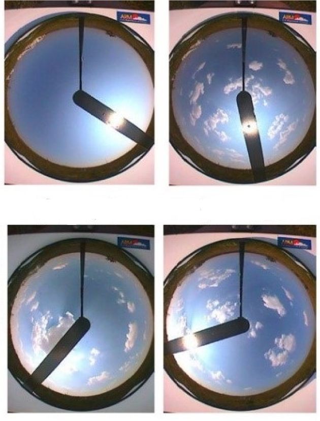
cloud albedo and cloud fraction makes it possible to result in similar complicated relationships; it increases with cloud fraction, but it in
model performance. creases with RCRFGHI, R and cloud albedo only when their values are less
The preceding analysis discussed the relationship between the error than 0.4, and then DHI decreases with them as they further increase.
in the key cloud predictor and the model performance without differ These results seem consistent with the physical understanding that
entiating the impact of the potential error from the other assumed var clouds normally enhance DHI but reduce DNI and GHI, and that also
iables introduced by applying the exponential technique (i.e., assumed accounts for the underestimated cloud predictors causing an over
RCRFs in R-PM, assumed cloud fraction in CA-PM, and assumed cloud estimated GHI and DNI as well as underestimated cloud fraction leading
albedo in CF-AM). The joint impact of the errors from both variables on to an underestimated DHI, as shown in Fig. 9.
the solar radiation error is further investigated given by Fig. 11. Note These findings also help explain the performance among different
that the x-axis denotes R or cloud albedo due to the relationship of R≈αr radiative components and different models. It is clear that the con
for better comparison regardless of the assumption technique (persis trasting dependences of DNI and DHI on cloud fraction somewhat cancel
tence or exponential moving average) applied to cloud predictors. each other as the cloud fraction varies, which only leads to a slightly
Different patterns are shown for various radiative components. In GHI decreasing trend in GHI with cloud fraction (first row, last column in
forecast, large radiation errors mainly occur in the first and third Fig. 11) as GHI theoretically is the sum of DHI and the vertical
quadrant with either negative or positive error in two cloud predictors. component of DNI. The contrasting dependencies of DNI and DHI on the
The underestimated (overestimated) solar radiations mainly occur when other predictors (RCRF, R, and cloud albedo), however, occur only when
the error in cloud fraction or RCRFGHI is greater (less) than 0, but the the value of the cloud predictor is less than 0.4; beyond that, obvious
variation in the sign of the cloud albedo error does not cause a signifi descending trends on GHI are shown because of the reductions both on
cant variation in the DNI error. In DHI forecast, the overestimation and DNI and DHI with RCRF, R and cloud albedo. The feature infers that GHI
underestimation in DHI are separated by a split line across the first and has a gentle variation with the increasing cloud fraction causing a
third quadrant with an angle to the x-axis around 45◦ , the methodology smaller error in GHI when using CF-PM to make a forecast compared to
in deriving DHI makes the relationship complicated and not straight the other models. Conversely, DNI is determined primarily by cloud
forward. That DNI error mainly determined by the cloud fraction error is fraction, and a small error in cloud fraction will introduce a noticeable
consistent with the results shown by Figs. 9 and 10, and agrees with error in DNI. However, DNI is relatively independent of cloud albedo or
Yang et al. (2012). R, which not only supports the above-mentioned largely independent
To further investigate the physical reasons underlying the model relationships of the error in forecasted DNI to the errors of R and cloud
behaviors, Fig. 12 shows the relationships between solar irradiances and albedo, but also indicates a better performance on DNI when R-PM and
cloud predictors based on the all measurements examined. Both GHI CA-PM are used. Despite the similar relationships between solar radia
(top panel) and DNI (middle panel) irradiances decrease with increasing tion and cloud albedo and R, the smaller error in cloud albedo than in R
values of the cloud predictors. DHI (lower panel) exhibits more at the same lead time (Fig. 9, Fig. 11) seems to account for the better
262W. Liu et al. Solar Energy 215 (2021) 252–265
Fig. 11. Relationships between the errors in two estimated cloud predictors in R-PM (first column), CA-PM (second column) and CF-PM (third column) at lead time
of 3 h. The colorbar shows the error in solar irradiance; different rows are for different radiative components.
performance in CA-PM than R-PM in forecasting DNI. detailed differences for various solar components, the fourth-level
forecast systems (CA-PM and CF-PM) have the overall best perfor
5. Concluding remarks mance among the models. Further analysis shows that model perfor
mance is related to the temporal variability of the cloud predictor
A hierarchy of four new physics-informed persistence models is assumed to be persistent: a larger variability between the actual and the
presented to improve the ability to forecast both GHI and its partitioning assumed persistent cloud predictor will generally translate into a larger
into DNI and DHI by incorporating clear physics into the persistence error in the solar irradiance forecast.
models based on the theoretical framework that connected solar irra The results clearly demonstrate the importance and utility of incor
diances with cloud properties (Liu et al., 2011; Xie and Liu, 2013). The porating physics into developing observation-based forecast models. A
decade-long measurements at the ARM SGP Central Facility site are few points are noteworthy. First, this study is primarily focused on the
utilized to evaluate the performance of these models and compared overall cloud influences without the separation of different cloud types.
them with the commonly used simple and smart persistence models. An In the future, it is desirable to test the forecast systems under different
in-depth analysis is conducted as well to assess the model performance cloud types. Also desirable is to evaluate the models in different climate
and associate it with specific cloud predictors. zones and locations. Second, in this study, the prediction for DHI is
Our results show that the new physics-informed models outperform obtained by use of the equality DHI = GHI-DNI*μ0, and thus the errors
the simple and smart persistence models and improve the forecasting from GHI and DNI will both affect predicting DHI irradiance. A direct
accuracy of GHI, DNI, and DHI at long lead times (>1.25 h). Generally, method is more desirable. Third, as the first proof of concept, this study
CF-PM demonstrates the best performance in predicting GHI, and CA- focuses primarily on the persistence models, advanced approaches (e.g.,
PM is the best forecast system for DNI and DHI forecast based on the machine learning) in time-series forecasting merits exploration in the
overall performance evaluated by the percent error. Regardless of the future. Last, the theoretical framework presented in Liu et al. (2011) and
263W. Liu et al. Solar Energy 215 (2021) 252–265
Occurrence
Occurrence
Occurrence
Occurrence
Occurrence
Occurrence
Occurrence
Occurrence
Occurrence
Occurrence
Occurrence
Occurrence
Fig. 12. Relationships between cloud predictors and solar irradiances The top, middle, and bottom rows are for GHI, DNI, and DHI, respectively; different columns
show the relationships between solar irradiances with RCRF, R, cloud albedo, and cloud fraction, respectively. The red line with the black error bar indicates the
mean ± standard deviation of solar irradiance. The plots are based on all the measurements examined and the color bar shows the occurrence frequency of cor
responding data points. (For interpretation of the references to color in this figure legend, the reader is referred to the web version of this article.)
Xie and Liu (2013) have inherent assumptions that may not hold for Energy under Contract No. DE-AC36-08GO28308. The views expressed
ambient clouds. For example, the homogeneous cloud assumption in the article do not necessarily represent the views of the Department of
cannot accurately represent 3-D radiative transfer in some clouds (e.g., Energy or the U.S. Government. The U.S. Government retains and the
deep convective clouds). Careful use of this method in such specific publisher, by accepting the article for publication, acknowledges that
scenarios is needed. The impacts of the overlapped clouds, aerosols and the U.S. Government retains a nonexclusive, paid-up, irrevocable,
the 3-D cloud effect are not yet considered in our model. The model is worldwide license to publish or reproduce the published form of this
expected to be more accurate when considering these factors, and work, or allow others to do so, for U.S. Government purposes.
associated works in the future are needed to be explored.
References
Declaration of Competing Interest
Bailek, N., Bouchouicha, K., Al-Mostafa, Z., El-Shimy, M., Aoun, N., Slimani, A., Al-
Shehri, S., 2018. A new empirical model for forecasting the diffuse solar radiation
The authors declare that they have no known competing financial over Sahara in the Algerian Big South. Renewable Energy 117, 530–537.
interests or personal relationships that could have appeared to influence Beltran, H., Perez, E., Aparicio, N., Rodríguez, P., 2012. Daily solar energy estimation for
the work reported in this paper. minimizing energy storage requirements in PV power plants. IEEE Trans. Sustainable
Energy 4 (2), 474–481.
Bird, R.E., Hulstrom, R.L., 1981. Simplified clear sky model for direct and diffuse
Acknowledgements insolation on horizontal surfaces (No. SERI/TR-642-761). Solar Energy Research
Inst., Golden, CO (USA).
Chu, Y., Li, M., Pedro, H.T., Coimbra, C.F., 2015. Real-time prediction intervals for intra-
The authors are grateful to Dr. Dazhi Yang Singapore at the Institute hour DNI forecasts. Renewable Energy 83, 234–244.
of Manufacturing Technology, and anonymous reviewers for their Diagne, M., David, M., Lauret, P., Boland, J., Schmutz, N., 2013. Review of solar
valuable comments. The data are downloaded from the DOE ARM irradiance forecasting methods and a proposition for small-scale insular grids.
Renew. Sustain. Energy Rev. 27, 65–76.
website (www.arm.gov). The work is supported by the U.S. Department
Inman, R.H., Pedro, H.T., Coimbra, C.F., 2013. Solar forecasting methods for renewable
of Energy’s Office of Energy Efficiency and Renewable Energy (EERE) energy integration. Prog. Energy Combust. Sci. 39 (6), 535–576.
under Solar Energy Technologies Office (SETO) [grant number 33504] Kleissl, J., 2013. Solar energy forecasting and resource assessment. Academic Press.
Kobayashi, T., 1989. Radiative properties of finite cloud fields over a reflecting surface.
and Atmospheric System Research (ASR). The Brookhaven National
J. Atmos. Sci. 46 (14), 2208–2214.
Laboratory is operated by the Brookhaven Science Associates, LLC Kopp, G., 2014. An assessment of the solar irradiance record for climate studies. J. Space
(BSA), for the U.S. Department of Energy under Contract No. DE- Weather Space Clim. 4, A14. https://doi.org/10.1051/swsc/2014012.
SC0012704. The National Renewable Energy Laboratory is operated
by Alliance for Sustainable Energy, LLC, for the U.S. Department of
264W. Liu et al. Solar Energy 215 (2021) 252–265
Kopp, G., Lean, J.L., 2011. A new, lower value of total solar irradiance: Evidence and Pfister, G., McKenzie, R.L., Liley, J.B., Thomas, A., Forgan, B.W., Long, C.N., 2003. Cloud
climate significance. Geophys. Res. Lett. 38 (1), L01706. https://doi.org/10.1029/ coverage based on all-sky imaging and its impact on surface solar irradiance. J. Appl.
2010GL045777. Meteorol. 42 (10), 1421–1434.
Kubar, T.L., Hartmann, D.L., Wood, R., 2009. Understanding the importance of Ramanathan, V.L.R.D., Cess, R.D., Harrison, E.F., Minnis, P., Barkstrom, B.R., Ahmad, E.,
microphysics and macrophysics for warm rain in marine low clouds. Part I: Satellite Hartmann, D., 1989. Cloud-radiative forcing and climate: Results from the earth
observations. J. Atmos. Sci. 66 (10), 2953–2972. radiation budget experiment. Science 243 (4887), 57–63.
Kumler, A., Xie, Y., Zhang, Y., 2019. A Physics-based Smart Persistence model for Intra- Reda, I., Andreas, A., 2004. Solar position algorithm for solar radiation applications. Sol.
hour forecasting of solar radiation (PSPI) using GHI measurements and a cloud Energy 76 (5), 577–589.
retrieval technique. Sol. Energy 177, 494–500. Reikard, G., 2009. Predicting solar radiation at high resolutions: A comparison of time
Lauret, P., Voyant, C., Soubdhan, T., David, M., Poggi, P., 2015. A benchmarking of series forecasts. Sol. Energy 83 (3), 342–349.
machine learning techniques for solar radiation forecasting in an insular context. Sol. Rosenfeld, D., 2006. Aerosol-cloud interactions control of earth radiation and latent heat
Energy 112, 446–457. release budgets. In: Solar Variability and Planetary Climates. Springer, New York,
Law, E.W., Prasad, A.A., Kay, M., Taylor, R.A., 2014. Direct normal irradiance NY, pp. 149–157.
forecasting and its application to concentrated solar thermal output forecasting–A Shonk, J.K., Hogan, R.J., Edwards, J.M., Mace, G.G., 2010. Effect of improving
review. Sol. Energy 108, 287–307. representation of horizontal and vertical cloud structure on the Earth’s global
Liu, B.Y.H., Jordan, R.C., 1960. The interrelationship and of direct, diffuse and radiation budget. Part I: Review and parametrization. Q. J. R. Meteorolog. Soc. 136
characteristic distribution total solar radiation. Sol. Energy 4 (3), 1–19. (650), 1191–1204.
Liu, Y., 2019. Introduction to the special section on fast physics in climate models: Shonk, J.K., Hogan, R.J., 2010. Effect of improving representation of horizontal and
parameterization, evaluation, and observation. J. Geophys. Res.: Atmos. 124 (15), vertical cloud structure on the Earth’s global radiation budget. Part II: The global
8631–8644. effects. Q. J. R. Meteorolog. Soc. 136 (650), 1205–1215.
Liu, Y., Wu, W., Jensen, M.P., Toto, T., 2011. Relationship between cloud radiative Taylor, K.E., 2001. Summarizing multiple aspects of model performance in a single
forcing, cloud fraction and cloud albedo, and new surface-based approach for diagram. J. Geophys. Res.: Atmos. 106 (D7), 7183–7192.
determining cloud albedo. Atmos. Chem. Phys. 11 (14), 7155–7170. Voyant, C., Notton, G., Kalogirou, S., Nivet, M.L., Paoli, C., Motte, F., Fouilloy, A., 2017.
Long, C.N., Ackerman, T.P., 2000. Identification of clear skies from broadband Machine learning methods for solar radiation forecasting: A review. Renewable
pyranometer measurements and calculation of downwelling shortwave cloud effects. Energy 105, 569–582.
J. Geophys. Res.: Atmos. 105 (D12), 15609–15626. Xie, Y., Liu, Y., 2013. A new approach for simultaneously retrieving cloud albedo and
Long, C.N., Gaustad, K.L., 2004. The Shortwave (SW) Clear-Sky Detection and Fitting cloud fraction from surface-based shortwave radiation measurements. Environ. Res.
Algorithm: Algorithm Operational Details and Explanations.” Atmospheric Radiation Lett. 8 (4), 044023.
Measurement Program Technical Report, ARM TR-004, Available via https://www. Yang, D., Alessandrini, S., Antonanzas, J., Antonanzas-Torres, F., Badescu, V., Beyer, H.
arm.gov/publications/tech_reports/arm-tr-004.pdf. G., David, M., 2020. Verification of deterministic solar forecasts. Sol. Energy.
Martín, L., Zarzalejo, L.F., Polo, J., Navarro, A., Marchante, R., Cony, M., 2010. https://doi.org/10.1016/j.solener.2020.04.019.
Prediction of global solar irradiance based on time series analysis: Application to Yang, D., Jirutitijaroen, P., Walsh, W.M., 2012. Hourly solar irradiance time series
solar thermal power plants energy production planning. Sol. Energy 84 (10), forecasting using cloud cover index. Sol. Energy 86 (12), 3531–3543.
1772–1781. Yang, D., Quan, H., Disfani, V.R., Rodríguez-Gallegos, C.D., 2017. Reconciling solar
Matus, A.V., L’Ecuyer, T.S., 2017. The role of cloud phase in Earth’s radiation budget. forecasts: Temporal hierarchy. Sol. Energy 158, 332–346.
J. Geophys. Res.: Atmos. 122 (5), 2559–2578. Yang, D., Sharma, V., Ye, Z., Lim, L.I., Zhao, L., Aryaputera, A.W., 2015. Forecasting of
Okata, M., Nakajima, T., Suzuki, K., Inoue, T., Nakajima, T.Y., Okamoto, H., 2017. global horizontal irradiance by exponential smoothing, using decompositions.
A study on radiative transfer effects in 3D cloudy atmosphere using satellite data. Energy 81, 111–119.
J. Geophys. Res.: Atmos. 122 (1), 443–468.
265You can also read