Assessment of the cost of providing wholesale roaming services and mobile voice termination in the EU/EEA countries - SMART 2017/0091 ...
←
→
Page content transcription
If your browser does not render page correctly, please read the page content below
Assessment of the cost of providing
wholesale roaming services and mobile
voice termination in the EU/EEA
countries – SMART 2017/0091

Workshop 1

10 April 2018

This document was prepared by Axon Consulting for the use of the client to whom it is addressed.
No part of it may be copied or made available in any way to third parties without our prior written
consent.

Introduction
Commission study: Axon Partners Group Consulting (hereinafter, ‘Axon’) has been commissioned the
study “Assessment of the cost of providing wholesale roaming services in the EU/EEA countries – SMART
2017/0091” (the ‘Project’) by the European Commission (hereinafter, ‘EC’).
Objective of the study: Assess the cost of providing wholesale roaming mobile services in the EU/EEA
countries. In addition, in the event that co-legislators request the Commission to set a single mobile voice
termination rate across the EEA, the Commission may use the outcome of the cost model to determine the
costs of providing mobile voice call termination services.
Purpose of Workshop: Discuss improvements to the previous cost study (SMART 2015/0006) and the
general methodological approach with stakeholders.
Written comments: Comments can be provided to the EC in written (through NRAs) by 20th April.
CONFIDENTIAL 2Agenda
Time Session Description
Presentation of objectives and timetable (Axon)
09:30 - 10:45 Project’s objectives and timetable
Q&A session
Coffee Break
General specifications of the model and Presentation of the proposed approach (Axon)
11:00 - 12:00
methodological approach Q&A session
Methodological issues: Volume forecasts, Presentation of the proposed approach (Axon)
12:00 - 13:15 allocation of joint and common costs and
economic depreciation Q&A session
Lunch Break
Methodological issues: Seasonality, Presentation of the proposed approach (Axon)
14:15 - 15:30
single-RAN modelling and VoLTE Q&A session
Coffee Break
Methodological issues: Spectrum-related Presentation of the proposed approach (Axon)
15:45 - 17:00
costs and other issues Q&A session
17:00 – 17:30 Next steps & Closure Presentation by the EC
CONFIDENTIAL 3Contents
1. About Axon Consulting
2. Project plan
3. Model specifications and methodological approach
4. Methodological issues
CONFIDENTIAL 4Contents
1. About Axon Consulting
2. Project plan
3. Model specifications and methodological approach
4. Methodological issues
CONFIDENTIAL 5About Axon Consulting
International footprint and reference clients
Consulting firm providing
services to an international
client base in the broad
technology sector.
Consulting arm of Axon Madrid Istanbul
(HQ)
Miami
Partners Group Delhi
CDMX
(www.axonpartnersgroup.com). Bogotá
Operates offices in Madrid
(HQ), Bogota, Mexico, Miami,
Istanbul and Delhi. Cost modelling for telecoms
Other projects
Over the last few years, Axon
Consulting has completed 90 Examples of clients for costing projects:
Telecom operators: Telefonica Group, Vodafone, Telecom Italia, STC Group, Etisalat
cost modelling assignments in
Group, Turkcell Group, Maroc Telecoms
the Telco sector in around 30
Regulatory authorities: European Commission, BEREC, BIPT (Belgium), AGCOM (Italy),
countries. CNMC (Spain), ANACOM (Portugal), EETT (Greece), OCECPR (Cyprus), CITC (KSA), TRC
(Jordan), TRA (Oman), TRA (UAE), CRA (Qatar), IFETEL (Mexico), CRC (Colombia),
SUTEL (Costa Rica), ENACOM (Argentina).
CONFIDENTIAL 6Axon Consulting has appointed a highly-qualified team to carry
out this Project
The team combines extensive
Senior Project
knowledge of (i) telecoms Advisor Director PROJECT
DIRECTION
costing, regulatory accounting Dimitri Kallinis Jorge Martínez
and economics (ii) cost
modelling (iii) review of
regulated tariffs and anti-
Project PROJECT
competitive pricing, and (iv) Manager
MGMT
telecoms regulation. Alfons Oliver
The team has a good grasp of
the key characteristics of the Senior
Modeller PROJECT
EC’s previous cost study and
Gonzalo Arranz EXECUTION
the processes and discussions
that were hold.
Consultants
CONFIDENTIAL 7Team members' profiles
Dimitri Kallinis, Managing Partner at Axon
Dimitri has +15 years’ experience in telecoms regulation and has directed +25 projects related
with the regulation of wholesale charges as well as several other projects regarding policy and
regulation. Dimitri has worked for +10 EU/EEA NRAs in telecom-related projects.
Jorge Martínez, Principal at Axon
Jorge has 10 years of experience in telecoms regulation and is Axon’s leader of the cost modelling
practice. Jorge has participated in +30 Bottom-Up cost modelling projects all over the world,
including several on behalf of European NRAs.
Alfons Oliver, Senior Manager at Axon
Alfons has 8 years of experience in telecoms regulation and cost modelling and is co-leading the
cost modelling practice together with Jorge. Alfons has participated in +20 Bottom-Up cost
modelling projects worldwide, including several on behalf of European NRAs.
Gonzalo Arranz, Senior Associate at Axon
Gonzalo has 3 years of experience in cost modelling and is one of Axon’s technical experts.
Gonzalo has participated in +5 Bottom-Up cost modelling projects worldwide.
CONFIDENTIAL 8Contents
1. About Axon Consulting
2. Project plan
3. Model specifications and methodological approach
4. Methodological issues
CONFIDENTIAL 9The Project aims at achieving 5 key objectives as set by the EC
Main objectives Key tasks involved
Objective 1:
Propose changes to further improve cost model
Propose changes to further
improve the cost study Workshop 1 to consult changes with stakeholders
Objective 2: Implement changes to cost study
Implement the agreed changes Prepare information requests and collect data
and updates to the cost study
Populate and calibrate model to deliver outputs
Consultation of the cost study with NRAs and BEREC
Objective 3:
Validate the cost study and its Workshop 2 on the cost study
output with NRAs and BEREC Finalisation of the model & publication of final report
Objective 4: Provide assistance to the EC and BEREC in using the
Provide technical assistance on
cost study and its outputs.
study for EC’s biennial report
Objective 5:
(Upon request) Answer questions/requests from the
Provide technical assistance to
EC during legislative process European Parliament and the Council
CONFIDENTIAL 10The Project will run until September 2020, while the updated cost
model is expected to be finalised by June 2019
2018 2019 2020
Project Activities and Tasks 09/19 -
03 04 05 06 07 08 09 10 11 12 01 02 03 04 05 06 07 08
09/20
Objective 1. Propose changes to
improve the existing cost study
Objective 2. Implement agreed
changes and update the cost study
Objective 3. Validate the cost study
and its outputs with NRAs and BEREC
Objective 4. Technical assistance on
the cost study - Biennial report
Objective 5. Technical assistance on
the cost study - Legislative process
The project will run for approximately 22 months (until December 2019), plus another 9 months (until
September 2020) during which Axon will provide continuous support to the EC in regulatory and legislative
matters related to the Project.
CONFIDENTIAL 11IMPORTANT: NRAs will play a major role in coordinating with their
MNOs and communicating with the EC throughout the Project
EC/Axon will not interact directly with national operators
NRAs will be responsible for engaging with their respective national operators. Consequently, the NRA
will need to control/review/clarify all the data/comments provided to them by operators.
A dedicated Steering Committee (SC) including representatives of NRAs and BEREC
The SC will be in direct contact with the EC/Axon throughout the project to provide guidance on the
course of work and ensure that the views of NRAs, BEREC and operators are duly taken into account.
NRAs should collect any necessary data/comments/information from operators before the
deadlines, in order to submit it to the EC before the official project deadlines
NRAs should define their own internal deadlines with operators
NRAs should coordinate with their MNOs to ensure quality, completeness and timely delivery of data
All EU/EEA NRAs will be fully involved in the development of the new cost model
CONFIDENTIAL 12We expect intense collaboration with NRAs (and indirectly, with
operators) throughout the execution of Objectives 1 to 3 (1/2)
Main dates and intended
Action Description
deadlines for NRAs
► Workshop 1 (this workshop) presents the main methodological aspects of
Workshop 1 10 April
the cost model and our suggested approach to deal with them.
Comments on ► NRAs (and operators through the NRAs) will be able to provide comments
11 April – 20 April
Workshop 1 to the EC on the contents of the workshop before 20 April.
► EC/Axon will share a draft of the Data Request template with NRAs on 2
Comments on
May.
Data Request 2 May – 9 May
► NRAs (and operators through NRAs) will be able to provide comments to
templates
the EC on the contents/format of the data request template before 9 May.
► Axon/EC will circulate the final data request to NRAs on 16 May.
► NRAs will be responsible for data gathering, but will probably require the
collaboration of MNOs in order to compile all the required information by
the EC.
Delivery and ► Similarly to other activities within this cost study, there will be no direct
completion of interaction between the EC and MNOs. 16 May – 2 July
Data Requests ► NRAs should ensure that any information provided by national MNOs is
crosschecked and validated before submission to the EC.
► The deadline for NRAs to submit the requested information is 2 July. NRAs
should set an internal deadline with their national operators before that
date.
CONFIDENTIAL 13We expect intense collaboration with NRAs (and indirectly, with
operators) throughout the execution of Objectives 1 to 3 (2/2)
Main dates and intended
Action Description
deadlines for NRAs
► Apart from the cost model and associated documentation, stakeholders
will receive a set of questions on the main methodological aspects. 4 weeks
1st consultation
► NRAs (and operators through their NRAs) will be able to submit comments (29 October 2018 – 23
process
to the EC during this process but no later than the agreed deadline November 2018)
(expected 23 November 2018).
► EC/Axon will review the comments from NRAs/operators and amend the
Outcomes of the cost model to address these. 23 November 2018 - 15
1st consultation ► EC/Axon will submit a new version for public consultation along with the February 2019
corresponding documentation (expected 15 February 2019).
4 weeks
2nd consultation ► NRAs (and operators through the NRAs) will be able to submit comments
(18 February 2019 – 15
process on the amended cost model during this second consultation process.
March 2019)
Outcomes of the ► EC/Axon will review the comments from NRAs/operators during the 2nd
15 March 2019 – May 2019
2nd consultation consultation and amend the cost model to address these
► EC/Axon will provide the justifications for including/excluding specific
amendments in the cost model during Workshop 2 (expected in May 2019) May 2019
Workshop 2
► NRAs (and operators through the NRAs) will be able to provide final 10 days after Workshop 2
comments on the contents of Workshop 2 (10 days after Workshop)
Delivery of final
► Delivery of the final cost model after the consultation processes. June 2019
model
CONFIDENTIAL 14Contents
1. About Axon Consulting
2. Project plan
3. Model specifications and methodological approach
4. Methodological issues
CONFIDENTIAL 15To achieve EC’s objectives, a BULRIC model will be developed,
providing insights on present/future economics and sensitivities
To understand the economics of mobile networks in EU/EEA countries, there is a need to
implement fit-for-purpose cost models that provide a proper representation of service
provisioning costs by efficient operators.
Bottom-Up cost models are the most suitable solution to reach that objective, as they are
able to calculate cost forecasts, represent theoretical operators, etc. (which is not the case
in Top-Down models). This is in line with the approach adopted by NRAs for similar studies.
This approach is also aligned with the previous cost study (SMART 2015/0006).
Therefore, we will take into account the relevant insights and experience gained through
that process. The extended time-frame available this time will allow us to increment the
detail of the assessment.
The model will be an excel file with the technical and economic algorithms to calculate
service provision costs in all EU/EEA states.
CONFIDENTIAL 16The model will be based on Axon’s standard prototype,
incorporating usual functionalities of (single) NRAs' cost models
The model will be built on Axon’s prototype, which has Axon’s BU-LRIC model Architecture
been used in >20 assignments with single NRAs,
Results: Network costs by service
allowing us to reach similar functionalities to those used
by NRAs.
Calculation of Joint and Common costs
Geographical Data, Coverage and Spectrum
Axon’s cost model has been subject to public LRIC Calculation Module
consultations and public scrutiny by NRAs/operators. Cost Annualization Module
Resources Costing (CAPEX & OPEX) Bottom-Up
LRIC
The overall architecture of the model ensures its: DIMENSIONING MODULE Model
architecture
Geotype Dependent Geotype Independent
• Versatility: Including dynamic reporting capabilities.
Sites and Backhaul
Dimensioning
Core Network
• Transparency: Easily traceable methodology. &
Backbone
RAN RAN RAN
GSM UMTS LTE
• Flexibility: Parameterisation eases modifications.
DIMENSIONING DRIVERS
The final level of detail will depend on the quality and
granularity of the information provided, which may Demand
require limited simplifications in some cases.
CONFIDENTIAL 17Axon’s BULRIC model already integrates relevant additional
functionalities compared with previous study
Axon’s standard model already Main characteristics between Axon’s model and previous study
includes a number of elements that are Axon’s model Previous Stud.
particularly relevant for this study (on
the right).
BU-LRIC approach
2G, 3G and 4G access
The flexibility incorporated in Axon’s networks
model allows a smooth adaptation of Implementation of
economic depreciation
our model to the requirements of the
Services results for
EC and the applicable methodology.
multiple years
The high level of modularity built in the Detailed dimensioning of
Single-RAN platforms
model will allow easy development
Detailed treatment of
of any required add-ons. seasonality and BH
Detailed analysis of
Transparency and traceability of
spectrum parameters
the inputs ensures a smooth and fast
review of the model, which will become Voice over LTE
key in the consultation processes. Generation of tailored
reports
CONFIDENTIAL 18The model is well structured in different functional blocks,
designed to ease the understanding of the calculation flow
Overview of a typical model’s map
Model MapThe model will be managed through a Control Panel, which
introduces key options and execution/reporting functionalities
Control Panel
FINANCE PANEL
WACC 10.00%
input.wacc RUN
Currency EUR This macro executes the model, following
selection.currency
SCENARIOS PANEL
RUN
Demand Scenario Base Case
selection.demand
Spectrum Scenario Base Case
selection.spectrum PRODUCE REPORT
Coverage Scenario Base Case This macro generates the report
selection.coverage
Year for specific analysis 2018 PRODUCE
selection.yearforspecificanalysis
Consideration of Seasonality YES
REPORT
selection.seasonality
Consideration of VoLTE YES
selection.VoLTE
Country selection All
selection.country
RUNNING STATUS
Country under execution Cyprus
Note: The RUN MACRO is just used to control the calculation flow (i.e. to ensure that all worksheets are calculated
from left to right). No calculations are performed through the model’s MACRO
CONFIDENTIAL 20The model adopts a systematic approach to deal with the inputs,
allowing a better data management and error minimisation
Each type of input (e.g. demand, coverage, spectrum) is introduced in a specific worksheet. The
model only includes inputs in a specific block of worksheets and they are never mixed up with calculations.
This approach allows an easy identification of the inputs considered and prevents potential mistakes that
could arise if someone forgets to update a partly-hidden input.
All inputs are thoroughly documented in terms of source, date in which the input has been
created/updated, detailed description of what it refers to, etc.
p
Source type Operators
Input date 10/03/2018
Update date 22/03/2018
The table below includes demand traffic per service for the period 2015-2022. The number of subscribers is
Description presented as a yearly average, while traffic for the remaining services is presented as yearly total. Projections are
included for the 2018-2022 period.
Different scenarios are defined in order to accommodate the inputs of the different countries.
Scenario 1 Austria
Scenario 2 Belgium
Scenario 3 Croatia
CONFIDENTIAL 21The BULRIC model will be accompanied by an extensive technical
manual describing the key network dimensioning algorithms
Illustrative dimensioning worksheet for 4G RAN Underlying algorithm explained in the manual
Copper network dimensioning for the Selected Geotype
1000 connections % 6%
blank % -
Average distance from NTP (Network Termination Point) to FDP (Final Drop P metres 90
covered / Maximum Area per Cell
Percentage of lead-ins that are aerial % 60%
Sites Needed=
Percentage of secondary cable that is aerial % 50%
Percentage of primary cable that is aerial % 1%
LOW
Assumed separation of poles for uplift calculation metres 125
Assumed maximum aerial cable sag given the pole separation metres 2
Average number of premises per FDP - Single # 1,00
Average number of premises per FDP - Apartment blocks # 4,00
blank # -
(Spectrum availability is checked)
blank # -
Population Centers
blank # -
blank # -
blank # -
blank # -
blank # -
blank # -
1 Percentage of premises that are Single % 64%
2 Percentage of premises that are Apartment blocks % 36%
3 blank % -
4 blank % -
Sites Needed MEDIUM= Area (specially for rural
5 blank % -
6 blank % -
7 blank % -
8 blank % -
9 blank % -
10 blank % -
Average number of premises per FDP
Aggregation of copper cables enabled? (from FDP to DP)
Aggregation of copper cables enabled? (from DP to MDF)
#
#
#
2,09
Yes
Yes
to be covered / Maximum Area areas)
per Cell
Average number of lines per DP # of lines 329,08
Maximum number of connections handled by an MDF # of connections 4.000
MEDIUM
Aerial distance uplift % 0,07%
Maximum distance of the local loop Km 5,00
Adjustment factor for the copper network quality # 100,00%
Adjustment road factor # 1,30
(Spectrum availability is checked)
Geotype's area km2 385,23
Total area of the country km2 3.174,69
Number of samples in the geotype # 4,00
Number of population centres in the geotype # 15,00
Can the geotype be covered by municipailty? # No
Area covered by a MDF
Number of premises Units
Maximum distance of the local loop km 3,85
Sites Needed HIGH = Area to
Area covered by an MDF km2 46,47
Distribution of Daisy chain links by size
SINGLE HOUSE APARTMENT BLOCKS
be covered / Maximum Area per
Resulting Resulting
Average Cable Average nº Number of Average nº Number of
From FDP (Final Drop Point) to PDP (Primary Distrb. Point): Cable size Cable size Average Cable size Cable size Average
distance per modularity of copper cables of copper cables
Aggregation links employed required distance per employed required distance per
FDP (metres) enabled? cables required cables required
FDP FDP
1 Aggregation of 1 link 1,69 YES 1,00 2 2 1 1,69 4,00 5 5 1 1,69
Cell
2 Aggregation of 2 links 2,12 YES 2,00 5 5 1 2,12 8,00 10 10 1 2,12
3 Aggregation of 3 links 2,58 YES 3,00 5 5 1 2,58 12,00 20 20 1 2,58
4 Aggregation of 4 links 2,77 YES 4,00 5 5 1 2,77 16,00 20 20 1 2,77
5 Aggregation of 5 links 2,24 YES 5,00 10 10 1 2,24 20,00 30 30 1 2,24
6 Aggregation of 6 links 1,62 YES 6,00 10 10 1 1,62 24,00 30 30 1 1,62
7 Aggregation of 7 links 0,89 YES 7,00 10 10 1 0,89 28,00 50 50 1 0,89
HIGH
8 Aggregation of 8 links 0,52 YES 8,00 10 10 1 0,52 32,00 50 50 1 0,52
9 Aggregation of 9 links 0,27 YES 9,00 10 10 1 0,27 36,00 50 50 1 0,27
10 Aggregation of 10 links 0,13 YES 10,00 20 20 1 0,13 40,00 50 50 1 0,13
11 Aggregation of more than 10 links 17,43 YES 11,00 20 20 1 17,43 44,00 50 50 1 17,43
copper.cablesizecopper.cablesrequired.FDPtoDP.singlehouse.geo1 copper.cablesizecopper.cablesrequired.FDPtoDP.aparmentblocks.geo1
Support calculations
Supporting calculations
Buildings coverage
Units
% 100% 100% 100% 100% 100% 100% 100% 100% 100% 100% 100% 100% 100% 100% 100% 100% 100% 100% 100% 10
(Spectrum availability is checked) Inputs
Area covered in geotype km2 385 385 385 385 385 385 385 385 385 385 385 385 385 385 385 385 385 385 385 3
Number of samples to be covered # 4 4 4 4 4 4 4 4 4 4 4 4 4 4 4 4 4 4 4
Number of MDFs required for coverage # of MDFs 9 9 9 9 9 9 9 9 9 9 9 9 9 9 9 9 9 9 9
Percentage of active connections % 28% 28% 27% 27% 27% 27% - - - - - - - - - - - - -
Outputs
Percentage of FDPs that need to be deployed % 74% 74% 74% 73% 73% 73% - - - - - - - - - - - - -
Minimum sites for
Number of MDFs required for capacity # of MDFs 367 371 375 379 383 387 391 395 399 403 407 410 414 - - - - - -
Number of MDFs # of MDFs 367 371 375 379 383 387 391 395 399 403 407 410 414 9 9 9 9 9 9
Number of DPs # of DPs 4.094 4.140 4.186 4.232 4.277 4.321 4.365 4.409 4.451 4.494 4.535 4.577 4.617 - - - - - -
Calculation of copper cable average length between DP and MDF
Coverage
Calculations
Ratio between maximum nodes and nodes per coverage 0,02
LOW/MEDIUM/HIGH
Resulting
Average Cable Average nº Number of
From DP (Distribution Point) to MDF (Main Distribution Frame) Cable size Cable size Average
distance per modularity of copper cables
Aggregation links employed required distance per
DP (metres) enabled? cables required
FDP
1 Aggregation of 1 link 4,39 YES 329 400 400 1 4,39
2 Aggregation of 2 links 5,65 YES 658 400 400 2 11,30
3 Aggregation of 3 links 12,63 YES 987 400 400 3 37,90
4 Aggregation of 4 links 5,79 YES 1.316 400 400 4 23,17
5 Aggregation of 5 links 10,52 YES 1.645 400 400 5 52,62
6 Aggregation of 6 links 8,55 YES 1.974 400 400 5 42,76
7 Aggregation of 7 links 7,58 YES 2.304 400 400 6 45,50
8 Aggregation of 8 links 5,84 YES 2.633 400 400 7 40,90
9 Aggregation of 9 links 6,30 YES 2.962 400 400 8 50,41
10 Aggregation of 10 links 9,76 YES 3.291 400 400 9 87,85
11 Aggregation of more than 10 links 46,72 YES 3.620 400 400 10 467,23
copper.distanceperDP.geo1 copper.cablesizecopper.cablesrequired.DPtoMDF.geo1
Calculation of copper cable lenght
STEP 1. BURIED COPPER CABLE
STEP 1.1. BURIED - FROM NTP TO FDP
Lead-in buried copper cable from NTP to FDP: 1 metres 14.786.177 14.786.177 14.786.177 14.786.177 14.786.177 14.786.177 - - - - - - - - - - - - -
Lead-in buried copper cable from NTP to FDP: 2 metres - - - - - - - - - - - - - - - - - - -
Lead-in buried copper cable from NTP to FDP: 5 metres - - - - - - - - - - - - - - - - - - -
Lead-in buried copper cable from NTP to FDP: 10 metres - - - - - - - - - - - - - - - - - - -
Lead-in buried copper cable from NTP to FDP: 20 metres - - - - - - - - - - - - - - - - - - -
Lead-in buried copper cable from NTP to FDP: 30 metres - - - - - - - - - - - - - - - - - - -
Lead-in buried copper cable from NTP to FDP: 50 metres - - - - - - - - - - - - - - - - - - -
Lead-in buried copper cable from NTP to FDP: 100 metres - - - - - - - - - - - - - - - - - - -
Lead-in buried copper cable from NTP to FDP: 200 metres - - - - - - - - - - - - - - - - - - -
Lead-in buried copper cable from NTP to FDP: 400 metres - - - - - - - - - - - - - - - - - - -
STEP 1.2. BURIED - FROM FDP TO DP
Secondary buried copper cable from FDP to DP: 1 metres - - - - - - - - - - - - - - - - - - -
Secondary buried copper cable from FDP to DP: 2 metres 580.300 585.927 591.517 597.057 602.549 607.993 - - - - - - - - - - - - -
Secondary buried copper cable from FDP to DP: 5 metres 2.651.282 2.676.989 2.702.526 2.727.839 2.752.930 2.777.804 - - - - - - - - - - - - -
Secondary buried copper cable from FDP to DP: 10 metres 2.008.492 2.027.967 2.047.313 2.066.489 2.085.497 2.104.340 - - - - - - - - - - - - -
Secondary buried copper cable from FDP to DP: 20 metres 6.298.653 6.359.725 6.420.395 6.480.531 6.540.139 6.599.232 - - - - - - - - - - - - -
Secondary buried copper cable from FDP to DP: 30 metres 190.415 192.262 194.096 195.914 197.716 199.502 - - - - - - - - - - - - -
Secondary buried copper cable from FDP to DP: 50 metres 949.133 958.336 967.478 976.540 985.523 994.427 - - - - - - - - - - - - -
Secondary buried copper cable from FDP to DP: 100 metres - - - - - - - - - - - - - - - - - - -
Secondary buried copper cable from FDP to DP: 200 metres - - - - - - - - - - - - - - - - - - -
Secondary buried copper cable from FDP to DP: 400 metres - - - - - - - - - - - - - - - - - - -
STEP 1.3. BURIED - FROM DP TO MDF
CONFIDENTIAL 22The model is equipped with a reporting functionality that allows a
detailed and graphical reading of the results
Data traffic costs per year and network section 2020 access sites’ costs per type
7 1
0,9
6
0,8
5 0,7
4 0,6
EUR/GB
EUR/GB
0,5
3
0,4
2 0,3
0,2
1
0,1
0 0
2016 2017 2018 2019 2020 2020
Access sites (passive) Access sites (active) Twr sites - Urban Twr sites - Suburban
Backhaul links Backbone links Twr sites - Rural Roof sites - Urban
Roof sites - Suburban Roof sites - Rural
Core platforms G&A
Other
CONFIDENTIAL 23The model will keep consistency with the methodology defined in
the previous cost study
Methodological issue Proposed approach
Cost model standard ► Pure LRIC (termination) and LRIC+ (rest).
► Network CapEx.
Cost categories to be
► Network OpEx.
considered
► General and administration costs (G&A).
► Hypothetical Efficient operator, with a market share equal to 1/N, with N being the
Modelled operator number of MNOs with at least a 20% market share in the country, subject to the
minimum efficient scale not being lower than 25% of the market.
Depreciation methodology ► Economic depreciation.
► WACC in line with the methodology recommended by the Commission in its
WACC
upcoming Guidelines on WACC (expected early 2019).
► The model will be focused on 2015-2025 period. A longer period of time will be
Modelled period
included in the model to analyse economic depreciation properly.
Geotypes ► Three geotypes: Urban, Suburban and Rural.
CONFIDENTIAL 24Contents
1. About Axon Consulting
2. Project plan
3. Model specifications and methodological approach
4. Methodological issues
CONFIDENTIAL 25This Workshop 1 presents our proposed approach to deal with the
key methodological issues of this new cost study
Methodological
Proposed approach
issue
1. Roaming traffic projections should be based on an assessment of the usage by roamers.
Volume forecasts
2. Roaming services’ busy hour input should recognise their (potentially) different usage patterns.
Allocation of joint 3. A standard implementation of the pure LRIC and LRIC+ standards should be carried out.
and common costs 4. Improvement of joint and common costs allocation and transparency.
Economic depr. 5. Implement the economic depreciation methodology at asset level, instead of at a service level
Seasonality 6. The (potential) impact of roaming traffic seasonality will need to be assessed.
Single-RAN 7. Single-RAN deployment considerations adopted in the previous cost study shall be reassessed.
VoLTE 8. Introduction of VoLTE.
9. Spectrum license costs should be set on a country basis and should reflect the costs faced by MNOs.
Spectrum 10. The amount of MHz per spectrum band should be accurately defined on a country basis.
11. The amount spectrum available and its split per access technology should vary over time.
12. Align roaming/termination specific costs with the current realities after the introduction of RLAH.
Other relevant
13. Alignment of the cell radius with the spectrum band used
inputs
14. The model will be based on IP-only interconnection but may include TDM interconnection.
CONFIDENTIAL 26Contents
4.1 Volume forecasts
4.2 Allocation of joint and common costs
4.3 Economic depreciation
4.4 Seasonality
4.5 Modelling of Single-RAN costs
4.6 VoLTE
4.7 Spectrum-related costs
4.8 Other relevant inputs
CONFIDENTIAL 27Contents
4.1 Volume forecasts
4.2 Allocation of joint and common costs
4.3 Economic depreciation
4.4 Seasonality
4.5 Modelling of Single-RAN costs
4.6 VoLTE
4.7 Spectrum-related costs
4.8 Other relevant inputs
CONFIDENTIAL 28Methodological Issue 1: Roaming traffic projections to be based on an
assessment of the usage of mobile services by roamers - Description
The previous cost study relied on the assumption that with RLAH, Data demand evolution in Q1
roaming traffic usage would be equivalent to domestic usage. 2017 – Q3 2017 period
While that was a reasonable estimate, we should assess user 90
Daily consumption per subscriber (MB)
patterns for roaming traffic after the introduction of RLAH: 80
70
• We expect to face a transition period until RLAH is fully
60
embraced by European citizens (2017-2019), to be assessed
?
50
against actual volumes data.
40
• After the transition phase, roaming usage could be similar to
30
that of domestic users. 20
x3,5
• We will assess potential implications of Fair Use Policies 10
(FUP), particularly in countries with greater than average 0
Q2 2017 Q3 2017
volume growth.
Domestic Roaming
Proposed approach (summary): Set roaming traffic projections
Source: International Roaming BEREC
based on an assessment of the demand patterns registered after Benchmark Data Report
the introduction of RLAH, involving NRAs and operators in the
provision of expected traffic projections.
CONFIDENTIAL 29Methodological Issue 1: Roaming traffic projections to be based on an
assessment of the usage of mobile services by roamers - Methodology
In order to come up with the roaming traffic projections we expect to follow the steps outlined below:
The Data Request template will require detailed information regarding
Request roaming and
roaming and domestic demand trends (including their detailed historical
1 domestic services’
monthly evolution since the implementation of RLAH). NRAs will be asked
trends
for the roaming traffic received and generated in other EU countries.
Compare domestic Domestic demand forecasts reported, specially the ones related to mobile
2 service trends with broadband, will be cross-checked against third-party forecasters (e.g. ITU,
third-party forecasts Cisco, Ericsson) to assess their reasonability.
Compare domestic We will assess the differences between the reported projected daily roaming
3 and roaming consumption with the domestic consumption. Over the medium to long
consumption term, these should be expected to come close one to the other.
For instance, if roaming consumption per user is forecasted to be higher
Consider potential
4 than domestic consumption, operators may be expected to enforce more
effect of FUP
restrictive FUPs in order to limit this consumption.
CONFIDENTIAL 30Methodological Issue 2: Roaming services’ busy hour input should
recognise their (potentially) different usage patterns - Description
The amount of traffic handled in the busy hour is one of the Illustrative comparison of traffic
key factors affecting telecom networks’ capacity (and thus profiles for domestic and roaming
costs). data services
It’s important to assess both the total daily traffic as well as 6%
the hourly traffic patterns of each service type to understand
% of daily traffic per hour
5%
their impact on network dimensioning (and service costing).
4%
Typically, the same traffic pattern is assumed for all the
services (e.g. domestic and roaming), and hence, the same 3%
percentage of traffic in the busy hour is considered.
2%
However, different service users may exhibit diverse
1%
busy hour profiles.
0%
00h:01h
03h:04h
06h:07h
09h:10h
12h:13h
15h:16h
18h:19h
21h:22h
Proposed approach (summary): The model will include
different busy hour percentages for domestic/EEA/non-EEA
roaming services to account for differentiated traffic patterns.
Data - Domestic
Data - Roaming
CONFIDENTIAL 31Methodological Issue 2: Roaming service users’ busy hour input should
recognise their (potentially) different usage patterns - Methodology
The data request will include specific questions Block diagram for the assessment of
related with hourly distribution of EEA/non-EEA differences in the busy hour for domestic
roaming and domestic traffic. and roaming services
This information will be very valuable to assess
EEA Non-EEA
Domestic
behavioural differences between EEA/non-EEA Roaming Roaming
busy hour
busy hour busy hour
profile
roaming and domestic users. profile profile
We will then carry out a quantitative assessment of
the impact of different services’ traffic patterns on
the overall busy hour of the network. Significant
differences
In the case differences in services’ traffic patterns found?
are found to be material, these will be addressed in
No Yes
the model.
In such case, the busy hour profile will be applied Different busy
Same busy hour hour for
separately to EEA/non-EEA roaming and domestic for the different domestic/EEA
services, ensuring at all times consistency in the services Roaming/Non-EEA
roaming services
dimensioning process.
CONFIDENTIAL 32Contents
4.1 Volume forecasts
4.2 Allocation of joint and common costs
4.3 Economic depreciation
4.4 Seasonality
4.5 Modelling of Single-RAN costs
4.6 VoLTE
4.7 Spectrum-related costs
4.8 Other relevant inputs
CONFIDENTIAL 33Methodological Issue 3: A standard implementation of the pure LRIC
and LRIC+ standards should be carried out - Description
Illustrative scheme of LRIC costs
The previous cost study applied pure LRIC cost standard
for voice termination services, in line with EC
producing the relevant
Cost savings from not
recommendation on termination rates issued in 2009*. Incremental
services (LRIC cost)
cost
Cost level
For the calculation of LRIC+ values for other services, it
considered a Fully Distributed Costs (FDC) approach as a Total cost Total costs
proxy. minus
relevant
In our view, the calculation of LRIC+ values should be based service
on the identification of joint and common costs and its
allocation to services should be based on a clearly
Overview of pure LRIC vs LRIC+
defined methodology.
Proposed approach (summary): The model will follow Joint and
common
a standard and functional implementation of the pure network costs
Cost level
LRIC and LRIC+ cost standards. The former will be
Pure incremental LRIC+
applied for termination services while the latter will be costs
Pure
used for the rest of domestic and roaming services. (relevant to a
LRIC
specific set of
Note(*): Commission Recommendation of 7.5.2009 on the Regulatory Treatment services)
of Fixed and Mobile Termination Rates in the EU
CONFIDENTIAL 34Methodological Issue 3: A standard implementation of the pure LRIC
and LRIC+ standards should be carried out - Methodology
Illustrative scheme of LRIC costs
Increments are defined as groups of services that can be
aggregated together based on a number of different criteria,
such as type (e.g. origination, termination) or technology.
Our model will differentiate the following increments:
• Voice termination
• Domestic traffic
• Roaming Traffic
The model will perform the following steps to calculate the costs
for each service included under each increment:
1. Calculation of total cost base.
2. Calculation of incremental cost for each of increments.
3. Calculation of joint and common costs (cost base – sum of
costs of each increment). Full cost base
Incremental costs
4. Allocation of joint and common costs to each service within
Joint and common costs
each increment under the LRIC+ standard.
CONFIDENTIAL 35Methodological Issue 4: Improvement of joint and common costs
allocation and transparency - Description
Cost allocation policy in the previous cost study
The previous cost study considered a Fully
Distributed Costs (FDC) as a proxy to
calculate common costs per service.
It also considered that the costs that would
not be recovered by MNOs for voice and SMS
termination should be re-allocated to their
equivalent origination service.
In our view, LRIC+ calculation can be
improved and its implementation can be more
transparent.
Proposed approach (summary): Maximise
the transparency of the calculation of common
& joint costs. Allocation joint and common
costs based on routing factors in the network
model, and perform the re-allocation in a
separate regulatory policy module.
CONFIDENTIAL 36Methodological Issue 4: Improvement of joint and common costs
allocation and transparency – Methodology
Allocation of common costs – Network module
Accordingly, two separated modules will
be designed: Full cost
base
Network module (main cost model)
Incremental
• Joint and common costs (based on costs
issue #3 above) will be allocated to Common
services under the LRIC+ standard costs
based on the routing factors matrix.
• General and administration costs Allocation of common costs – Regulatory policy module
(G&A) will be allocated to services
based on an equi-proportional mark-up
Service costs
Service costs
on services’ network costs.
Regulatory Policy module
• Same approach as adopted in the
previous cost study.
Service 1 Service 2 Service 3 Service 1 Service 2 Service 3
Incremental costs Common costs Cost allocated fom Service 1
CONFIDENTIAL 37Contents
4.1 Volume forecasts
4.2 Allocation of joint and common costs
4.3 Economic depreciation
4.4 Seasonality
4.5 Modelling of Single-RAN costs
4.6 VoLTE
4.7 Spectrum-related costs
4.8 Other relevant inputs
CONFIDENTIAL 38Methodological Issue 5: Implement the economic depreciation
methodology at asset level, instead of at a service level - Description
The implementation of an economic depreciation method to Illustrative approaches to
annualise capital expenditures was recommended by the EC implement economic depreciation
2009 for the determination of termination rates. Current Typical
However, while EU/EEA NRAs tend to apply economic
Network Network
depreciation at asset level, the previous cost study applied it at dimensioning dimensioning
and costing and costing
service level.
The reason for this was to avoid backloading a significant
proportion of costs to the end of asset lifetime for services Calculation of
tilted annuities
whose volumes are expected to increase significantly (e.g. data) depreciation
Calculation of
The main concern with this approach is that it creates economic
depreciation
arbitrariness in the timeframe used for cost recovery (as a
Allocation to
random timeframe is used at user level). services
Proposed approach (summary): Implement a standard
approach of the economic depreciation methodology at asset
Economic
level, while ensuring that costs are not unreasonably Allocation to
depreciation
services
adjustment
backloaded to the end of asset lifetimes.
CONFIDENTIAL 39Methodological Issue 5: Implement the economic depreciation
methodology at asset level – Methodology (1/2)
The calculation of economic depreciation relies heavily on Comparison of service ARPU and
the determination of the production factors for each demand as production factors for
asset. mobile data services
1,4 10
Production factors will need to represent the expected
EUR per subscriber per month
9
GB per user per month
1,2
revenue-generating pattern of the assets (in currency 8
1,0 7
terms). Otherwise, defining these production factors based 6
0,8
on the demand evolution is likely to lead to an excessive 5
0,6 4
backload of costs in time. 0,4 3
2
0,2
We suggest defining the production factors of the assets 1
0,0 0
based on the revenues of the services they provide: 2012 2013 2014 2015 2016
Demand ARPU
• Assets shared by several services: ARPU and subs
If used as production factor, the rapid growth
evolution.
of mobile data would imply a backload of
• Voice-specific assets: Voice ARPU and subs evolution. costs towards the last modelled years.
The stability of service ARPU will produce
• Data specific assets: Data ARPU and subs evolution. results aligned with the realities of EU/EEA
MNOs.
• SMS specific assets: SMS ARPU and subs evolution.
Source: CNMC data
CONFIDENTIAL 40Methodological Issue 5: Implement the economic depreciation
methodology at asset level – Methodology (2/2)
Production factors of each asset will be defined Illustrative comparison of costs and
based on the revenues they are expected to generate revenues of an asset under different
(or a proxy). production factors (PF)
• These will be either obtained from NRAs (as part of the Revenues as PF
EUR mn
data gathering process) or will be extrapolated by Axon
based on the trends registered over the last years. Reasonable and
consistent margin
Production factors based on revenues ensure that cost
recovery is aligned with the realities of telecom operators:
2018
2020
2022
2024
2026
2028
2030
2032
2034
2036
2038
2040
2042
2044
2046
• It ensures that the cost recovery profile is aligned with
the revenues produced by the asset. Traffic as PF
Very negative
final margin
EUR mn
• Margin profile of the asset is consistent over time.
Large initial margin but
decreasing over time
On the other hand, production factors based on traffic
generate a backloaded depreciation profile in the case of
services with growing demand (e.g. mobile broadband).
2018
2020
2022
2024
2026
2028
2030
2032
2034
2036
2038
2040
2042
2044
2046
• This entails that margin of the service is inconsistent
Revenues Economic depreciation
over time.
CONFIDENTIAL 41This Workshop 1 presents our proposed approach to deal with the
key methodological issues of this new cost study (ongoing)
Methodological
Proposed approach
issue
1. Roaming traffic projections should be based on an assessment of the usage by roamers.
Volume forecasts
2. Roaming services’ busy hour input should recognise their (potentially) different usage patterns.
Allocation of joint 3. A standard implementation of the pure LRIC and LRIC+ standards should be carried out.
and common costs 4. Improvement of joint and common costs allocation and transparency.
Economic depr. 5. Implement the economic depreciation methodology at asset level, instead of at a service level
Seasonality 6. The (potential) impact of roaming traffic seasonality will need to be assessed.
Single-RAN 7. Single-RAN deployment considerations adopted in the previous cost study shall be reassessed.
VoLTE 8. Introduction of VoLTE.
9. Spectrum license costs should be set on a country basis and should reflect the costs faced by MNOs.
Spectrum 10. The amount of MHz per spectrum band should be accurately defined on a country basis.
11. The amount spectrum available and its split per access technology should vary over time.
12. Align roaming/termination specific costs with the current realities after the introduction of RLAH.
Other relevant
13. Alignment of the cell radius with the spectrum band used
inputs
14. The model will be based on IP-only interconnection but may include TDM interconnection.
CONFIDENTIAL 42Contents
4.1 Volume forecasts
4.2 Allocation of joint and common costs
4.3 Economic depreciation
4.4 Seasonality
4.5 Modelling of Single-RAN costs
4.6 VoLTE
4.7 Spectrum-related costs
4.8 Other relevant inputs
CONFIDENTIAL 43Methodological Issue 6: The (potential) impact of roaming traffic
seasonality will need to be assessed - Description
The previous cost model concluded that seasonality was likely to Illustrative example of
have an impact on voice services, but not on data. seasonality
In addition, it simplified cost modelling into 3 generic geotypes,
which could be averaging municipalities with potentially 45
40
different seasonality patterns.
35
Additional time available for this study could allow to assess 30
Traffic (TB)
the potential impact of seasonality, IF operators provide 25
20
sufficiently granular monthly traffic data per site (split by
15
domestic, EEA roaming and non-EEA-roaming). 10
5
If found to be significant we will ensure the impact of
-
seasonality on data services is considered in the cost model.
Jan
Apr
Nov
Jun
Aug
Dec
Jul
Oct
Feb
Sep
Mar
May
Proposed approach (summary): Quantitative analysis of Seasonal
domestic, EEA roaming and non-EEA roaming traffic patterns Not-seasonal
per site and month. If relevant fluctuations are identified that
could signal a significant impact of seasonality, it will be
considered in the model (on a country basis).
CONFIDENTIAL 44Methodological Issue 6: The (potential) impact of roaming traffic
seasonality will need to be assessed – Methodology (1/2)
Illustrative seasonality profiles
Starting from operators’ monthly data per site, we will
2,0
perform an analytical procedure to calculate the effect of Profile A
1,5
Traffic (TB)
seasonality over network dimensioning.
1,0
Each of the sites reported by the operators will be categorised 0,5
under one of the three profiles presented on the right:
-
January August October December
• Profile A: Seasonal roaming traffic during peak months. 2,5
Profile B
2,0
• Profile B: Seasonal roaming traffic during off-peak months.
Traffic (TB)
1,5
• Profile C: Seasonality does not have an impact due to yearly 1,0
trends. 0,5
-
The impact of seasonality on network dimensioning is expected January August October December
2,5
to be particularly relevant in sites with profiles A and B. Profile C
2,0
Traffic (TB)
If the analysis of sites’ profiles shows that data traffic 1,5
seasonality may exert a material impact on network 1,0
dimensioning and service costing, it will be considered in the 0,5
-
model (see next slide for further details).
January August October December
Domestic Roaming
CONFIDENTIAL 45Methodological Issue 6: The (potential) impact of roaming traffic
seasonality will need to be assessed – Methodology (2/2)
Whenever a country is identified to have a relevant seasonal profile, we will implement the following lines of
action:
• Definition of additional geotypes: In the case that seasonality is deemed relevant, the predefined
geotypes (Urban, suburban and rural) will be disaggregated according to the seasonality profiles
identified to be relevant. For instance, one country may have a URBAN-A and URBAN-B geotypes while
others may only have a single URBAN geotype.
• Calculation of the seasonality effect over traffic: After the geotypes have been clearly identified, we
will assess the actual effect of seasonality over traffic. This will be done by calculating:
- The percentage of traffic in the busy hour of an average day; and
- The percentage of traffic in the dominant month over the whole year (seasonality adjusted).
• Both network dimensioning and cost allocation to services would consider the above items to ensure a
proper dimensioning and a causal cost allocation.
CONFIDENTIAL 46Contents
4.1 Volume forecasts
4.2 Allocation of joint and common costs
4.3 Economic depreciation
4.4 Seasonality
4.5 Modelling of Single-RAN costs
4.6 VoLTE
4.7 Spectrum-related costs
4.8 Other relevant inputs
CONFIDENTIAL 47Methodological Issue 7: Single-RAN deployment considerations
adopted in the previous cost study shall be reassessed - Description
There are several factors that can have an impact in the Illustrative Single-RAN migration
migration towards a Single-RAN access network: pattern
• Date of deployment of 4G in each country. 100%
• Different migration paths for urban and rural areas. 90%
Single-RAN migration (%)
• Multi-annual (e.g. 2-5 years) migration period. 80%
70%
However, it can be confidently assumed that an efficient
new entrant operator would opt for directly deploying 60%
Single-RAN nodes. 50%
40%
In addition, the cost model will be used to assess potential
changes in wholesale roaming caps from 2020. By that 30%
time, most (if not all) MNOs will be operating an access 20%
network based on Single-RAN nodes. 10%
0%
Proposed approach (summary): Only full Single-RAN
2012
2013
2014
2015
2016
2017
2018
2019
2020
deployment will be considered in the model for the entire
period. Urban Suburban Rural
CONFIDENTIAL 48Contents
4.1 Volume forecasts
4.2 Allocation of joint and common costs
4.3 Economic depreciation
4.4 Seasonality
4.5 Modelling of Single-RAN costs
4.6 VoLTE
4.7 Spectrum-related costs
4.8 Other relevant inputs
CONFIDENTIAL 49Methodological Issue 8: Introduction of VoLTE - Description
While still in its early stages, VoLTE should be expected to gain Deployment of LTE networks in
traction in the coming years. Europe
Its introduction into the market is expected to depend on two
key factors:
• Adaptation of MNO’s networks to become VoLTE-ready.
• Availability and adoption of user terminal equipment that is
VoLTE-ready.
Proposed approach (summary): VoLTE services will be
treated as data services working at a specific bitrate with a Countries with at least one
given blocking probability. The model will allow the introduction operative VoLTE network
of scenarios to define the expected projections in VoLTE usage.
Source: GSA 4G market and technology
upgrade
CONFIDENTIAL 50Methodological Issue 8: Introduction of VoLTE – Methodology (1/2)
The inclusion of the VoLTE in the model will be VoLTE scenarios in the cost model
considered under three different scenarios:
• Scenario 1: Deployment status and expected
adoption of VoLTE as reported in the data
collection phase.
• Scenario 2: Hypothetical efficient operator
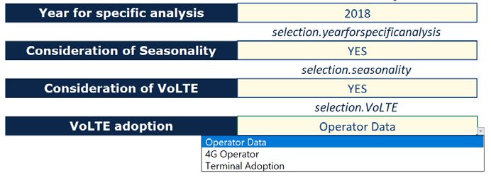
assumed to serve 4G services only. All voice VoLTE adoption
Operator Data
demand will be provided over VoLTE. Service Category Technology 2015 2016 2017 2018 2019 2020 2021 2022
Voice GSM 99,00% 96,00% 93,00% 80,40% 69,50% 58,40% 40,20% 27,20%
• Scenario 3: An operator assumed to serve Voice
Voice
UMTS
LTE
1,00%
-
4,00%
-
7,00%
-
16,60%
3,00%
25,30%
5,20%
33,00%
8,60%
48,70%
11,10%
60,80%
12,00%
all users with VoLTE-ready handsets with VoLTE adoption
VoLTE. 4G Operator
Service Category Technology 2015 2016 2017 2018 2019 2020 2021 2022
These scenarios will be included concurrently in Voice GSM - - - - - - - -
Voice UMTS - - - - - - - -
the model in order to assess their impact on the
Voice LTE - - - 100,00% 100,00% 100,00% 100,00% 100,00%
estimated voice costs.
VoLTE adoption
Terminal Adoption
Service Category Technology 2015 2016 2017 2018 2019 2020 2021 2022
Voice GSM 95,70% 93,10% 86,60% 74,90% 64,50% 51,90% 38,80% 25,60%
Voice UMTS 4,30% 6,90% 8,70% 16,70% 24,20% 31,20% 37,90% 47,00%
Voice LTE - - 4,70% 8,40% 11,30% 16,90% 23,30% 27,40%
CONFIDENTIAL 51Methodological Issue 8: Introduction of VoLTE – Methodology (2/2)
Dimensioning of VoLTE requirements will be based Overview of dimensioning for VoLTE
on the technical specifications of the standard.
First, we will calculate the required physical VoLTE traffic
PRB capacity
per call
resources to support a VoLTE call.
VoLTE standard generates traffic every 20 ms.
The traffic (bytes) generated will be dependent on PRB
the voice codec and associated headers. requirements
per call
This traffic will have to be transmitted over a Erlang B
Total PRB
number of Physical Resource Blocks (PRB).
required for
VoLTE
Applying Erlang B to the number of calls in a site VoLTE calls in
the BH
will result in the capacity required for VoLTE.
This capacity will be added to the requirements VoLTE traffic
for mobile broadband over LTE.
The model will allow to analyse different scenarios Other LTE
LTE
traffic
of VoLTE traffic evolution to understand its Dimensioning
(data, sms)
sensitivity.
CONFIDENTIAL 52Contents
4.1 Volume forecasts
4.2 Allocation of joint and common costs
4.3 Economic depreciation
4.4 Seasonality
4.5 Modelling of Single-RAN costs
4.6 VoLTE
4.7 Spectrum-related costs
4.8 Other relevant inputs
CONFIDENTIAL 53Methodological Issue 9: Spectrum license costs should be defined on a
country basis and should reflect the costs faced by MNOs - Description
Spectrum licenses are typically assigned to MNOs through 800 MHz awards in Europe
auction processes. These auctions involve a relevant 1,4
1,2
investment by MNOs which varies from country to country
EUR/MHz/pop
1,0
based on population density, number of MHz, spectrum band 0,8
auctioned, PPP, etc. 0,6
0,4
The current model considers an average annualised price of
0,2
2.5 €/inhabitant (independent of the number of MHz and the -
band), which entails some limitations: IT PL DE ES PT UK SE SK
2600 MHz (FDD) awards in Europe
• The real value of spectrum is not considered.
1,4
• Differences across markets are not reflected. 1,2
EUR/MHz/pop
1,0
• Differences in spectrum bands’ value not assessed.
0,8
0,6
0,4
Proposed approach (summary): Define actual
0,2
spectrum costs per country in terms of CapEx and OpEx
-
per MHz and band. SE UK IT SK PT ES PL DE
Source: Axon Consulting spectrum award database
CONFIDENTIAL 54Methodological Issue 10: The amount of MHz per spectrum band
should be accurately defined on a country basis - Description
We observe that, while spectrum bands for mobile services Harmonized spectrum in the EU
DE
are harmonized by the RSPG, the amount of spectrum PL
LV
available per band and country differs among SE
% of harmonized spectrum assigned to MNOs
LT
member states. SK
EE
The consideration of such divergences would entail an FI
RO
improvement in the methodology, as potential divergences IE
AT
among countries would be better recognised. UK
ES
PT
On top of that, the usage of the available spectrum per BE
EU28
underlying access technology needs to be carefully EL
IT
assessed too, as there may be limitations in terms of the HU
DK
usability of the different spectrum bands per technology. FR
NL
CZ
SI
LU
Proposed approach (summary): The real amount of CY
HR
spectrum (in MHz) and its distribution per technology BG
MT
(2G, 3G, 4G) will be defined per EU/EEA country.
- 50% 100%
Source: EC Digital Economy and Society Index 2017
CONFIDENTIAL 55Methodological Issue 11: The amount spectrum available and its split
per access technology should vary over time - Description
In the past few years, NRAs have auctioned relevant Sample spectrum awards since 2014
1.200
amounts of spectrum and operators have refarmed
MHz assigned to MNOs
1.000
technology-based historic bands. This results in a yearly
800
dependent spectrum allocation. 600
400
200
The model will consider spectrum (and its allocation to -
DE EL SI CZ FR
technologies) variable over time to better recognise the Before 2014 2014 2015 2016
realities faced by MNOs in EU/EEA.
Source: EC Digital Economy and Society Index 2014-2016
Spectrum usage by an EU/EEA MNO
200
MHz per technology
150
100
Proposed approach (summary): Introduce spectrum 50
forecasts based on operators’ expected refarming and -
2014 2015 2016 2017 2018 2019 2020 2021
upcoming spectrum auctions in EU/EEA countries.
GSM UMTS LTE
CONFIDENTIAL 56Methodological Issue 9-11: Spectrum costs and allocation trends -
Methodology (1/2)
The spectrum included in the model Illustrative example of the model’s spectrum inputs
will be representative of the COUNTRY 1
Country 1
holdings by all operators in each Technology Spectrum 2015 2016 2017 2018 2019 2020 2021 2022
GSM SPEC.900MHz 60 60 60 60 60 52 52 52
EU/EEA market. GSM SPEC.1800MHz 30 30 30 30 30 30 30 30
UMTS SPEC.900MHz - - - - - - - -
UMTS SPEC.2100MHz 30 30 60 60 90 90 90 90
For each country, we will divide the LTE SPEC.700MHz - - - - - - - -
LTE SPEC.800MHz - - - - - - - -
spectrum available in each band evenly LTE
LTE
SPEC.900MHz
SPEC.1800MHz
-
-
-
-
-
-
-
-
-
-
-
60
-
80
-
80
LTE SPEC.2100MHz - - - - - - - -
according to the market share (1/# of LTE SPEC.2600MHz - - - - - - - -
MNOs).
When dividing this spectrum, we will
COUNTRY 2
ensure that the result is consistent, Country 2
Technology Spectrum 2015 2016 2017 2018 2019 2020 2021 2022
with the standard channel/carrier size GSM
GSM
SPEC.900MHz
SPEC.1800MHz
25
-
25
-
25
-
25
-
25
-
17
-
17
-
17
-
UMTS SPEC.900MHz - - - - - 10 10 10
of access technology (modularity). UMTS SPEC.2100MHz 20 20 20 20 20 20 30 30
LTE SPEC.700MHz - - - - - - - -
LTE SPEC.800MHz - - - - - - - -
This spectrum will be used to LTE SPEC.900MHz - - - - - - - -
LTE SPEC.1800MHz - - - - - 20 20 20
determine the coverage network for LTE SPEC.2100MHz - - - - - - - -
LTE SPEC.2600MHz - - - - - - - -
each technology as well as the -
-
-
-
-
-
-
-
-
-
-
-
-
-
-
-
- - - - - - - -
available capacity to serve customers.
CONFIDENTIAL 57You can also read


