Mid-Epidemic Forecasts of COVID-19 Cases and Deaths: A Bivariate Model applied to the UK

Mid-Epidemic Forecasts of COVID-19 Cases and Deaths: A Bivariate Model
applied to the UK

Peter Congdon, School of Geography, Queen Mary University of London, Mile End Rd,
London E1 4NS, UK; p.congdon@qmul.ac.uk

Abstract Background. The evolution of the COVID-19 epidemic has been accompanied
by efforts to provide comparable international data on new cases and deaths. There is
also accumulating evidence on the epidemiological parameters underlying COVID-19.
Hence there is potential for epidemic models providing mid-term forecasts of the
epidemic trajectory using such information. The effectiveness of lockdown or lockdown
relaxation can also be assessed by modelling later epidemic stages, possibly using a
multiphase epidemic model. Methods. Commonly applied methods to analyze epidemic
trajectories or make forecasts include phenomenological growth models (e.g. the
Richards family of densities), and variants of the susceptible-infected-recovered (SIR)
compartment model. Here we focus on a practical forecasting approach, applied to
interim UK COVID data, using a bivariate Reynolds model (for cases and deaths), with
implementation based on Bayesian inference. We show the utility of informative priors in
developing and estimating the model, and compare error densities (Poisson-gamma,
Poisson-lognormal, Poisson-logStudent) for overdispersed data on new cases and
deaths. We use cross-validation to assess medium term forecasts. We also consider
the longer term post-lockdown epidemic profile to assess epidemic containment, using a
two phase model. Results. Fit to interim mid-epidemic data shows better fit to training
data and better cross validation performance for a Poisson-logStudent model.
Estimation of longer term epidemic data after lockdown relaxation, characterised by
protracted slow downturn and then upturn in cases, casts doubt on effective
containment. Conclusions. Many applications of phenomenological models have been
to complete epidemics. However, evaluation of such models based simply on their fit to
observed data may give only a partial picture, and cross-validation against actual trends
is also valuable. Similarly, it may be preferable to model incidence rather than
cumulative data, though this raises questions about suitable error densities for
modelling often erratic fluctuations. Hence there may be utility in evaluating alternative
error assumptions.

1. Introduction

Epidemic forecasts have been an essential element in policy decisions regarding the
COVID-19 epidemic, such as lockdown imposition and relaxation. Forecasting has been
assisted by well-organized efforts to provide international data on new cases and
deaths. These include daily updated comparative data provided by the European Centre
for Disease Prevention and Control (ECDC)
(https://www.ecdc.europa.eu/en/publications-data), and monitoring profiles provided by
John Hopkins University [1]. There is also a growing literature providing evidence on the
parameters of the COVID-19 infection (for example, case fatality ratios, serial intervals,
etc). Hence the potential occurs for epidemic models that are applicable to routinely

 1

collected data, that make use of accumulated evidence, and can provide forecasts for
epidemics observed at mid-stage. Policy decisions in many countries (imposition of
lockdowns, and later relaxation) have been made based on trends in observed numbers
of cases and deaths, while admitting these may be subject to measurement error - for
example, identified cases may understate total numbers infected; there are fluctuations
in daily new cases due to variation in daily testing; and there may be COVID-19
diagnostic errors.

Here we focus on a practical forecasting approach using routinely available data on new
cases and deaths (from ECDC) to estimate parameters in a bivariate version of the
Reynolds phenomenological model. Implementation is based on Bayesian inference
principles, incorporating accumulated evidence on relevant parameters via informative
priors. The operation and utility of this approach is demonstrated using data on new
cases and deaths in the United Kingdom (UK), with a focus on predictive accuracy for
20-day ahead forecasts of cases and deaths, based on mid-epidemic data. Other policy
relevant parameters such as the effective reproduction ratio and case fatality ratio are
also estimated in analysis of longer term epidemic data.

The use of a bivariate approach provides originality compared to existing research,
which, in the case of phenomenological models, is limited to analysing incidence only.
Some studies have mentioned how the mortality curve parallels the epidemic curve [2],
and we formalize these linkages under a bivariate approach. The benefits of a bivariate
approach include the ability to monitor and forecast severity measures such as the case
fatality ratio. We also consider issues in modelling daily incidence and new deaths, as
opposed to cumulative incidence and mortality. There are methodological issues in
analysing cumulative outcomes, discussed below, but also questions (not so far
considered in the literature) on how best to represent the overdispersion present in
uncumulated outcomes. The analysis below provides new evidence on the relative fit
and forecasting performance of different ways of representing Poisson overdispersion,
and shows that the usually adopted negative binomial performs less well than other
options.

The implications of the research are that effective medium term forecasts of COVID-19
incidence and mortality can be provided by the proposed methodology. Such forecasts
are useful in planning healthcare provision and assessing closeness to full capacity in
hospital bed occupancy [3, 4]. At the time of writing, daily COVID-19 hospitalisation data
were not available for the UK. However, extension of the bivariate approach to include
incidence, mortality and hospitalisations provides additional scope for forecasting of
indicators relevant to severity assessment [5, 6]. Another possible outcome in a
multivariate model is recovered cases [cf. 4], with a focus then on the ratio of predicted
recovered to predicted confirmed cases as an indicator of care need and effectiveness
of interventions. The methodology also presents a way to monitor longer term infection
numbers leading to early detection of incipient upturns in infection numbers, via
continuous monitoring and forecasting of the effective reproduction ratio.

 2

In the following sections, we review relevant literature and research gaps (section 2),
and set out the methodology (section 3). We then consider aspects of the UK case
study application (section 4), present the results (section 5), and discuss the
implications of the study's findings and methodology in the context of broader research
(section 6). Section 7 provides concluding remarks.

2. Related Research and Research Gaps
Commonly applied approaches to quantitative modelling of aggregate epidemic data
differ in the data inputs they require, their assumptions, their estimability, and in their
scope for practical application to making forecasts. Commonly applied methods include
phenomenological growth models [7], such as the Richards family of densities [8], and
variants of the susceptible-infected-recovered (SIR) compartment model [9].
Phenomenological models are parameterised in terms of epidemic trajectories and
provide estimates of crucial epidemiological parameters [10, 11], while avoiding the
complexity of more formal mechanistic models of disease transmission, which can be
difficult to estimate and provide forecasts, and may not be realistic approximations to
real epidemic dynamics [2,9,12].

As mentioned by Chowell et al [13], phenomenological models are "particularly suitable
when significant uncertainty clouds the epidemiology of an infectious disease". By
contrast, as noted in [14], compartmental transmission models may be based on
untested assumptions such as random mixing between all individuals in a given
population, may be sensitive to starting assumptions, and may provide estimates that
differ considerably between models. Such models often rely on preset parameters,
which may mean prediction uncertainty is understated. They may also be complex to
specify when an epidemic has more than one phase, whereas multiphase
phenomenological models [15] are available.

Regarding forecasts, the study by Zhao et al [16] exemplifies application of
phenomenological models to forecasts of the Zika epidemic in 2015. Autoregressive
modelling of new cases, with potential for short term forecasting, is illustrated (for foot
and mouth disease) by the first order autoregressive model of Lawson et al [17], while
(for multiple spatial units) the model of Bracher and Held [18] specifies a first order
autoregression based on the mean incidence in adjacent areas.

Regarding the COVID-19 epidemic in particular, studies with differing methodologies
have been made, some of which forecast different aspects of the COVID epidemic or
related health care need. In its impact on policy making in the UK and US, perhaps
most influential has been the Imperial College model [19]. This is based on
microsimulation with transmission through contacts between susceptible and infectious
individuals in various settings, or randomly in the community, depending on spatial
distance between contacts. A number of epidemic parameters (e.g. incubation periods
and basic reproduction numbers) are preset. Forecasts are provided for deaths and
hospital beds. Also providing forecasts across countries is the model of the Institute for
Health Metrics and Evaluation [14]. This has no underlying representation of epidemic

 3

dynamics, but is based on fitting a hierarchical parametric model for observed
cumulative death rates in different countries, and then projecting these forward.

Various types of time series forecast of the COVID-19 epidemic have also been made,
using ARIMA models [4,20,21], exponential smoothing [22], or autoregression in cases;
for example, the study by Johndron et al [23] postulates daily deaths as a lagged
function of earlier new cases. Applications of phenomenological models to COVID-19
incidence forecasts include [24] and [25].

One may identify some research gaps in the existing literature. Thus existing
applications (e.g. [24] in the case of COVID-19) have most commonly been to incidence
data, and have not considered interplay between outcomes in terms of a bivariate
model. However, examples of potentially interlinked bivariate outcomes from COVID-19,
and other epidemics, include incidence and mortality, and incidence and
hospitalizations. The paper [26] converts COVID-19 incidence, mortality and case
fatality into beta variables and applies univariate beta regression models to each
outcome. The paper [4] applies separate ARIMA models to incidence and recovered
cases. However, separate univariate regressions or time series models do not reflect
potential interlinkages between the processes that facilitate the setting of model
assumptions, or in the case of Bayesian analysis, facilitate the setting of priors on model
parameters. Regarding forecasting, wider experience of time series modelling (with non-
epidemic applications) shows the benefit of borrowing strength over outcomes [27].

Furthermore, many existing applications, such as [11, 26] in the case of COVID-19, [28]
in the case of H1N1 and Ebola, and [10] in the case of Zika, have been to cumulative
incidence. However, the drawbacks of studying cumulative incidence have been pointed
out [29, 30]. Cumulative incidence data have serially correlated measurement error,
leading to understatement of parameter uncertainty. As stated in [30], "independence of
sequential measurement errors, ... is clearly violated when observations are
accumulated through time". However, estimation using new cases or deaths
(uncumulated) puts a much greater focus on how to deal with stochastic variation in the
data. For daily data, fluctuations in new events may be considerable (including daily
"spikes"), whereas cumulative cases and deaths are usually smooth functions. There
are choices in how to model the overdispersion in new events, based on Poisson
mixtures [31], but in the epidemic literature, use of the negative binomial is standard,
and no evaluations of its relative performance are available in the literature so far.

3. Methods

3.1 Phenomenological Models
Basic phenomenological models for epidemic trajectories include the logistic, Gompertz,
and Rosenzweig, which have been the basis for a range of generalizations [7, 8].
Application of the logistic model to COVID-19 is exemplified by the studies of Batista
[32] and Shen [33]. For time , the logistic model for new cases ′ and cumulative
cases is

 4

Ct
 C ′ t  rCt 1 − K
 , 1
 Ct  K
 ,
 1e −rt− L 

where is the maximum number of cases (final epidemic size), 0 measures the
intensity of exponential growth in cases in the early epidemic phase, and is the
inflection point where new cases are highest. The Richards model [34] modifies the
logistic incidence function to
 Ct a
 C ′ t  rCt 1 − K
 , 2
with solution
 Ct  K
 1/a
 .
 1e −rt−

The parameter 0 modifies the incidence decline phase of the logistic, that is
measures the extent of deviation from the standard logistic curve. The turning point ,
when incidence peaks, is obtained when equals 1 / [35]. The peak
incidence is important for the healthcare planning, for example aligning the forecast
peak with hospital bed capacity [36].

Other commonly used models are the Gompertz model [37] with
 C ′ t  rCt logK/Ct,
while the Rosenzweig model [28] has
 Ct a
 C ′ t  rCt K
 −1 .

The incidence function represented by ′ can be used to define mean incidence in
statistical likelihoods for new cases data. Thus time series of incidence counts can often
be satisfactorily modelled as a Poisson, with means defined by ′ functions [38, 39].
Similarly the cumulative cases function can be used to define mean epidemic size
in models for cumulative case counts [28, 40].

While for smaller epidemics, a Poisson density for mean incidence may be applied, for
larger epidemics such as COVID-19, a negative binomial density is often preferred, both
because of large incidence counts, and to represent often erratic incidence fluctuations
that lead to overdispersion relative to the Poisson [30]. However, the literature does not
contain any evaluations of the negative binomial to represent overdispersion. There are
a number of other overdispersed versions of the Poisson that can be achieved by
mixing the Poisson with a suitable density (e.g. a lognormal density) [31,41], and this
may be beneficial in detecting unusual observations.

3.2 Model Specification: Poisson Overdispersion

Consider the Richards model parameters. Let and denote incidence and
cumulative incidence counts at times 1, . . . , (days in the case of COVID data
from ECDC). We condition on the first case or cases (i.e. the first observation), and take
incidence at time as a function of cumulative cases at 1, so that for a Poisson
 5

model for cases (with subscript for parameters) we have
 c t  Poisson ct  ,
  ct  r c C t−1 1 − C t−1 /K c  a c , t  2, . . . , T.
In practice, many epidemic datasets are overdispersed relative to the Poisson, and
epidemic studies generally adopt a negative binomial model instead. We can specify an
overdispersed model (including the negative binomial) by introducing multiplicative
random effects [41, eqn 2], such that the Poisson means for incidence are specified by
  ct  r c C t−1 1 − C t−1 /K c  a c  ct , 3
where the ϵct are positive random effects. For the Poisson-gamma model (equivalent
to a Negative Binomial), the ϵct are gamma distributed with mean 1, namely
  ct  Gamma c ,  c ,
where 1/ is the overdispersion parameter mentioned by [30]. Note that the
assumed parameterisation of the gamma density with random variable is
 ba
 px|a, b  Γa xa−1 e −bx .
Other options in (3) are to take as normally distributed [41]
 2
 u ct  Normal0,  uc ,
or Student t distributed [42],
 ∼ - 0, , 
where is a degrees of freedom parameter. These two options define the Poisson-
Lognormal (PLN) and Poisson-log-Student (PLS) options respectively [31]. The PLN
and PLS representations may provide a more robust alternative to the Poisson-gamma
[41, 42, 43, 44, 45], as their tails are heavier than for the gamma distribution, and have
been found to be better at accommodating outliers (such as daily "spikes" in an
epidemic application).

3.3 A Joint Model for New Cases and New Deaths
In the analysis below we apply a bivariate estimation with both new cases and deaths
modelled using the Richards specification. Thus denote and as new and
cumulative deaths at time . The joint likelihood for an overdispersed Poisson model for
both outcomes then specifies
 ct  Poisson ct ,
 d t  Poisson dt ,
  ct  r c C t−1 1 − C t−1 /K c  a c  ct , 4
  dt  r d D t−1 1 − D t−1 /K d  a d  dt , t  2, . . . , T. 5

For a Bayesian application, we need to specify prior densities, or priors for short, for the
parameters. For the epidemic size parameter , a diffuse prior confined to positive
values, such as a diffuse gamma density - for example 1, or , ,
with small - was found to lead to convergence problems. As noted in [32],"... in the
early stage, the logistic curve follows an exponential growth curve, so the estimation of

 6

 is practically impossible". This difficulty persists when an epidemic is past its peak
but early in a downturn.

However, Batista [32] mentions a relationship (for the logistic model) between
successive cumulative case counts that may assist in providing a prior for .
Specifically for three points spaced time units apart, one may obtain the relationship
for a point estimator of , namely
 C t−m C t−2m C t−m −2C t−2m C t C t−m C t 
 K ec  .
 C 2t−m −C t C t−2m 
One may use this point estimator to define a prior mean for in the Richards model
(which is a generalisation of the logistic). Specifically, one may take a lognormal density
prior for , with as mean, and a suitable variance, such that the prior is still
relatively diffuse. For example, suppose is 250,000, and the variance in the
lognormal is set at 1. Then the 97.5 percentile for the lognormal prior is 1.77 million.

In the bivariate specification (for new cases and new deaths jointly), we seek to share
prior information between outcomes. One option for the prior on (the final death
total) is as a function of , namely
 Φ ,
where Φ is a form of case fatality ratio (CFR). An informative prior for Φ could be based
on the COVID experience in similar countries, or on experience of epidemics of similar
diseases. Considering the first option, and an appropriate prior for analysing UK data,
an informative prior for Φ could be provided by the case fatality ratio across the
European Union (the UK being no longer an EU member). International information on
case fatality is provided at https://ourworldindata.org/mortality-risk-covid#the-current-
case-fatality-rate-of-covid-19.

Alternatively one may link and using both the point estimator and a case
fatality ratio, namely Φ . Then a lognormal density prior can be taken for ,
with Φ as the mean, and a suitable variance such that the
prior is still relatively diffuse.

Another possible prior to link ultimate cases and deaths would involve a time series in
time-specific case fatality ratios , such as an autoregression ∼ , ,
with estimated from cumulative data on deaths and cases. Some analyses of
epidemics show that the CFR early in an epidemic may underestimate later values [46],
in which case the prior on Φ may be constrained to exceed the final based on
observed data. With regard to COVID-19 this pattern may not necessarily apply, with
the US (for example) showing a decline in CFRs at later epidemic stages. There is also
evidence that the mortality to infection ratio (a more precise measure than the CFR) has
fallen [47].To allow for such a scenario, the prior for Φ could be centred at the last
observed , rather than constrained to exceed it.

Joint priors on other parameters could be considered, for example, bivariate normal
priors on the logs of and , or on the logs of and . In the empirical
 7

analysis below we focus on priors linking the final epidemic and death total parameters,
 and , as these are an important influence on forecasts.

3.4 Medium Term Forecasts
Many applications of phenomenological models are to historic data on epidemics, where
the epidemic has run to its full extent. Here we consider applications to incomplete
epidemics (e.g. epidemics observed to their mid point or early in the downturn), and to
forecasts using such data. Forecasts at an intermediate point within the observation
span are of interest in themselves for policy purposes. However, they can also be used
in comparative model evaluation by using cross-validation, with only some data used for
estimating the model, and some held out for validation.

Thus suppose the training sample is formed by observations up to time , while
the subsequent observations at times 1, . . . , (where are
used as a validation sample. Predictions , and , for new cases and
deaths at time 1 are based on observed cumulative counts and . As
usual in Bayesian inference, predictions are obtained as replicate data sampled from
the posterior predictive densities | | , , and | 
 | , where , are data on new cases and deaths, and are
parameters in the joint model of section 3.3 [48].

Predicted cumulative counts at time 1 are then obtained as , ,
 , and , , . Predicted new cases and deaths at 
2 , namely , and , are then sampled from the appropriate
phenomenological model form, based on , and , . Cumulated cases
and deaths at 2 are then obtained by adding predicted new cases and deaths for
 2 to , and , . This process is continued until time .

Fit can be assessed by whether credible intervals for predictions in the cross-validation
period include actual incidence and new deaths. Also relevant are probabilities of over
or under-prediction. For example, consider predicted new cases , , for the
validation period 1, . . . , , and for MCMC samples 1, . . . , , and let
average new predicted cases during the validation period (the average over days) at
iteration be denoted , , : . We want to compare average predicted new
cases with average observed new cases, : , during the validation period.
Probabilities of overprediction can be obtained from binary indicators
 O c
 s  Ic new,s,T1:TF  c T1:TF , s  1, . . . , S,
where 1 if condition is true, and 0 otherwise. Thus at each iteration
we compare average new cases (modelled) during the validation period with actual
average new cases.

Probabilities of overprediction for new cases, , are estimated as ∑s=1,…,S / .
Probabilities of underprediction can be obtained as 1 . A satisfactory prediction

 8

would have 0.05 0.95, with over 0.95 indicating a high probability of
overprediction, while under 0.05 indicates a high probability of underprediction.
Underprediction means under-forecasting of future cases, and may lead to incorrect
inferences regarding epidemic control, as it implies a lessening in incidence earlier than
actually occurred.

3.5 Longer Term Epidemic Monitoring, Effective Reproduction Ratios and Case Fatality
Ratios
Strategic decisions regarding containment of the COVID-19 epidemic, in the UK and
other countries, have depended on trends in new infections and deaths, but also on the
effective reproduction rate. Thus in the UK the choice on whether or not to relax the
initial COVID lockdown restrictions was based on five criteria, with two being numeric:
first, "a sustained and consistent fall in daily death rates", and second that the "rate of
infection is decreasing to manageable levels", meaning that the effective reproduction
ratio is demonstrably below 1. The reproduction rate may also become especially
relevant at later epidemic stages (post-lockdown), after a downturn from the initial peak
and after lockdown measures have been relaxed. Here the concern is to prevent a
resurgence of infection, indicated by an upturn in .

In the case of a protracted downturn, but with new cases still occurring, the concern is
especially that there may be a substantial resurgence in cases, and possibly also
deaths, at some point. This scenario is colloquially known as a "second wave", and in
most European countries there have been pronounced second waves in the COVID-19
epidemic during 2020, albeit at different times. Such a resurgence indicates use of a
multiphase model [15], with a second phenomenological model applied to data after a
latent switch-point between epidemic regimes. Note that at the time of writing (August
2020) a fully developed second wave had not yet happened in the UK, though the signs
were of an upturn in , as the analysis below confirms.

In planning for hospital care, longer term trends in disease severity may be relevant. For
example, an upturn in cases may reflect more cases among younger people at lower
mortality risk. Hence trends in, and forecasts of, the case fatality rate are an important
aspect of strategic management. In a bivariate model of cases and deaths, as here, we
can trace the modelled CFR through time, where the modelled CFR at day is given by
the ratio of predicted total deaths to predicted total cases , / , . In a natural
extension of the bivariate model to include hospitalisations, trends in, and forecasts of,
hospitalisation rates (ratios of hospitalised cases to total cases) can also be made.

Assume there is some evidence from new cases data of an upturn in cases, even
before a second wave epidemic is fully established. Consider a model for new cases
only. Then a two phase model to reflect the upturn would involve two phenomenological
models, before and after a latent switch-point, with each model having distinct
parameters. Denote the single switch-point in new cases as , such that for a two-
 9

phase Richards model
 ct  Poisson ct 
  ct  It  c r c1 C t−1 1 − C t−1 /K c1  a c1   It ≥ c rc2 C t−1 1 − C t−1 /K c2  a c2 
where 1 when condition is true, and 0 otherwise. Parameters, such as
( , ) are differentiated by outcome and by wave. The parameter can be assigned
a uniform prior (on a positive interval) or a positive valued prior, such as an exponential
density. If there is a second wave upturn in deaths also, then a bivariate model can be
used, with switch points assumed later for deaths than cases, due to possible
delays in mortality upturns following incidence upturns. A three phase model for cases
would have two switch-points, with mean
  ct  It   c1 rc1 C t−1 1 − C t−1 /K c1  a c1  
I c2  t ≥ c1 r c2 C t−1 1 − C t−1 /K c2  a c2   It ≥ c2 r c3 C t−1 1 − C t−1 /K c3  a c3 .

An estimator of the effective reproduction rate at time is based on predictions from
this phenomenological model, and from an estimate of the serial interval density. The
serial interval is the time between symptom onset in an infected subject and symptom
onset in the infectee. The serial interval density can discretized in the form of weights
 , applied to serial interval lengths (in days) up to a maximum . These can be used
to estimate effective reproduction ratios within a phenomenological model to analyse
new cases; see the papers [38], [49] and [50]. Thus can be estimated as
 J
 R t  c new,t / ∑  jcnew,t−j,
 j0
where , are predicted new case data from the phenomenological model. By virtue
of the MCMC sampling strategy used below, we can readily obtain 95% credible
intervals for , and the probability that 1, which is important for assessing
epidemic containment strategy.

4. Model Application
We consider the application of the above methods to UK data on new cases and deaths
from 1st February 2020 (when the first two cases of COVID-19 in the UK were reported
according to ECDC). Observations are assigned dates as in the ECDC data, with times
 in days from 1st February 2020. Figures 1a and 1b show daily trends in these
outcomes up to 8th August 2020, with erratic fluctuations apparent in both outcomes.
However, there is a broad downward trend in both outcomes from days 70 to 80, though
with a more protracted decline as opposed to the steep initial upturn. Figures 2a and 2b
show the relatively smooth evolution of cumulative cases and deaths.

4.1 Medium Term Forecasts
For medium term forecasts, we focus on the Richards bivariate model (section 3.3) and
compare three alternative error assumptions as discussed in section 3.2: Poisson-
Gamma (PG), Poisson-lognormal (PLN) and Poisson-log-Student (PLS). The Student
density is represented by a scale mixture of normals [51, 52]. Thus for new cases,

 10

instead of directly taking
 u ct  t0,  2uc ,  c ,
where is the degrees of freedom parameter, and where , we take
 ct  Gamma 2c , 2c ,
  2uc
 u ct  N0,  ct
 ,
The indicators have average 1, but are significantly lower than 1 for more outlying
observations, such as daily spikes in cases.

Cross-validation estimations are made at points . Thus we consider twenty day
ahead forecasts at three different stages of the UK COVID-19 epidemic. For the first
cross validation, estimations are based on training data up to day 80 with 
20 (i.e. the cross validation period consists of days 81 to 100 ). Cross validation
estimations with 20 are also made for 100, and for 120 , with forecast
accuracy based on comparing forecasts with hold out data for days 1, . . . , .

4.2 Model Assumptions
For prior densities on the unknowns in the medium term forecasts, exponential priors
with mean 1 are assumed on , , and . For the precisions 1/ and
1/ in the PLN and PLS options, and for the parameters and in the
Poisson-gamma model, a gamma prior 1,0.001 is assumed. For the PLS
option, we take 4 as a preset option. The degrees of freedom can be difficult
to estimate for relatively small datasets, and the option of the preset value 4 is a
robust option [53, 54]. For the maximum cases (epidemic size) parameter , we
assume as lognormal prior, centred at (with m=5 in ) and with variance 1,
as discussed in section 3.2.

For the maximum deaths parameter , we assume Φ where the prior for
Φ is a beta density with mean defined by the EU-wide case fatality . The beta has
total prior count set at 5, 5 . Thus the prior on Φ is Φ ~ , 1
 . For example, on 20-04-2020 (at day 80 ), the EU wide case fatality rate
was 0.101, and the prior is set at Φ ∼ 0.505,4.495 . This illustrates the use of
relevant external information, rather than diffuse priors.

4.3 Model Fit and Estimation
Fit to the observed training data is assessed using the Watanabe--Akaike information
criterion (WAIC) [55]. This is a fit measure which takes account of fit but also penalizes
model complexity. Cross-validation fit (fit out of the observed sample) is assessed by
the probabilities of forecasting overprediction, and , and by predictive
coverage: whether the credible intervals for predicted cases and deaths (averages over
each validation period) include the observed averages. Estimation uses the BUGS
program [56], with posterior estimates based on the second halves of two chain runs of
100,000 iterations, and convergence assessed using Brooks-Gelman-Rubin criteria
[57].

 11

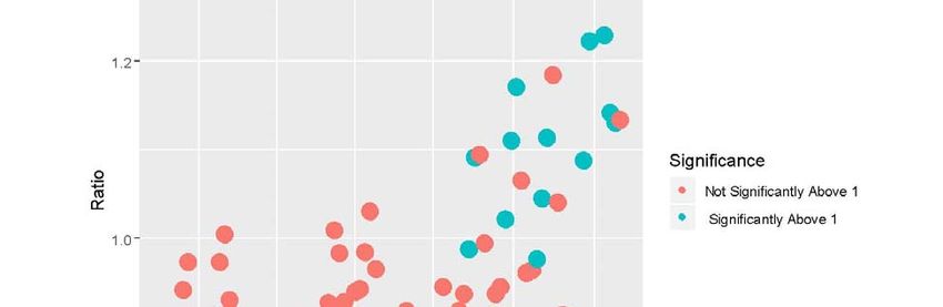
4.2 Modelling Later Epidemic Stages
To provide a longer term perspective on epidemic containment, we apply the best
performing model from analysis of the first wave to the full set of observations as at 8th
August 2020 (T=190), when the first epidemic peak had passed. So this application is to
a situation where the epidemic first wave has passed, but there are still non-negligible
numbers of new cases, and a potential for possible upturns and further waves.

New cases and deaths (as 7 day moving averages) had reached maxima of 4850 and
950 respectively when the UK epidemic peaked in April 2020. As a result of lockdown
measures imposed in late March, daily new cases averaged just over 500 daily by July.
However, lockdown relaxations from July were accompanied by the risk of resurgence.
In that regard, an upturn was apparent with new cases in late July and early August
averaging over 800 daily (see Figure 3), though deaths continued to fall, averaging
around 50 per day in early August.

To model the full time series, and since there was no upturn in deaths apparent in early
August 2020, we focus on new cases only. To reflect the evidence of an upturn in
cases, a two phase model is applied. For this model, the shift parameter is assigned
an exponential prior density with mean 150. Priors on the parameters of the second
phase Richards model are as before for the exponential ascent and logistic modifier
parameters. For (the forecast total cases under wave 2), we assume 
with assigned an exponential prior with mean 1. Of policy interest here is epidemic
containment, as summarised by the effective reproduction ratio: specifically the question
of policy relevance is whether this ratio consistently below 1, and whether its 95%
credible interval also entirely below 1. If the ratio is not below 1, this suggests a
significant upturn.

To provide estimates of the effective reproduction ratio, we use accumulated evidence
on COVID serial intervals from five studies [58,59,60,61,62]. A gamma density on the
serial interval (SI) is assumed, and information on mean and standard deviation of the
SI, or on quantiles of SI, is converted to gamma density parameters; for use of SI
quantiles in this regard, see [63]. Large samples (of a million) from each the five
densities are taken, and parameters of the pooled gamma density are estimated from
the pooled sample of five million; the pooled gamma density has shape 1.38 and rate
0.36. This density is then converted to a discretized form (with 16 bins) to provide an
informative prior on the SI to the model of White and Pagano [64], which updates the
prior serial interval density using new case data for the UK. The paper [65] recommends
that the initial, approximately exponential, epidemic phase be used in estimation, and
we use UK new case data up to time 24-04-2020, when UK new cases peaked [see 55,
page 3]. The updated mean serial interval is estimated as 3.5 days with standard
deviation 3.1. The discretized serial interval is estimated as in [64], with in section 3.5
set at 16.

5. Results

 12

5.1 Table 1 compares parameter estimates from the observed (training) data under the
three error assumptions for the three cross-validation analyses at M=80, M=100 and
M=120 (i.e. nine scenarios). It should be noted that predictions of cases and deaths
should be based not on the posterior mean or median parameter values in Table 1, but
on sampled posterior predictive replicate data at each iteration. These are based on
sampling new data from the Poisson means (4) and (5), and from the Richards model
parameter profile at each particular iteration. The predicted values of cases and deaths
are very close to actual values: for example, for the PLS model at M=120, the average
absolute deviation (over 2, . . ,120) between actual new cases and predicted new
cases is under 1. Table 2 compares the WAIC fits to the observed data under the nine
options, while criteria regarding 20 day ahead forecasts are shown in Table 3.

5.2 Mid Term Forecasts.
Table 1 shows broad consistency between the three distributional options in terms of
estimated final epidemic size and eventual death total . The posterior density of
these parameters may be skewed, with posterior mean exceeding median. For the PLN
and PLS options the estimate of increases as does. This reflects the
protracted nature of the UK downturn in cases after the peak in the first wave. Posterior
mean estimates of the turning points and vary slightly and tend to be higher for
 100 and 120, but for both outcomes and all values are between 72 and
86. Turning point estimates for new cases are also mostly higher under the PLS
option.

Table 2 shows that the PLS option has better fit, with lower WAIC values. Hence its
estimates of epidemic size and turning points are preferred, and provide a better
description of the slow decline in cases from their peak. Table 3 shows generally better
cross-validation performance for the PLS option. As discussed above, satisfactory
prediction would have 0.05 0.95, and 0.05 0.95, with or 
over 0.95 indicating overprediction, and with or under 0.05 indicating
underprediction. Both PG and PLN options show underprediction for higher values of
 , and in policy terms, may be misleading in suggesting a faster decline in cases and
deaths than actually occurred. By contrast for 100 and 120 , the 95%
interval for predicted average cases under the PLS model comfortably includes the
actual average new cases.

5.3 Longer Term Scenario
Estimates of policy relevant parameters also come from the longer term scenario when
the log-Student Richards model is applied to UK COVID new case data up to day T=190
(8th August, 2020). The shift point in the two phase model is estimated as 179.1 with
95% interval from 179.0 to 179.3.

Figure 4 plots out the posterior mean estimated effective reproductive ratios (5 day
moving averages), distinguishing those estimates significantly above 1. The estimates
hover around 1 throughout June and the first half of July, but in late July/early August
tend to exceed 1. The impression from this is that success in fully effective containment
 13

is then in doubt. The estimates of the reproduction ratio, and their path through June
and July, are similar to those for the UK available at
https://epiforecasts.io/covid/posts/national/united-kingdom/#national-summary and
based on the methods in [66].

To illustrate the potential for longer term forecasts of severity indicators we also use
observed data up to day 150 to make forecasts 40 days ahead through to day 190. This
analysis uses the PLS model option. Figure 5 shows the resulting forecast of the case
fatality ratio, with 95% intervals, with a slight downward trend apparent. The interval for
 190 includes the observed value of 0.151.

6. Discussion
The existing epidemic modelling literature has recognized the need for overdispersed
distributions to deal with erratic incidence counts [67, 68, 30]. Thus [68] shows that use
of a negative binomial distribution is more appropriate than the Poisson for describing
emerging infections with overdispersed case distributions due to superspreading
events. However, so far as the authors are aware there has been no evaluation of the
negative binomial as compared to other methods of representing overdispersion in
epidemic counts. Hence one contribution of this paper rests on a comparison of the
negative binomial (Poisson-gamma mixture) against alternative Poisson mixture models
[31]. For example, the Poisson log-Normal distribution is a longer tailed alternative to
the negative binomial distribution, and may better fit overdispersed count data [69,70].
The analysis here suggests such alternatives may usefully be considered as
alternatives to the negative binomial, and may both improve fit to actual observations
and provide more accurate forecast performance.

Tackling overdispersion is one issue present in modelling count data associated with
epidemics. Another is the outcome focus: the choice is between incidence alone (the
usual approach), or on taking account of both incidence and related outcomes. We have
developed here a bivariate approach to jointly modelling epidemic outcomes, using
priors that link parameters between outcomes. For example, here the eventual death
total is linked (via the Bayesian prior specification) to the eventual epidemic size
 . This approach has been used here to study the interrelationships between incidence
and mortality, but can be readily extended to more outcomes, such as incidence,
mortality, and hospitalisations. Forecasts from such joint outcome models enable
forecasts of epidemic severity (e.g. case fatality rates, case-hospitalization ratios,
deaths-hospitalizations ratios as well as effective reproduction ratios) that assist in
pandemic severity assessment. Severity assessment, and the development of summary
indicators of epidemic severity, is being recognized as an important aspect of epidemic
monitoring and modelling [71, 72].

The present paper also considers the gain in applying phenomenological models to later
stages of incomplete epidemics, especially (in the case of COVID-19) after lockdown
relaxations, where there may be a protracted period of non-zero incidence, or further
more pronounced waves of infection. The above analysis has therefore applied the

 14

Poisson-log Student to late epidemic data for the UK (up to early August 2020), when
there was some evidence of an incidence upturn, but not yet a full blown second wave.
The focus of this analysis was on the effective reproduction rate and the case fatality
ratio, both indicators of epidemic severity. As mentioned in [73], "the COVID-19
pandemic has shown that the effective reproduction rate of the virus is a crucial
determinant not only of public health, but also of public policy". There are a number of
ways of estimating this quantity, including novel approaches such as using Google
mobility data [74]. Here an analysis using estimates of based on a two-phase
Richards model suggest a upturn in transmission in the UK by late July/early August
2020.

Hence the added value of the study is provided by the following: (a) proposing a
multivariate framework readily applied for assessing severity, (b) in providing an
approach for assessing alternative methods for representing overdispersion; and (c) in
providing a methodology for assessing long terms trends and making longer term
forecasts (e.g. of case fatality and the effective reproduction rate) in a multi-wave
situation.

7. Conclusion

Many applications of phenomenological models have been to complete epidemics.
However, evaluation of such models based simply on their fit to observed data may give
only a partial picture. Also relevant to epidemic model assessment, particularly for policy
application, is the accuracy of medium term forecasts for incomplete epidemics.
Arguably, evaluation in this case is better done using a cross-validation approach,
where only some of the observed data are used to estimate parameters, and a hold out
sample can then assess the accuracy of forecasts. The analysis here of UK epidemic
data in the first half of 2020 has shown that fit to training data and the cross validation fit
are consistent in their choice of preferred model option.

The contribution of the present paper is to illustrate a bivariate approach to two
epidemic outcomes, and how prior information (under a Bayesian approach) can be
applied to interlink the parameters governing each outcome. The benefits of a bivariate
(and potentially multivariate) approach include the ability to forecast severity measures
such as the case fatality ratio, and the borrowing of strength over outcomes in making
forecasts [27]. A further contribution is that a focus on incidence and new deaths rather
than cumulative outcomes has brought into sharper focus the question of adequately
representing Poisson overdispersion. The latter is caused by often erratic fluctuations in
the observed series, apparent in UK COVID data on new cases and deaths. The
analysis has provided new evidence on the relative fit and forecasting performance of
different ways of representing Poisson overdispersion in epidemic count data, and
potential gains through using heavier tail alternatives to the negative binomial. We have
also considered Bayesian analysis of longer term epidemic trends, where multiple
waves may exist, and illustrated monitoring of case fatality and epidemic reproduction.

 15

The implications of the research (e.g. in planning healthcare provision) are that effective
medium term forecasts of COVID-19 incidence and mortality can be provided by the
proposed methodology. Extension of the bivariate approach (e.g. to include incidence,
mortality and hospitalisations) provides scope for forecasting other indicators relevant to
severity assessment. The methodology also presents a way to monitor longer term
infection numbers leading to early detection of incipient upturns in infection numbers,
via continuous monitoring and forecasting of the effective reproduction ratio. Assessing
whether the latter is confined to values below 1 is important for strategic epidemic
containment.

The present study has some possible limitations. Comparative analysis of alternative
ways of representing overdispersion has been limited here to UK data, and to the first
wave COVID-19 epidemic, and will require validation with other epidemic time series,
both for COVID-19 and other infectious diseases. A caveat, though not a limitation per
se, is that with regard to Bayesian estimation, relatively informative priors may be
needed to guarantee stable estimation and ensure convergence. For example, diffuse
gamma priors on the eventual epidemic size parameter caused convergence problems
in the analysis reported here.

Regarding future research, as just pointed out, the methodology for comparing
overdispersion approaches should be assessed with other epidemic datasets. Other
Poisson mixtures may be considered such as the Poisson log skew-normal [75], or
Poisson mixtures with other densities [76,77]. Other types of analysis regarding
forecasting potential can also be envisaged, such as forecast combinations, for
instance, forecasts based on combining the logistic, Richards and Gompertz curves [78,
79]. It would also be useful, especially in planning hospital care capacity, to apply a
bivariate approach to COVID-19 incidence and hospitalisations, or a trivariate approach
to incidence, mortality and hospitalisations. A trivariate approach will provide model
estimates and forecasts of indicators central to severity assessment.

Competing Interests: The authors declare no competing interests.

References
[1] Dong E, Du H, Gardner L. An interactive web-based dashboard to track COVID-19 in
real time. The Lancet Infectious Diseases. 2020 Feb 19.
[2] Ma J. Estimating epidemic exponential growth rate and basic reproduction number.
Infectious Disease Modelling. 2020, 5:129-41.
[3] Cavallo J, Donoho D, Forman H. Hospital capacity and operations in the coronavirus
disease 2019 (COVID-19) pandemic---planning for the nth patient. In JAMA Health
Forum 2020 Mar 2 (Vol. 1, No. 3, pp. e200345-e200345). American Medical
Association.
[4] Maleki M, Mahmoudi M, Wraith D, Pho K. Time series modelling to forecast the
confirmed and recovered cases of COVID-19. Travel Medicine and Infectious Disease.
2020, 13:101742.

 16

[5] Centre for Disease Control and Prevention (CDC). Pandemic Severity Assessment
Framework (PSAF). https://www.cdc.gov/flu/pandemic-resources/national-
strategy/severity-assessment-framework.html
[6] Reed C, Biggerstaff M, Finelli L, Koonin LM, Beauvais D, Uzicanin A, Plummer A,
Bresee J, Redd SC, Jernigan D. Novel framework for assessing epidemiologic effects of
influenza epidemics and pandemics. Emerging Infectious Diseases. 2013, 19(1):85
[7] Bürger R, Chowell G, Lara-Diaz L. Comparative analysis of phenomenological
growth models applied to epidemic outbreaks. Mathematical Biosciences and
Engineering: 16(5):4250-73, 2019
[8] Tjørve E, Tjørve KM. A unified approach to the Richards-model family for use in
growth analyses: why we need only two model forms. Journal of theoretical biology.
267(3):417-25, 2010
[9] Roda, W, Varughese, M, Han, D, Li, M. Why is it difficult to accurately predict the
COVID-19 epidemic? Infectious Disease Modelling, 5, 271-281, 2020.
[10] Zhao S, Musa S, Fu H, He D, Qin J. Simple framework for real-time forecast in a
data-limited situation: the Zika virus (ZIKV) outbreaks in Brazil from 2015 to 2016 as an
example. Parasites and Vectors. 12(1):344, 2019.
[11] Macêdo A, Brum A, Duarte-Filho G, Almeida F, Ospina R, Vasconcelos G. A
comparative analysis between a SIRD compartmental model and the Richards growth
model. https://www.medrxiv.org/content/10.1101/2020.08.04.20168120v1.full.pdf
[12] Loberg S, Lehman C. Applying the unified models of ecology to forecast epidemics,
with application to COVID-19. MedRxiv.https://doi.org/10.1101/2020.04.07.20056754,
2020.
[13] Chowell G, Sattenspiel L, Bansal S, Viboud C. Mathematical models to characterize
early epidemic growth: A review. Physics of Life Reviews. 2016, 18:66-97.
[14] Institute for Health Metrics and Evaluation (IHME) Forecasting covid-19 impact on
hospital bed-days, ICU-days, ventilator days and deaths by us state in the next 4
months. MedRxiv,https://doi.org/10.1101/2020.03.27.20043752. 2020.
[15] Hsieh Y, Cheng Y. Real-time forecast of multiphase outbreak. Emerging Infectious
Diseases. 2006, 12(1):122
[16] Zhao S, Musa S, Fu H, He D, Qin J. Simple framework for real-time forecast in a
data-limited situation: the Zika virus (ZIKV) outbreaks in Brazil from 2015 to 2016 as an
example. Parasites and Vectors. 12(1):344, 2019.
[17] Lawson A, Onicescu G, Ellerbe C. Foot and mouth disease revisited: re-analysis
using Bayesian spatial susceptible-infectious-removed models. Spatial and Spatio-
temporal Epidemiology, 2(3):185-94, 2011.
[18] Bracher J, Held L. Endemic-epidemic models with discrete-time serial interval
distributions for infectious disease prediction. arXiv preprint, arXiv:1901.03090, 2019
[19] Imperial College COVID-19 Response Team. Impact of non-pharmaceutical
interventions (NPIs) to reduce covid-19 mortality and healthcare demand.
https://www.imperial.ac.uk/mrc-global-infectious-disease-analysis/covid-19/report-9-
impact-of-npis-on-covid-19/, 2020.
[20] Chintalapudi N, Battineni G, Amenta F. COVID-19 disease outbreak forecasting of
registered and recovered cases after sixty day lockdown in Italy: A data driven model
approach. Journal of Microbiology, Immunology and Infection, 53, 396-403, 2020.

 17

[21] Bayyurt L, Bayyurt B. Forecasting of COVID-19 Cases and Deaths Using ARIMA
Models. MedRxiv. https://doi.org/10.1101/2020.04.17.20069237, 2020.
[22] Petropoulos F, Makridakis S. Forecasting the novel coronavirus COVID-19. PloS
One. 15(3):e0231236, 2020.
[23] Johndrow J, Lum K, Gargiulo M, Ball P. Estimating the number of SARS-CoV-2
infections and the impact of social distancing in the United States. ArXiv,
https://arxiv.org/abs/2004.02605, 2020.
[24] Roosa K, Lee Y, Luo R, Kirpich A, Rothenberg R, Hyman J, Yan P, Chowell G.
Short-term forecasts of the COVID-19 epidemic in Guangdong and Zhejiang, China.
Journal of Clinical Medicine. 9(2):596, 2020
[25] Pancrazi R. Estimating and forecasting COVID-19 evolution in the UK and its
regions.
https://warwick.ac.uk/fac/soc/economics/research/centres/cage/publications/bn20.2020.
pdf, 2020.
[26] De Oliveira R, Achcar J, Nunes A. Modeling the incidence and death rates of
COVID-19 pandemic in different regions of the world. Epidemiologic Methods. 2020
https://doi.org/10.1515/em-2020-0017.
[27] Du Preez J, Witt S. Univariate versus multivariate time series forecasting: an
application to international tourism demand. International Journal of Forecasting. 2003,
19(3):435-51.
[28] Liu, W., Tang, S, Xiao, Y. Model selection and evaluation based on emerging
infectious disease data sets including A/H1N1 and Ebola. Computational and
Mathematical Methods in Medicine, 2015.
[29] Grad Y, Miller J, Lipsitch M. Cholera modeling: challenges to quantitative analysis
and predicting the impact of interventions. Epidemiology, 2012, 23(4):523.
[30] King A, Domenech de Cellès M, Magpantay F, Rohani P. Avoidable errors in the
modelling of outbreaks of emerging pathogens, with special reference to Ebola.
Proceedings of the Royal Society B: Biological Sciences. 282(1806):20150347, 2015
[31] Karlis D, Xekalaki E. Mixed Poisson distributions. International Statistical Review.
73(1):35-58, 2005.
[32] Batista M. Estimation of the final size of the coronavirus epidemic by the logistic
model. MedRxiv. https://www.medrxiv.org/content/10.1101/2020.03.11.20024901v2,
2020
[33] Shen, C. Logistic growth modelling of COVID-19 proliferation in China and its
international implications. International Journal of Infectious Diseases, 96,582-589,
2020.
[34] Hsieh Y. Richards model: a simple procedure for real-time prediction of outbreak
severity. In "Modeling and Dynamics of Infectious Diseases", World Scientific, eds Zhien
Ma, Yicang Zhou, Jianhong Wu, pp. 216-236, 2009
[35] Wang X, Wu J, Yang Y. Richards model revisited: Validation by and application to
infection dynamics. Journal of Theoretical Biology. 313:12-19, 2012
[36] Linton O. When will the coronavirus pandemic peak?. LSE Business Review.
https://blogs.lse.ac.uk/businessreview/2020/04/07/when-will-the-coronavirus-pandemic-
peak/, 2020
[37] Jia L, Li K, Jiang, Y, Guo, X. Prediction and analysis of Coronavirus Disease 2019.

 18

ArXiv preprint arXiv:2003.05447, 2020.
[38] Chowell G, Hincapie-Palacio D, Ospina J, Pell B, Tariq A, Dahal S, Moghadas S,
Smirnova A, Simonsen L, Viboud C. Using Phenomenological Models to Characterize
Transmissibility and Forecast Patterns and Final Burden of Zika Epidemics. PLOS
Currents Outbreaks. doi:
10.1371/currents.outbreaks.f14b2217c902f453d9320a43a35b9583, 2016
[39] Viboud C, Simonsen L, Chowell G. A generalized-growth model to characterize the
early ascending phase of infectious disease outbreaks. Epidemics. 15:27-37, 2016.
[40] Bauckhage C, The Math of Epidemic Outbreaks and Spread (Part 3) Least Squares
Fitting of Gompertz Growth Models.
https://www.researchgate.net/profile/Christian_Bauckhage/publication/
[41] Zhou M, Li L, Dunson D, Carin L. Lognormal and gamma mixed negative binomial
regression. In Proceedings of the International Conference on Machine Learning, Vol.
2012, 1343-1350, 2012
[42] Gaver, D, O'Muircheartaigh, I. Robust empirical Bayes analyses of event rates.
Technometrics, 29(1), pp.1-15, 1987.
[43] Sohn, S. A comparative study of four estimators for analyzing the random event
rate of the Poisson process. Journal of Statistical Computation and Simulation, 49(1-2),
1-10, 1994
[44] Trinh G, Rungie C, Wright M, Driesener C, Dawes J. Predicting future purchases
with the Poisson log-normal model. Marketing Letters, 25(2):219-34, 2014
[45] Connolly, S, Dornelas, M., Bellwood, D, Hughes, T. Testing species abundance
models: a new bootstrap approach applied to Indo-Pacific coral reefs. Ecology, 90,
3138--3149,2009.
[46] Böttcher L, Xia M, Chou T. Why estimating population-based case fatality rates
during epidemics may be misleading. medRxiv 2020.03.26.20044693; doi:
https://doi.org/10.1101/2020.03.26.20044693
[47] Vaughan A. Getting less deadly? New Scientist, Volume 247, Issue 3297, page 7.
[48] Gelman, A. A Bayesian formulation of exploratory data analysis and goodness-of-fit
testing. International Statistical Review, 71(2),369-382, 2003.
[49] Cori A, Ferguson N, Fraser C. A new framework and software to estimate time-
varying reproduction numbers during epidemics. Am J Epidemiol, 178(9): 1505--12,
2013
[50] Nishiura H, Chowell G. The effective reproduction number as a prelude to statistical
estimation of time-dependent epidemic trends. In: Mathematical and Statistical
Estimation Approaches in Epidemiology 2009 (pp. 103-121). Springer, Dordrecht.
[51] Peel, D, McLachlan, G. Robust mixture modelling using the t distribution. Statistics
and Computing, 10(4), 339-348, 2000
[52] Moravveji B, Khodadadi Z, Maleki M. A Bayesian analysis of two-piece distributions
based on the scale mixtures of normal family. Iranian Journal of Science and
Technology, Transactions A: Science. 2019, 43(3):991-1001.
[53] Gaver D, Jacobs P, O'Muircheartaigh I. Regression analysis of hierarchical
poisson-like event rate data: superpopulation model effect on predictions.
Communications in Statistics-Theory and Methods. 19(10):3779-97, 1990
[54] Gelman A, Carlin J, Stern H, Dunson D, Vehtari A, Rubin D. Bayesian Data

 19

Analysis, 3rd Edition (Chapman & Hall/CRC), 2013.
[55] Watanabe, S. A Widely Applicable Bayesian Information Criterion. Journal of
Machine Learning Research. 14: 867--897, 2013.
[56] Lunn, D, Thomas, A., Best, N, Spiegelhalter, D (2000) WinBUGS --- a Bayesian
modelling framework: concepts, structure, and extensibility. Statistics and Computing,
10:325--337
[57] Brooks, S, Gelman, A. (1998) General methods for monitoring convergence of
iterative simulations. Journal of Computational and Graphical Statistics, 7, 434-455.
[58] Bi Q, Wu Y, Mei S, Ye C, Zou X, Zhang Z, Liu X, Wei L, Truelove S, Zhang T, Gao
W. Epidemiology and transmission of COVID-19 in 391 cases and 1286 of their close
contacts in Shenzhen, China: a retrospective cohort study. The Lancet Infectious
Diseases. https://www.thelancet.com/pdfs/journals/laninf/PIIS1473-3099(20)30287-5,
2020
[59] Cereda D, Tirani M, Rovida F, Demicheli V, Ajelli M, Poletti P, Trentini F, Guzzetta
G, Marziano V, Barone A, Magoni M. The early phase of the COVID-19 outbreak in
Lombardy, Italy. arXiv preprint arXiv:2003.09320. 2020.
[60] Chan Y, Flasche S, Lam T, Leung M, Wong M, Lam H, Chuang S. Transmission
dynamics, serial interval and epidemiology of COVID-19 diseases in Hong Kong under
different control measures. Wellcome Open Research. 11;5(91):91, 2020
[61] Nishiura H, Linton N, Akhmetzhanov A. Serial interval of novel coronavirus (COVID-
19) infections. International Journal of Infectious Diseases. 93, 284-286, 2020.
[62] Du Z, Xu X, Wu Y, Wang L, Cowling B, Meyers L. Serial interval of COVID-19
among publicly reported confirmed cases. Emerging Infectious Diseases. 26(6):1341-
1343, 2020
[63] Belisle, P. 2012. Computing gamma distribution parameters by
gamma.parms.from.quantiles().
http://www.medicine.mcgill.ca/epidemiology/Joseph/PBelisle/GammaParmsFromQuantil
es.html.
[64] White L, Pagano M. A likelihood-based method for real-time estimation of the serial
interval and reproductive number of an epidemic. Statistics in medicine. 27(16):2999-
3016, 2008
[65] Obadia T, Haneef R, Boëlle PY. The R0 package: a toolbox to estimate
reproduction numbers for epidemic outbreaks. BMC Medical Informatics and Decision
Making. 2012, 12(1):1-9.
[66] Abbott S, Hellewell J, Thompson R, Sherratt K, Gibbs H, Bosse N, Munday J,
Meakin S, Doughty E, Chun J, Chan Y. Estimating the time-varying reproduction
number of SARS-CoV-2 using national and subnational case counts. Wellcome Open
Research. 2020 Jun 1;5(112):112.
[67] An Q, Wu J, Fan X, Pan L, Sun W. Using a negative binomial regression model for
early warning at the start of a hand foot mouth disease epidemic in Dalian, Liaoning
province, China. PloS one. 2016, 11(6):e0157815.
[68] Tuite A, Fisman D. The IDEA model: A single equation approach to the Ebola
forecasting challenge. Epidemics. 2018, 22:71-77.
[69] Izsák R. Maximum likelihood fitting of the Poisson lognormal distribution. Environ
Ecol Stat. 2008;15(2):143--156.

 20