Spatio-temporal assessment of annual water balance models for upper Ganga Basin - HESS
←
→
Page content transcription
If your browser does not render page correctly, please read the page content below
Hydrol. Earth Syst. Sci., 22, 5357–5371, 2018
https://doi.org/10.5194/hess-22-5357-2018
© Author(s) 2018. This work is distributed under
the Creative Commons Attribution 4.0 License.

Spatio-temporal assessment of annual water balance models
for upper Ganga Basin
Anoop Kumar Shukla1 , Shray Pathak1 , Lalit Pal1 , Chandra Shekhar Prasad Ojha1 , Ana Mijic2 , and Rahul Dev Garg1
1 Department   of Civil Engineering, Indian Institute of Technology Roorkee, Uttarakhand, India
2 Department   of Civil and Environmental Engineering, Imperial College London, London, UK

Correspondence: Shray Pathak (shraypathak@gmail.com)

Received: 30 August 2017 – Discussion started: 6 September 2017
Revised: 30 January 2018 – Accepted: 5 April 2018 – Published: 18 October 2018

Abstract. The upper Ganga Basin in Uttarakhand, India, has        timation of water yield further facilitates in the identifica-
high hydropower potential and plays an important role in the      tion of hotspots for storm-water harvesting in order to fulfill
development of the state economy. Thus, an accurate knowl-        fresh-water demand in the region (Pathak et al., 2017). The
edge of annual water yield is of paramount importance to          hydrological ES are dependent on different factors, such as
this region. This paper deals with use of contemporary wa-        watershed characteristics (e.g., topography, land use and land
ter yield estimation models such as the distributed Integrated    cover – LULC, soil type and climatic condition. To incorpo-
Valuation of Ecosystem Services and Tradeoffs (InVEST)            rate these parameters into assessment and decision-making,
model and the Lumped Zhang model and their validation to          there has been a proliferation of ecosystem-modeling tools
identify the most suited one for water yield estimation in the    and methods. Models for ES evaluation often focus on using
upper Ganga Basin. In previous studies utilizing these mod-       globally available data, accepting large number of spatially
els, water yield was estimated by considering a single value      explicit inputs producing spatially explicit output, and limit-
of some important model parameters for the entire basin,          ing the model structure to key biophysical processes involved
which in fact show distributed variation at a finer (pixel)       in land use change (Guswa et al., 2014). The precise estima-
scale. Therefore, in this study, pixel-level computations are     tion of ES using these models is a complicated task owing
performed to assess and ascertain the need for incorporat-        to spatial variability and dependence of ES on various to-
ing the spatial variation of such parameters in model appli-      pographical and climatic factors. Further, the validation and
cations. To validate the findings, the observed sub-basin dis-    uncertainty assessments in model outputs have proven to be
charge data are analyzed with the computed water yield for        key obstacles to the application of ES models. In the litera-
4 decades, i.e., 1980, 1990, 2001 and 2015. The results ob-       ture, studies focusing on comparison of different ES models
tained are in good agreement with the water yield obtained at     have projected some light over the model output validation
the pixel scale.                                                  issues; however, a lack of studies highlighting the validation
                                                                  of these models for Indian river basins still exists. The ben-
                                                                  efits that can be derived from ES should be analyzed and
                                                                  quantified in a spatially explicit manner (Sánchez-Canales et
1   Introduction                                                  al., 2012). The uncertainties involved in the determination
                                                                  of spatial and temporal distribution of the climatic variables,
An accurate assessment of key ecosystem services (ES) such        especially precipitation, constitute a major obstacle to the un-
as water yield has gained focus in recent years in ES mod-        derstanding of hydrological behavior at the catchment scales
eling, as fresh-water availability in a region is essential       (Milly and Dunne, 2002).
for agriculture, industry, human consumption, hydropower,            The Integrated Valuation of ES and Tradeoffs (InVEST)
etc. (Redhead et al., 2016). Hydrological ecosystem services      model, developed by Natural Capital Project (Tallis et al.,
generally include drinking water supply, power production,        2010), is a tool that provides a framework for planners and
industrial use, irrigation and many more. The accurate es-

Published by Copernicus Publications on behalf of the European Geosciences Union.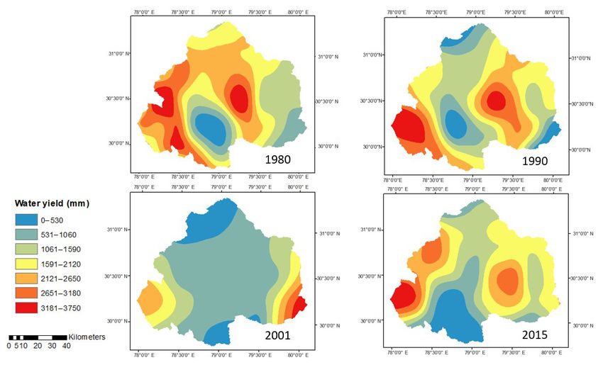
5358            A. K. Shukla et al.: Spatio-temporal assessment of annual water balance models for upper Ganga Basin

decision makers to assess trade-offs among ES and enables         pothesis. Several attempts have later been made to obtain
their comparison in various climate and land use change sce-      an analytical solution of the Budyko hypothesis (Schreiber,
narios. The model includes a biophysical component, which         1904; Ol’Dekop, 1911; Turc, 1954; Mezentsev, 1955; Pike,
facilitates the provision of fresh water or water yield from      1964; Fu, 1981; Choudhury, 1999; Zhang et al., 2001, 2004;
different parts of the landscape, and a valuation component,      Porporato et al., 2004; Yang et al., 2008; Donohue et al.,
representing the benefits of water provisioning to people. The    2012; Wang and Tang, 2014; G. Zhou et al., 2015; S. Zhou
model works on simplified Budyko theory, which has a long         et al., 2015). Among these studies, solutions provided by
history and still continues to receive attention in the hydro-    Fu (1981) called Fu’s equation, gained significant attention
logical literature (Budyko and Ronov, 1979; Zhang et al.,         as the work represented the effect of catchment properties on
2001; Zhang et al., 2004; Ojha et al., 2008; Zhou et al., 2012;   water balance components by incorporating an addition pa-
Donohue et al., 2012; Xu et al., 2013; Wang and Tang, 2014).      rameter “w”. Fu’s equation can provide a full picture of the
The InVEST model applies a one-parameter formulation of           evaporation mechanism at the annual timescale. Therefore,
the Budyko theory in a semi-distributed manner (Zhang et          Fu’s equation can be used through a top-down analysis for
al., 2004). The model is capable of quantifying the water         providing insight into the dynamic interactions among cli-
yield of a catchment under the influence of change in differ-     mate, soils, vegetation, and their controls on the annual water
ent drivers, viz. climate variables and catchment characteris-    balance at the regional scale (Yang et al., 2007).
tics (e.g., land use change). Various studies have been carried      Considering the lack of studies on analysis and validation
out in the past demonstrating the application of the InVEST       of ES on the Indian subcontinent, especially for Himalayan
model to different river basins around the world. Sánchez-        catchments, and to assess the applicability of various water-
Canales et al. (2012) carried out a sensitivity analysis of       balance models to Himalayan catchments, the present work
three parameters, i.e., z (seasonal precipitation coefficient),   attempts to compute and analyze water yield in the upper
precipitation (annual) and ET0 (annual reference evapotran-       Ganga Basin using a semi-distributed InVEST model and a
spiration), and using the InVEST model for a Mediterranean        Lumped Zhang model. The work primarily considers, in de-
basin, they found precipitation to be the most sensitive pa-      tail, the spatial variation of InVEST model parameters and
rameter for the study region. Later, Terrado et al. (2014) ap-    uses different strategies to compute water yield. Accordingly,
plied the InVEST model for the heavily inhabited defined as       water yield is estimated for 4 years, i.e., 1980, 1990, 2001
Llobregat river basin. The model is applied for both extreme      and 2015 and the most appropriate strategy is identified. The
wet and dry conditions, and the role of climatic parameters       parameters that are adopted as lumped at the basin scale in
is emphasized. Hoyer and Chang (2014) applied this model          previous studies are estimated at the pixel scale in order to
in the Tualatin and Yamhill basins of northwestern Oregon         avoid the dependence of the model parameters on size of
under a series of urbanization and climate-change scenarios.      the catchment. In addition, pixel-level estimations of water
The results show that the climatic parameters have more sen-      yield are expected to be more accurate than output obtained
sitivity than other inputs for a water yield model. Hamel and     using the conventional approach with basin-lumped output.
Guswa (2015) applied the same water yield model for the           The term “finer scale” in the paper represents the incorpora-
Cape Fear catchment, North Carolina, and concluded that the       tion of spatial variations through the pixel-level estimation of
precipitation is the most influencing parameter. Goyal and        parameters involved in InVEST model, which are otherwise
Khan (2017) employed the InVEST water yield model for the         taken as lumped. The work also compares the outcomes of
hilly catchment by considering two catchments, i.e., the Sut-     spatially distributed water yield models and the convention-
lej River catchment and Tungabhadra River catchment. The          ally used Lumped Zhang model.
climate parameters, i.e., precipitation and ET0 , are observed
to be the most influencing parameters for water yield in both
the river basins. With the aforementioned studies, certain fac-   2     Background theory
tors exist that limit the application of InVEST model such as
                                                                  2.1     Water yield models
the absence or inadequate comparison with observed data,
the calibration of the model without prior identification of      In this section, two water yield models, i.e., the InVEST
sensitive parameters and a lack of validation of the predictive   water yield model, which is a distributed model, and the
capabilities in the context of land use and land cover change     Lumped Zhang model, are described.
(Bai et al., 2012; Nelson et al., 2010; Su and Fu, 2013; Ter-
rado et al., 2014).                                               2.1.1    InVEST model
   The InVEST model operates on the principle of the
Budyko theory (Budyko, 1958, 1974). Based on works of             The InVEST water yield model (Tallis et al., 2010) is de-
Schreiber (1904) and Ol’Dekop (1911), Budyko proposed             signed to provide information regarding the changes in the
formulations explaining the relationship between precipita-       ecosystem that are likely to alter the flow. It is based on the
tion and potential evapotranspiration (PET) in order to cou-      Budyko theory, which is an empirical function that yields
ple water and energy balances, defined as the Budyko hy-          the ratio of actual to potential evapotranspiration (PET)

Hydrol. Earth Syst. Sci., 22, 5357–5371, 2018                                   www.hydrol-earth-syst-sci.net/22/5357/2018/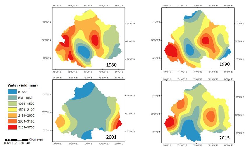
A. K. Shukla et al.: Spatio-temporal assessment of annual water balance models for upper Ganga Basin                        5359

(Budyko, 1979). To describe the degree to which long-term           adjusted by Kc (x) for each pixel over the map of land use and
catchment water balance deviates from the theoretical limits,       land cover. w(x) is an empirical parameter, and the expres-
a number of scholars have proposed one-parameter functions          sion given by Donohue et al. (2012) for the InVEST model
that can replicate the Budyko curve (Fu, 1981; Choudhury,           has been applied to define w(x), which is expressed as fol-
1999; Zhang et al., 2004; Wang and Tang, 2014). To observe          lows:
and represent pixel-level changes to the landscape, InVEST
                                                                                 AWC(x)
model incorporates, explicitly, the spatial variability in pre-     w(x) = z ×          + 1.25.                                (4)
cipitation, PET, soil depth and vegetation. The model oper-                       P (x)
ates at the grid scale and acquires the inputs in the raster for-   Thus, the minimum value of the parameter w(x) is 1.25, cor-
mat into a GIS environment such as ArcGIS.                          responding to bare soil where the root depth is zero (Dono-
   The InVEST water yield model is based on an empirical            hue et al., 2012). The Donohue model was originally de-
function known as the Budyko curve (Budyko, 1974). An-              veloped for Australia, however, the online documentation
nual water yield, Y (x), is determined at each pixel of a land-     on InVEST model states its application globally. The pa-
scape as follows;                                                   rameter z is known as the seasonality factor whose value

                AET(x)
                                                                   varies from 1 to 30. It represents the nature of local precip-
Y (x) = 1 −               × P (x),                            (1)   itation and other hydrogeological parameters. The parame-
                 P (x)
                                                                    ter AWC(x) depicts volumetric plant available water content
where AET(x) is the actual annual evapotranspiration per            expressed in depth (mm), which can be expressed by follow-
pixel x and P (x) is the annual precipitation per pixel x. Ac-      ing formula for each pixel x:
tual evapotranspiration (AET) is essentially determined by
climatic factors (precipitation, temperature, etc.) and is me-      AWC(x) = Min.(Restricting layer depth, root depth) × PAWC. (5)
diated by catchment characteristics (vegetation cover, soil
                                                                    The root-restricting layer depth is defined as the depth of
characteristics, topography, etc.). On the other hand, poten-
                                                                    the soil up to which the soil can allow the penetration of
tial evapotranspiration (PET) represents the evaporating po-
                                                                    the roots, and root depth is defined as the depth where
tential of the climate system at a specific location and time
                                                                    95 % of the root biomass occurs. Plant available water con-
of year without the consideration of catchment characteris-
                                                                    tent (PAWC) is generally taken as the difference between
tics and soil properties (Allen et al., 1998). Several attempts
                                                                    the field capacity and the wilting point. It depends upon the
have been made in the past to establish a relationship be-
                                                                    soil properties and can be computed by the Soil-Plant-Air-
tween AET and PET, among which the solution provided
                                                                    Water (SPAW) software. In the study, PAWC is calculated
by Fu (1981) has been adopted worldwide. Fu (1981) pro-
                                                                    using the method described by McKenzie et al. (2003). The
vided an analytical solution to the Budyko hypothesis and
                                                                    modified Hargreaves method and Hargreaves method were
related AET with PET by incorporating a dimensionless pa-
                                                                    employed for computing reference evapotranspiration for the
rameter “w”, which denotes the effect of catchment charac-
                                                                    study area at pixel scale.
teristics.
                                                                    The modified Hargreaves method is expressed as
   The InVEST model uses the expression of the Budyko
curve proposed by Fu (1981) and Zhang et al. (2004). The            ET0 = 0.0013 × 0.408 × RA × Tavg + 17.0

ratio of mean annual PET to annual precipitation, known as
index of dryness, is expressed as                                       × (TD − 0.0123 × P )0.76 ,                             (6)

                                            1                     where ET0 is reference evapotranspiration, Tavg is the av-
AET(x)      PET(x)      PET(x)                w
       = 1+        − 1+                            ,         (2)    erage daily temperature (◦ C) defined as the average of
 P (x)       P (x)       P (x)                                      mean daily maximum and mean daily minimum temper-
where PET(x) is the annual potential evapotranspiration per         ature, TD (◦ C) is the temperature range computed as the
pixel x (mm), and w(x) is a non-physical parameter that in-         difference between mean daily maximum and mean daily
fluences the natural soil properties. The PET(x) is calculated      minimum temperature, and RA is extraterrestrial radiation
using the following expression;                                     (MJ m−2 day−1 ).
                                                                    According to the Hargreaves method,
PET(x) = Kc (x) × ET0 (x),                                   (3)
                                                                    ET0 = 0.0023 × 0.408 × RA × Tavg + 17.8 × TD0.5 , (7)


where ET0 (x) is the annual reference evapotranspiration per
pixel x, which is computed based on evapotranspiration from         where terms involved in the equation means same as those in
alfalfa grass grown at that location using Eq. (6). Kc (x) is the   the modified Hargreaves method.
vegetation evapotranspiration coefficient that is influenced           For computing the extraterrestrial radiation (RA), the fol-
by the change in characteristics of land use and land cover         lowing equation is used;
at every pixel (Allen et al., 1998). The values of ET0 (x) are

www.hydrol-earth-syst-sci.net/22/5357/2018/                                      Hydrol. Earth Syst. Sci., 22, 5357–5371, 2018
5360             A. K. Shukla et al.: Spatio-temporal assessment of annual water balance models for upper Ganga Basin

         24(60)
RA =            × Gsc × dr × [ws sin(ϕ) sin(δ)
           π
      + cos(ϕ) cos(δ) sin (ws )] ,                         (8)

where RA is extraterrestrial radiation (MJ m−2 day−1 ), dr is
the inverse Earth–Sun relative distance, Gsc is the solar
constant equal to 0.0820 MJ m−2 min−1 , ws is sunset hour
angle (rad), δ is the solar declination (rad) and ϕ is lati-
tude (rad).

Determination of the parameter “w”

The dimensionless parameter w depends upon the local cli-
matic variables such as the hydrological characteristics of
the area, its rainfall intensity and topography. In the InVEST
water yield model (Tallis et al., 2010), parameter w can be
computed in three different ways. The first method is sug-
gested by Donohue et al. (2012), in which parameter w is
computed using Eq. (4) and where sensitivity parameter z is
adopted as one fifth of the number of rain events per year.
                                                                  Figure 1. Graphical representation of the study area, the upper
The second method is suggested by Xu et al. (2013), which         Ganga Basin.
compares w with latitude, the NDVI (normalized difference
vegetation index), area, etc. The third method experiments
with various selections of w (one value of w for the entire       About 60 % of the basin is utilized for agricultural practices,
study region) until there is a good match between observed        and 20 % of the basin is in the forest area, especially in the
and computed water yield. Unfortunately, this method is not       upper mountainous region. Nearly 2 % of the basin is perma-
suited for a pixel-based analysis, as the number of pixels will   nently covered with snow in the mountain peaks. The most
be extremely large, making the method computationally in-         predominant soil groups found in the region are sand, clay,
tensive.                                                          loam and their compositions. In the upper Ganga Basin, the
                                                                  average annual rainfall varies from 550 to 2500 mm (Bharati
2.1.2    Lumped Zhang model                                       et al., 2011), where a major fraction of total annual rainfall is
                                                                  received during monsoon months (June–September). The ge-
In this model, the mean value of different parameters is used     ographical location and other information of the upper Ganga
as an input to compute the average value of the water yield       Basin are represented in Fig. 1.
for the whole watershed. The average actual evapotranspira-
tion, potential evapotranspiration, w, precipitation, etc., are   3.2     Data
described by Zhang et al. (2004).
                                                                  3.2.1    Precipitation and temperature

3     Study area and data                                         The daily time series of precipitation and temperature for the
                                                                  study area are acquired from India Meteorological Depart-
3.1     Study area                                                ment (IMD) at a grid size of 0.25◦ and 1◦ , respectively. The
                                                                  upper Ganga Basin comes within the dataset latitude, which
The Ganga river in India is ranked amongst the world’s top        ranges from 29.5◦ N to 31.5◦ N, and its longitude, ranging
20 rivers in regards to the water discharge. The Ganga river      from 77.75 to 80.25◦ E . The daily time series of precipita-
is segregated into three zones, viz. the upper Ganga Basin,       tion was aggregated to obtain the annual time series at each
middle Ganga Basin and lower Ganga Basin. The area cho-           grid point. Various analyses in the study are carried out for 4
sen for the present study, i.e., the upper Ganga Basin, is sit-   years, i.e., 1980, 1990, 2001 and 2015.
uated in the northern part of India within the geographical
coordinates 29◦ 480 –31◦ 240 N and 77◦ 490 –80◦ 220 E, covering   3.2.2    Soil map
an area of 22 292.1 km2 and reaching up to Haridwar. The
altitude of the study area varies from 275 m in the plains to     Spatial maps of soil were collected from the National Bu-
7512 m in the Himalayan terrains. A region of approximately       reau of Soil Survey and Land Use Planning (NBSSLUP) at
433 km2 of the basin is located under glacier landscape, and      1 : 250 000. Digital maps of soil available at a resolution of
288 km2 of the region is located under a fluvial landscape.       1200 m × 1200 m were resampled to the resolution of land

Hydrol. Earth Syst. Sci., 22, 5357–5371, 2018                                    www.hydrol-earth-syst-sci.net/22/5357/2018/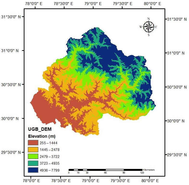
A. K. Shukla et al.: Spatio-temporal assessment of annual water balance models for upper Ganga Basin                          5361

use data, i.e., 30 m × 30 m, using “resample” tool in ArcGIS            In strategy B, the entire basin is considered for comput-
in order to maintain the scale homogeneity. The attribute ta-        ing the parameter w for large basins, using Eq. (9), which
ble of the raster layer contains fields like soil depth, soil tex-   is given by Xu et al. (2013). In strategy C, the parameter w
ture, carbon content percentage, drainage, slope, erosion, soil      is computed for entire basin using Eq. (10), which is given
temperature and mineralogy. The relevant features, i.e., soil        by Xu et al. (2013). In strategy D, parameter w is computed
depth and soil texture are converted into the raster image for       at each pixel in order to incorporate the spatial distribution
the upper Ganga Basin.                                               of the hydrologic variables involved in the computations. In
                                                                     Strategy E, parameter z is computed according to the num-
3.2.3   Map of land use and land cover                               ber of rain events in a year; subsequently, Eq. (4) is used to
                                                                     compute the parameter w.
Satellite images were acquired from different sensors of                For all the strategies, the extraterrestrial radiation (RA)
Landsat, viz. Landsat 3/4 Multispectral Scanner and The-             parameter is computed for each month using Eq. (8), and a
matic Mapper (MSS/TM), Landsat 4 Thematic Mapper                     raster layer is generated. Precipitation data are obtained from
(TM), Landsat 7 Enhanced Thematic Mapper (ETM) and                   Indian Meteorological Department (IMD) at a grid size of
Landsat 8 Operational Land Imager (OLI) sensors for the              0.25◦ for the study area. It has been interpreted and con-
years 1980, 1990, 2001 and 2015, respectively. The im-               verted to the raster format by using the inverse distance
ages are available at different resolutions and in several           weighted (IDW) interpolation technique in the ArcGIS envi-
wavelength bands, from which green (G), red (R) and near-            ronment for obtaining the values for all pixels at a resolution
infrared (NIR) band images are combined to create a false            equal to the resolution of the Landsat satellite images. The
color composite (FCC) for the study area in ERDAS Imag-              temperature dataset is obtained from the IMD at a grid size
ine. FCCs are then classified using supervised classification        of 1◦ × 1◦ for the study area and has also been converted to
in ERDAS in six different classes, i.e., forest, water, agri-        a raster format by using the IDW interpolation technique for
cultural, wasteland, snow and glacier, and built-up land. The        obtaining the values for all pixels. Subsequently, the mean
classification of the area is based on their similar response        monthly value of average temperature (Tavg ) and the differ-
under different bands. Each class is then recognized with the        ence between the mean daily maximum and mean daily min-
help of ground-truth and high-resolution satellite images.           imum (TD) are obtained. The climate datasets used in the
                                                                     present study are of the finest resolution available so far for
4    Methodology                                                     the study region. Gridded datasets of temperature and pre-
                                                                     cipitation used in the present study have been developed us-
In the present work, five different strategies are employed          ing quality-controlled stations and well-proven interpolation
to compute water yield. For the ease of presentation, these          techniques. Further details about the datasets of precipitation
strategies are referred to as A–E. In strategy A, an average         and temperature are given in Srivastava et al. (2009) and Pai
value of precipitation, temperature, extraterrestrial radiation      et al. (2014), respectively.
and parameter w is used for the entire basin. This strategy             The modified Hargreaves method is applied for obtain-
is essentially based on Lumped Zhang model. Strategies B–            ing the value of reference evapotranspiration at each pixel
E are designated, corresponding to a particular variation of         for each month (Droogers et al., 2002). To compute poten-
the InVEST model where water yield is computed using dif-            tial evapotranspiration, the yearly values obtained for the
ferent approach for estimating parameter w. For computing            reference evapotranspiration are multiplied by the vegeta-
parameter w, relationships for large basins and for the global       tion evapotranspiration coefficient (Kc ), which depends on
model from Xu et al. (2013) are given by Eqs. (9) and (10),          the LULC characteristics, as expressed in Eq. (3). The value
respectively.                                                        of Kc is taken from Allen et al. (1998), as shown in Table 1.
For large basins,                                                    In this study, Kc is taken in the same was for all 4 years, as
                                                                     shown in Table 1, and is used to obtain potential evapotran-
w = 0.69387 − 0.01042 × lat + 2.81063 × NDVI                         spiration, which is subsequently used to obtain annual water
    + 0.146186 × CTI.                                         (9)    yield at each pixel of the study area.

For the global model,
                                                                     5     Results
w = 3.50412 − 0.09311 × slp − 0.03288 × lat + 1.12312
    × NDVI − 0.00205 × long − 0.00026 × elev,                (10)    5.1    Reference evapotranspiration, ET0 (x)

where, “slp” is the slope gradient, “lat” is the absolute lati-      Reference Evapotranspiration (ET0 ) is computed for the up-
tude of basin center, “CTI” is the compound topographic in-          per Ganga Basin using a high-resolution monthly climate
dex, “NDVI” is the normalized difference vegetation index,           dataset. The modified Hargreaves method is applied for ob-
“lat” is latitude, “long” is longitude and “elev” is elevation.      taining the values of reference evapotranspiration at each

www.hydrol-earth-syst-sci.net/22/5357/2018/                                          Hydrol. Earth Syst. Sci., 22, 5357–5371, 2018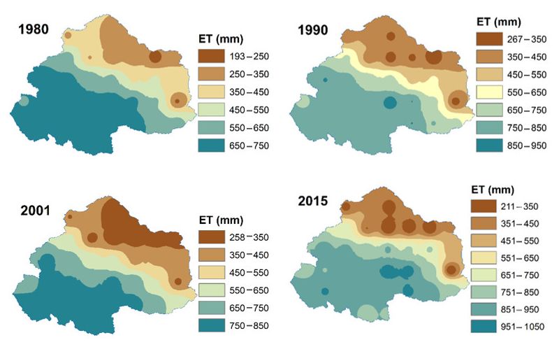
5362             A. K. Shukla et al.: Spatio-temporal assessment of annual water balance models for upper Ganga Basin

Table 1. Value of Kc corresponding to the classes of land use and land cover.

                        S. no.   Land use and        Percentage     Percentage     Percentage   Percentage    Kc
                                 land cover               cover          cover          cover        cover
                                                         (1980)         (1990)         (2001)       (2015)
                        1        Forest                    17.84         16.32         15.78         15.19      1
                        2        Water                     21.87         21.27         19.47         17.65      1
                        3        Wastelands                 51.1         52.36         54.18         55.46    0.2
                        4        Built-up area              2.07          2.14          2.27          2.49    0.4
                        5        Agricultural               3.67          4.04          3.76          4.22   0.75
                        6        Snow and glacier           3.45          3.87          4.54          4.99      2

Figure 2. Reference evapotranspiration (mm) of the upper Ganga Basin for the years 1980, 1990, 2001 and 2015.

pixel for each month (Droogers and Allen, 2002). ET0 is a               tion coefficient are taken from Table 1. Thus, the potential
function of RA, precipitation, Tavg and TD, which are com-              evapotranspiration is computed for upper Ganga Basin for
puted pixel-wise for each month of the years 1980, 1990,                the years 1980, 1990, 2001 and 2015, as represented in Fig. 3.
2001 and 2015. Some of the months, i.e., July, July and Au-
gust 1990; June, July and August 2001; and June, July and               5.3     Water yield, Y (x)
August 2015, showed negative values of reference evapotran-
spiration from applying the modified Hargreaves method. For             As described in the methodology, five different strategies,
these months, Hargreaves method is applied for obtaining the            viz. A–E, are used to estimate water yield for the upper
positive values. Subsequently, all mean monthly values are              Ganga Basin.
added up to get the mean annual values of evapotranspiration
                                                                        Strategy A: water yield computed using the Lumped
for the years 1980, 1990, 2001 and 2015, as represented in
                                                                        Zhang model
Fig. 2.
                                                                        Here, the basin average values of all the input parameters are
5.2    Potential evapotranspiration, PET(x)                             considered, and water yield is computed for the upper Ganga
                                                                        Basin for the years 1980, 1990, 2001 and 2015, which are
The annual values obtained for the ET0 are multiplied by the            obtained as 658.52, 925.68, 603.71 and 1194.25 mm, respec-
vegetation evapotranspiration coefficient (Kc ), which varies           tively.
with the characteristics of land use and land cover, as ex-
pressed in Eq. (3). The value of the Kc is taken from Allen
et al. (1998). The values of the vegetation evapotranspira-

Hydrol. Earth Syst. Sci., 22, 5357–5371, 2018                                          www.hydrol-earth-syst-sci.net/22/5357/2018/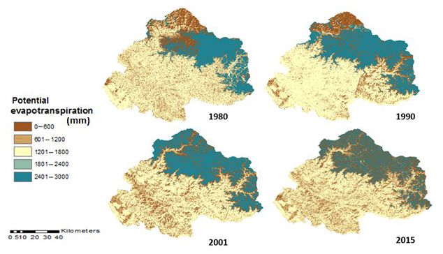
A. K. Shukla et al.: Spatio-temporal assessment of annual water balance models for upper Ganga Basin 5363
Figure 3. Potential evapotranspiration (mm) of the upper Ganga Basin for the years 1980, 1990, 2001 and 2015.
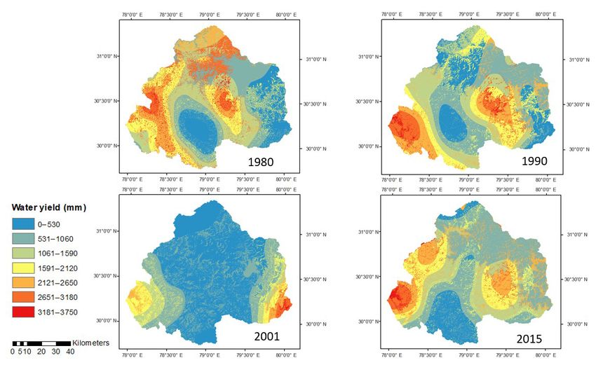
Strategy B: water yield obtained by taking the single Strategy D: water yield obtained using the pixel-level
weighted mean value of parameter “w” from Xu et estimation of parameter “w” from Xu et al. (2013)
al. (2013) for large basins
In this strategy, the values of parameter w are estimated at
In this strategy, water yield is computed by considering a the pixel level. The water yield computed for the years 1980,
single value of the parameter w for the whole basin using 1990, 2001 and 2015 for upper Ganga Basin is shown in
Eq. (9). The weighted mean value for parameter w for the Fig. 6. The mean values of water yield as computed us-
years 1980, 1990, 2001 and 2015 are obtained as 1.507, ing strategy D for the years 1980, 1990, 2001 and 2015
1.541, 1.403 and 1.507, respectively. The spatial distribution are 1240.02, 1549.44, 1149.89 and 1754.62 mm, respec-
of the water yield for the upper Ganga Basin computed using tively.
strategy B is represented in Fig. 4. The mean values of water
yield as obtained using this method for the years 1980, 1990, Strategy E: water yield obtained using the pixel-level
2001 and 2015 are 755.65, 959.48, 742.39 and 1131.42 mm, estimation of parameter “w” from Donohue et al. (2012)
respectively.
Equation (4) represents the parameter w as a function of pa-
Strategy C: water yield obtained by taking a single rameter “z”, AWC and precipitation. The parameter w in the
weighted mean value of parameter “w” from Xu et equation used in strategy E has been proposed by Donohue et
al. (2013) for the global model al. (2012), which is also cited in online documentation of In-
VEST model; however, the final equation used for estimating
In this strategy, water yield is computed by considering a water yield is obtained from the InVEST model. Considering
single value of parameter w for the entire upper Ganga this fact, Donohue et al. (2012) has been cited in strategy E.
Basin using Eq. (10). The weighted mean value of param- The water yield as computed using strategy E for the up-
eter w for the years 1980, 1990, 2001 and 2015 are obtained per Ganga Basin for different years is shown in Fig. 7. The
as −0.967, −0.955, −1.010 and −0.968, respectively. The mean values of water yield for the years 1980, 1990, 2001
spatial distribution of the water yield for the upper Ganga and 2015 are 1241.09, 1552.38, 1153.95 and 1753.53 mm,
Basin as computed using strategy C is shown in Fig. 5. The respectively.
mean values of water yield for the years 1980, 1990, 2001
and 2015 are 1239.92, 1549.46, 1149.93 and 1754.59 mm,
respectively.
www.hydrol-earth-syst-sci.net/22/5357/2018/ Hydrol. Earth Syst. Sci., 22, 5357–5371, 2018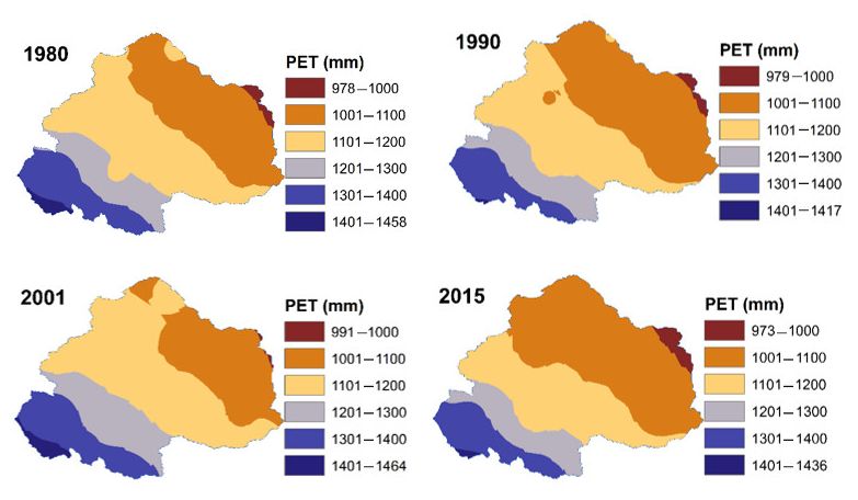
5364              A. K. Shukla et al.: Spatio-temporal assessment of annual water balance models for upper Ganga Basin

Table 2. Comparison of model-estimated PET and AET with a global dataset from different sources.

            Parameter    Year     Source 1    Source 2     Strategy A                       InVEST model
            (mm)                 (GLDAS)       (CRU)       (Lumped       Strategy B   Strategy C    Strategy D      Strategy E
                                                            Zhang            (Large      (Global     (Xu et al.     (Donohue
                                                            model)           model)       model)         2013)    et al., 2012)
            AET          1980     555.0355                   696.84         486.07        679.52        679.68         680.01
                         1990      646.168                   815.02          592.3        735.23        735.27         736.25
                         2001      588.084                   680.76         408.86        548.28        548.39         550.38
                         2015     716.8316                   900.11         625.41        743.48        743.52         744.34
            PET          1980                 1175.964      1376.64        1382.12       1382.12       1382.12        1382.12
                         1990                 1156.497      1456.16        1461.86       1461.86       1461.86        1461.86
                         2001                 1184.847      1457.08        1462.96       1462.96       1462.96        1462.96
                         2015                 1156.686      1544.20        1550.42       1550.42       1550.42        1550.42

Figure 4. Water yield obtained by taking the single weighted mean value of parameter w from Xu et al. (2013) for large basins.

5.4    Validation of ET and water yield estimates                       from the Climate Research Unit’s (CRU’s) PET datasets
                                                                        (CRU TS v. 4.01) available at resolution of 0.5◦ . From the
                                                                        comparison, both AET (GLDAS) and PET (CRU TS) values
For validation of model outputs, the basin’s average annual             are found to be in fair agreement with the globally estimated
values of PET and AET estimated using various strategies                values (Table 2). Spatial maps of global datasets of AET and
are compared with the corresponding basin average values                PET are shown in Figs. 8 and 9, respectively.
obtained from available global datasets (Table 2). Model-                  The validation of water yield obtained from various strate-
simulated AET values are obtained from the Global Land                  gies is performed at the Rishikesh gauging site of the upper
Data Assimilation System (GLDAS) ET dataset from Noah                   Ganga Basin (Fig. 10). The discharge data of the basin are
model outputs. Basin average values of PET are obtained

Hydrol. Earth Syst. Sci., 22, 5357–5371, 2018                                         www.hydrol-earth-syst-sci.net/22/5357/2018/
A. K. Shukla et al.: Spatio-temporal assessment of annual water balance models for upper Ganga Basin                                 5365

Table 3. Observed vs. computed water yield for various proposed strategies for Rishikesh sub-basin.

     Strategies                                                                              1980       1990       2001      2015
     Observed discharge (mm)                                                              1831.31     2422.43   2187.22    2835.81
     Observed discharge (mm) (after reducing approx. 32 % melting snow contribution)      1245.29     1647.25   1487.31    1928.35
     Water yield strategy A (mm)                                                           652.47      914.35    598.25    1189.72
     Water yield strategy B (mm)                                                           745.38      917.77    697.75    1092.17
     Water yield strategy C (mm)                                                          1229.90     1506.82   1102.62    1718.17
     Water yield strategy D (mm)                                                          1229.99     1506.74   1102.61    1718.18
     Water yield strategy E (mm)                                                          1230.77     1508.88   1106.86    1720.16

Figure 5. Water yield obtained by taking the single weighted mean value of parameter “w” from Xu et al. (2013) for the global model.

obtained from Irrigation Department of the state of Uttarak-           egy A and B lies in the range 650–750 mm, whereas water
hand. The discharge observed in the basin is generated from            yield from strategies C–E lie in range of 1229–1231 mm for
precipitation as well as snowfall in the region, where 32 % of         the years 1980 (see Table 3). Similar results are also evi-
the discharge has been removed, because it is contributed to           dent for other years, too. Also, water yield estimated using
by glacier ice melt, as explained by Maurya et al. (2011) for          strategies C–E are more or less the same for a given year, be-
our study area. The aforementioned fraction of discharge had           cause these strategies involve pixel-based estimations of wa-
been quantified using an isotope study that separates the con-         ter yield considering spatial variation in the Budyko parame-
tribution of glacier melt in quantifying discharge (Maurya et          ters. The parameters involved in the Budyko model, such as
al., 2011). A comparison of the water yield computed and               w, are dependent on various factors, such as catchment char-
observed for the study region for different years by various           acteristics, vegetation cover, etc., as well as climate seasonal-
proposed strategies is shown in Table 3.                               ity (Li et al., 2013). Ahn and Merwade (2017) have analyzed
   As can be seen in Table 3, values of water yield estimated          the relationship between basin characteristics and parame-
using strategies A to E are systematically increasing but are          ter w for 175 stations spread across the USA. Considering
not steady in nature, as water yield estimated using strat-            their study, no precise conclusion can be drawn regarding

www.hydrol-earth-syst-sci.net/22/5357/2018/                                          Hydrol. Earth Syst. Sci., 22, 5357–5371, 2018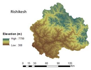
5366             A. K. Shukla et al.: Spatio-temporal assessment of annual water balance models for upper Ganga Basin

Figure 6. Water yield obtained by computing pixel-wise value of parameter w from Xu et al. (2013).

relationship between basin characteristics and the value of           tain the positive value of reference evapotranspiration, as also
parameter w, especially in the case of basin-area character-          suggested by Goyal and Khan (2017). Reference evapotran-
istics. Moreover, no definite relationship has been yet identi-       spiration when multiplied with Kc gives the potential evapo-
fied between basin characteristics and model parameters, and          transpiration. All monthly values are added up to obtain the
this is a subject matter for further study.                           annual value of reference evapotranspiration. Kc is a function
                                                                      of land use and land cover; thus, supervised classification is
                                                                      done to prepare the raster map of land use and land cover
6   Discussion                                                        for the upper Ganga Basin. Subsequently, the annual value
                                                                      of potential evapotranspiration is obtained for the study area
The study aimed to apply the InVEST water yield model                 for the years 1980, 1990, 2001 and 2015.
to compute the water yield for upper Ganga Basin hav-                    The paper employs various methodologies for water yield
ing highly variable topography consisting of hilly, plain and         estimation, as discussed in the methodology section for the
snow-covered areas. The InVEST model is based on the                  upper Ganga Basin. Thus, water yield is computed both from
Budyko theory, which requires low amounts of data and low             the InVEST model as well as the Lumped Zhang model. The
levels of expertise, thus making it acceptable worldwide. The         value of the parameter w is computed using four different
mean monthly precipitation, temperature, monthly value of             approaches, i.e., the mean single value obtained from Xu et
difference of the mean daily maximum and mean daily min-              al. (2013) for large basins, mean single value obtained from
imum, and extraterrestrial radiation parameters for the upper         Xu et al. (2013) for the global model, pixel-level estimated
Ganga Basin of all 4 years, i.e., 1980, 1990, 2001 and 2015,          value of parameter w from Xu et al. (2013) and pixel-wise
are converted into the raster format for various analyses. The        value of parameter w from Donohue et al. (2012). Although
monthly reference evapotranspiration is thus computed us-             the upper Ganga Basin lies in large basin category as per the
ing input parameters in GIS environment by applying the               definition from Xu et al. (2013), the yield computed using
modified Hargreaves equation for all the months, except for           global model is in good agreement with the observed data for
a few months in which the modified Hargreaves equation                the region. In the study, the pixel-level estimation of parame-
gives negative results for the reference evapotranspiration.          ter w is made in order to incorporate the spatial variability of
For those months, the Hargreaves method is applied to ob-             the parameter involved in water yield estimation. Thus, two

Hydrol. Earth Syst. Sci., 22, 5357–5371, 2018                                        www.hydrol-earth-syst-sci.net/22/5357/2018/
A. K. Shukla et al.: Spatio-temporal assessment of annual water balance models for upper Ganga Basin 5367 Figure 7. Water yield obtained by computing pixel-wise value of parameter “w” from Donohue et al. (2012). Figure 8. Spatial distribution of AET obtained from GLDAS Noah output datasets. pixel-wise values of parameter w are computed for the upper lumped water yield is computed using Lumped Zhang model, Ganga Basin for years 1980, 1990, 2001 and 2015 by con- which considers the single mean values for entire basin of all sidering two approaches given by Xu et al. (2013) and the the parameters involved in the computation of water yield. approach given by Donohue et al. (2012). Also, the basin- www.hydrol-earth-syst-sci.net/22/5357/2018/ Hydrol. Earth Syst. Sci., 22, 5357–5371, 2018
5368             A. K. Shukla et al.: Spatio-temporal assessment of annual water balance models for upper Ganga Basin

Figure 9. Spatial distribution of PET obtained from CRU datasets.

                                                                    seasonality, etc. (Li et al., 2013). Again, the factors affecting
                                                                    model parameters vary both spatially and temporally. More-
                                                                    over, the relationship between these factors and model pa-
                                                                    rameters are not yet well defined (Ahn and Merwade, 2017).
                                                                    In such scenarios, adopting a hypothesis by assuming either
                                                                    of these controlling factors (such as “w”) to be spatially or
                                                                    temporally constant is inappropriate. Considering these facts,
                                                                    the present study attempts to incorporate the spatial variabil-
                                                                    ity of model parameter for estimation of water yield at the
                                                                    pixel level. As the computations are made at pixel level (on
                                                                    a grid of size 30 m × 30 m), the assumption of dependence
                                                                    of model parameters on the size of the catchment may also
                                                                    be disregarded. The computations made in the present work
Figure 10. Graphical representation of sub-basin Rishikesh.         are based on empirical equations; however, the application
                                                                    of these equations has been well documented worldwide for
                                                                    estimations of various water balance components at various
                                                                    basin scales (Zhang et al., 2008; Ma et al., 2008; Ning et al.,
The water yield is computed in five different ways for the          2017; Rouholahnejad Freund and Kirchner, 2017; Wang and
upper Ganga Basin for the years 1980, 1990, 2001 and 2015.          Zhou, 2016). Hence, it is recommended that for such a large
   At the Rishikesh gauging site, surface runoff data are ob-       basin, it is required to compute all the parameters involved in
tained by extracting the snowmelt from the discharge data, as       the computations of water yield at the pixel scale rather than
the melting snow contributes about 32 % of total runoff in the      adopting mean values for entire watershed.
Himalayan basins (Maurya et al., 2011). For validating the
water yield obtained from different strategies, the observed
yield is compared with the computed water yield based on            7   Summary and conclusions
different proposed strategies for the years 1980, 1990, 2001
and 2015, as represented in Table 3. The results obtained           The present study aimed to apply the InVEST annual water
from Donohue et al. (2012) and Xu et al. (2013) are com-            yield model, a tool that is gaining interest in the ecosystem
puted at pixel level (Strategy C–E); thus, they exhibit better      services community, in the upper Ganga Basin. While such
performance than other approaches and are in good agree-            simple models have low requirements for data and level of
ment with the observed data. These results exhibit the superi-      expertise, practical applications of such a model with single
ority of pixel-level computation to hydrological analyses for       representative values of the model parameter for the entire
a watershed. The parameters involved in the Budyko model            basin do not provide accurate estimates of water yield. Per-
are dependent on various factors, such as basin character-          forming pixel scale computation of water yield in the study
istics (size, topography, stream length, slope, etc.), climate      indicates a better performance, and the results obtained show

Hydrol. Earth Syst. Sci., 22, 5357–5371, 2018                                     www.hydrol-earth-syst-sci.net/22/5357/2018/
A. K. Shukla et al.: Spatio-temporal assessment of annual water balance models for upper Ganga Basin 5369
better agreement with the observed water yield. As far as pa- Author contributions. AKP assisted with data collection, data pro-
rameter w is concerned, the global model works better than cessing and data analysis; SP with data analysis and writing, the
other representations of parameter w available in literature, analysis of results, and the review, revision and proofreading of the
especially in the upper Ganga Basin. In the study, the water paper; LP with data analysis and writing, the analysis of results,
yield is computed using five different strategies, and results and the review, revision and proofreading the paper; CSPO with
the analysis of results and the review, revision, and supervision of
are validated with the observed data at the outlet of the upper
the whole work and proofread the paper; AM supervised the whole
Ganga Basin. The present study attempts to quantify annual work; and RDG assisted with the review, revision and supervision
water yield at the pixel level, making the computations in- of the whole work.
dependent of the size of catchment. Therefore, the proposed
methodology is expected to perform well for a catchment of
any given size. Changes in catchment water storage over time Competing interests. The authors declare that they have no conflict
are required to be quantified in order to validate the applica- of interest.
bility of Budyko’s model to long-term data for the studied
catchment. Earlier, some of the important parameters defin-
ing water yield used to be computed at a basin-level scale, Special issue statement. This article is part of the special issue
which caused errors in the results. “The changing water cycle of the Indo–Gangetic Plain”. It does not
The study attempts to incorporate the spatial variability of belong to a conference.
parameters involved in the model through the pixel-level es-
timation of parameters that are otherwise taken as lumped in
the previous studies. Study results show that the estimated Acknowledgements. Authors are thankful to the executive engineer
water yield, considering spatial variability in model param- of the Irrigation Department of Uttarakhand for providing the
eters, is in better agreement with the observed water yield discharge data for the Rishikesh sub-basin of upper Ganga Basin.
compared to the water yield estimated when considering the
Edited by: Pradeep P. Mujumdar
parameters to be lumped over the study region. Further, the Reviewed by: two anonymous referees
computations of various parameters are made at the pixel
level; therefore, the estimates of water balance components
using this approach are expected to be independent of the
assumption of dependence of parameters on catchment size. References
As the relationship between Budyko’s model parameters and Ahn, K. H. and Merwade, V.: The Integrated Impact of Basin Char-
their controlling factors has not been well defined (Ahn and acteristics on Changes in Hydrological Variables, in: chap. 12 in
Merwade, 2017), the study emphasizes water yield estima- “Sustainable Water Resources Management”, American Society
tion using pixel-based computations. The study outcomes of Civil Engineers (ASCE), Virginia, USA, 317–336, 2017.
can be summarized as follows: (i) between two approaches Allen, R. G., Pereira, L. S., Raes, D., and Smith, M.: Crop evap-
used in the study, i.e., considering the entire basin and pixel- otranspiration – Guidelines for computing crop water require-
level approach, the pixel-level approach is found to provide ments, FAO Irrigation and drainage paper 56, FAO, Rome, 300,
better results; and (ii) in pixel-based computations, results D05109, 1998.
are further improved with the use of a parameter w based on Bai, Y., Ouyang, Y., and Pang, J. S.: Biofuel supply chain design un-
der competitive agricultural land use and feedstock market equi-
a global model rather than regional models of parameter w,
librium, Energy Econ., 34, 1623–1633, 2012.
especially for large basins in the Himalayan region.
Bharati, L., Lacombe, G., Gurung, P., Jayakody, P., Hoanh, C. T.,
and Smakhtin, V.: The impacts of water infrastructure and cli-
mate change on the hydrology of the Upper Ganges River Basin,
Data availability. The meteorological data products are provided in: Vol. 142, IWMI, Colombo, Sri Lanka, 2011.
by the Indian Meteorological Department on the basis of pay- Budyko, M. I.: The Heat Balance of the Earth, Leningrad, 1956,
ment. It can be purchased from the following URL: http://www. Translation by N. A. Stepanova, US Weather Bureau, Washing-
imdpune.gov.in/ndc_new/Request.html (India Meteorological De- ton, 1–254, 1958.
partment, 2018). The hydrological data in upper Ganga basin is pro- Budyko, M. I.: Climate and Life, Academic Press, New York, USA,
vided by the Uttarakhand Irrigation Department, which is available 1–507, 1974.
for research purposes only. Satellite datasets are acquired from the Budyko, M. I. and Ronov, A. B.: Evolution of chemical composition
USGS web portal (https://earthexplorer.usgs.gov/, Earth Explorer – of the atmosphere during the Phanerozoic, Geokhimiya, 5, 643–
USGS, 2018). The soil maps are provided by the National Bureau of 653, 1979.
Soil Survey and Land Use Planning, India on the basis of payment Choudhury, B.: Evaluation of an empirical equation for annual
from the following URL: https://www.nbsslup.in/publications.html evaporation using field observations and results from a biophys-
(ICAR, 2018). ical model, J. Hydrol., 216, 99–110, 1999.
Donohue, R. J., Roderick, M. L., and McVicar, T. R.: Roots, storms
and soil pores: Incorporating key ecohydrological processes into
Budyko’s hydrological model, J. Hydrol., 436, 35–50, 2012.
www.hydrol-earth-syst-sci.net/22/5357/2018/ Hydrol. Earth Syst. Sci., 22, 5357–5371, 20185370 A. K. Shukla et al.: Spatio-temporal assessment of annual water balance models for upper Ganga Basin
Droogers, P. and Allen, R. G.: Estimating reference evapotranspi- Ning, T., Li, Z., and Liu, W.: Vegetation dynamics and climate sea-
ration under inaccurate data conditions, Irrig. Drain. Syst., 16, sonality jointly control the interannual catchment water balance
33–45, 2002. in the Loess Plateau under the Budyko framework, Hydrol. Earth
Earth Explorer – USGS: available at: https://earthexplorer.usgs. Syst. Sci., 21, 1515–1526, https://doi.org/10.5194/hess-21-1515-
gov/, last access: 15 September 2018. 2017, 2017.
Fu, B. P.: On the calculation of the evaporation from land surface, Ojha, C. S. P., Bhunya, P., and Berndtsson, R.: Engineering Hy-
Sci. Atmos. Sin., 5, 23–31, 1981. drology, 1st Edn., Oxford University Press, Oxford, UK, 1–459,
Goyal, M. K. and Khan, M.: Assessment of spatially explicit annual 2008.
water-balance model for Sutlej River Basin in eastern Himalayas Ol’Dekop, E. M.: On Evaporation from the Surface of River Basins,
and Tungabhadra River Basin in peninsular India, Hydrol. Res., Univ. of Tartu, Tartu, Estonia, 1–208, 1911.
48, 542–558, 2017. Pai, D. S., Sridhar, L., Rajeevan, M., Sreejith, O. P., Satbhai, N.
Guswa, A. J., Brauman, K. A., Brown, C., Hamel, P., Keeler, B. L., S., and Mukhopadhyay, B.: Development of a new high spatial
and Sayre, S. S.: Ecosystem services: Challenges and opportuni- resolution (0.25 × 0.25) long period (1901–2010) daily gridded
ties for hydrologic modeling to support decision making, Water rainfall data set over India and its comparison with existing data
Resour. Res., 50, 4535–4544, 2014. sets over the region, Mausam, 65, 1–18, 2014.
Hamel, P. and Guswa, A. J.: Uncertainty analysis of a spatially ex- Pathak, S., Ojha, C. S. P., Zevenbergen, C., and Garg, R. D.: Rank-
plicit annual water-balance model: case study of the Cape Fear ing of Storm Water Harvesting Sites Using Heuristic and Non-
basin, North Carolina, Hydrol. Earth Syst. Sci., 19, 839–853, Heuristic Weighing Approaches, Water, 9, 710, 2017.
https://doi.org/10.5194/hess-19-839-2015, 2015. Pike, J. G.: The estimation of annual run-off from meteorological
Hoyer, R. and Chang, H.: Assessment of freshwater ecosystem ser- data in a tropical climate, J. Hydrol., 2, 116–123, 1964.
vices in the Tualatin and Yamhill basins under climate change Porporato, A., Daly, E., and Rodriguez-Iturbe, I.: Soil water balance
and urbanization, Appl. Geogr., 53, 402–416, 2014. and ecosystem response to climate change, Am. Nat., 164, 625–
India Meteorological Department: available at: http://www. 632, 2004.
imdpune.gov.in/ndc_new/Request.html, last access: 10 Octo- Redhead, J. W., Stratford, C., Sharps, K., Jones, L., Ziv, G., Clarke,
ber 2018. D., Oliver, T. H., and Bullock, J. M.: Empirical validation of the
ICAR: ICAR-NBSS&LUP Publications 2012–17, available at: InVEST water yield ecosystem service model at a national scale,
https://www.nbsslup.in/publications.html, last access: Octo- Sci. Total Environ., 569, 1418–1426, 2016.
ber 2018. Rouholahnejad Freund, E. and Kirchner, J. W.: A Budyko frame-
Khatami, S. and Khazaei, B.: Benefits of GIS Application in Hydro- work for estimating how spatial heterogeneity and lateral mois-
logical Modeling: A Brief summary, VATTEN – J. Water Man- ture redistribution affect average evapotranspiration rates as seen
age. Res., 70, 41–49, 2014. from the atmosphere, Hydrol. Earth Syst. Sci., 21, 217–233,
Li, D., Pan, M., Cong, Z., Zhang, L., and Wood, E.: Vegetation con- https://doi.org/10.5194/hess-21-217-2017, 2017.
trol on water and energy balance within the Budyko framework, Sánchez-Canales, M., Benito, A. L., Passuello, A., Terrado, M., Ziv,
Water Resour. Res., 49, 969–976, 2013. G., Acuña, V., Schuhmacher, M., and Elorza, F. J.: Sensitivity
Ma, Z. M., Kang, S. Z., Zhang, L., Tong, L., and Su, X. L.: Analysis analysis of ecosystem service valuation in a Mediterranean wa-
of impacts of climate variability and human activity on stream- tershed, Sci. Total Environ., 440, 140–153, 2012.
flow for a river basin in arid region of northwest China, J. Hy- Schreiber, P.: Über die Beziehungen zwischen dem Niederschlag
drol., 352, 239–249, 2008. und der Wasserführung der Flüsse in Mitteleuropa, Z. Meteorol.,
Maurya, A. S., Shah, M., Deshpande, R. D., Bhardwaj, R. M., 21, 441–452, 1904.
Prasad, A., and Gupta, S. K.: Hydrograph separation and pre- Srivastava, A. K., Rajeevan, M., and Kshirsagar, S. R.: Development
cipitation source identification using stable water isotopes and of a high resolution daily gridded temperature data set (1969–
conductivity: River Ganga at Himalayan foothills, Hydrol. Pro- 2005) for the Indian region, Atmos. Sci. Lett., 10, 249–254,
cess., 25, 1521–1530, 2011. 2009.
McKenzie, N. J., Gallant, J., and Gregory, L.: Estimating wa- Su, C. and Fu, B.: Evolution of ecosystem services in the Chi-
ter storage capacities in soil at catchment scales, CRC for nese Loess Plateau under climatic and land use changes, Global
Catchment Hydrology, CRC Publications, Monash University, Planet. Change, 101, 119–128, 2013.
Monash, Australia, 2003. Tallis, H. T., Ricketts, T., Nelson, E., Ennaanay, D., Wolny, S., Ol-
Mezentsev, V.: More on the computation of total evaporation (Ye- wero, N., Vigerstol, K., Pennington, D., Mendoza, G., Aukema,
chio raz o rastchetie srednevo summarnovo ispareniia), Mete- J., and Foster, J.: InVEST 1.004 beta User’s Guide, The Nat-
orog. i Gridrolog., 5, 24–26, 1955. ural Capital Project, Stanford University, USA, available at:
Milly, P. C. D. and Dunne, K. A.: Macroscale water fluxes 2. Water https://naturalcapitalproject.stanford.edu/invest/ (last access: Oc-
and energy supply control of their interannual variability, Water tober 2018), 2010.
Resour. Res., 38, 241–249, 2002. Terrado, M., Acuña, V., Ennaanay, D., Tallis, H., and Sabater, S.:
Nelson, E., Sander, H., Hawthorne, P., Conte, M., Ennaanay, Impact of climate extremes on hydrological ecosystem services
D., Wolny, S., Manson, S., and Polasky, S.: Projecting global in a heavily humanized Mediterranean basin, Ecol. Indic., 37,
land-use change and its effect on ecosystem service provision 199–209, 2014.
and biodiversity with simple models, PloS One, 5, E14327, Turc, L.: Le bilan d’eau des sols: relations entre les précipitations,
https://doi.org/10.1371/journal.pone.0014327, 2010. l’évaporation et l’écoulement, Annales Agronomiques A, 20,
491–595, 1954.
Hydrol. Earth Syst. Sci., 22, 5357–5371, 2018 www.hydrol-earth-syst-sci.net/22/5357/2018/A. K. Shukla et al.: Spatio-temporal assessment of annual water balance models for upper Ganga Basin 5371 Wang, D. and Tang, Y.: A one-parameter Budyko model for wa- Zhang, L., Hickel, K., Dawes, W. R., Chiew, F. H., Western, A. ter balance captures emergent behavior in darwinian hydrologic W., and Briggs, P. R.: A rational function approach for esti- models, Geophys. Res. Lett., 41, 4569–4577, 2014. mating mean annual evapotranspiration, Water Resour. Res., 40, Wang, X.-S. and Zhou, Y.: Shift of annual water balance in W02502, https://doi.org/10.1029/2003WR002710, 2004. the Budyko space for catchments with groundwater-dependent Zhang, L., Potter, N., Hickel, K., Zhang, Y. Q., and Shao, Q. X.: evapotranspiration, Hydrol. Earth Syst. Sci., 20, 3673–3690, Water balance modeling over variable time scales based on the https://doi.org/10.5194/hess-20-3673-2016, 2016. Budyko framework – Model development and testing, J. Hydrol., Xu, X., Liu, W., Scanlon, B. R., Zhang, L., and Pan, M.: Local 360, 117–131, 2008. and global factors controlling water-energy balances within the Zhou, G., Wei, X., Chen, X., Zhou, P., Liu, X., Xiao, Y., Sun, G., Budyko framework, Geophys. Res. Lett., 40, 6123–6129, 2013. Scott, D. F., Zhou, S., Han, L., and Su, Y.: Global pattern for the Yang, D., Sun, F., Liu, Z., Cong, Z., Ni, G., and Lei, effect of climate and land cover on water yield, Nat. Commun., Z.: Analyzing spatial and temporal variability of annual 6, 5918, https://doi.org/10.1038/ncomms6918, 2015. water-energy balance in nonhumid regions of China using Zhou, S., Yu, B., Huang, Y., and Wang, G.: The complementary the Budyko hypothesis, Water Resour. Res., 43, W04426, relationship and generation of the Budyko functions, Geophys. https://doi.org/10.1029/2006WR005224, 2007. Res. Lett., 42, 1781–1790, 2015. Yang, H., Yang, D., Lei, Z., and Sun, F.: New ana- Zhou, X., Zhang, Y., Wang, Y., Zhang, H., Vaze, J., Zhang, L., Yang, lytical derivation of the mean annual water-energy Y., and Zhou, Y.: Benchmarking global land surface models balance equation, Water Resour. Res., 44, W03410, against the observed mean annual runoff from 150 large basins, https://doi.org/10.1029/2007WR006135, 2008. J. Hydrol., 470, 269–279, 2012. Zhang, L., Dawes, W. R., and Walker, G. R.: Response of mean an- nual evapotranspiration to vegetation changes at catchment scale, Water Resour. Res., 37, 701–708, 2001. www.hydrol-earth-syst-sci.net/22/5357/2018/ Hydrol. Earth Syst. Sci., 22, 5357–5371, 2018
You can also read