Graduated Flood Risks and Property Prices in Galveston County
←
→
Page content transcription
If your browser does not render page correctly, please read the page content below
Graduated Flood Risks and Property Prices in
              Galveston County

            Ajita Atreya                          Jeffrey Czajkowski
        Wharton Risk Center                       Wharton Risk Center
      University of Pennsylvania                University of Pennsylvania

                                  July 1, 2015
                             Working Paper # 2015-09

_____________________________________________________________________
               Risk Management and Decision Processes Center
               The Wharton School, University of Pennsylvania
              3730 Walnut Street, Jon Huntsman Hall, Suite 500
                          Philadelphia, PA, 19104
                                    USA
                           Phone: 215‐898‐5688
                            Fax: 215‐573‐2130
                    http://www.wharton.upenn.edu/riskcenter
___________________________________________________________________________
THE WHARTON RISK MANAGEMENT AND DECISION PROCESSES CENTER
       Established in 1984, the Wharton Risk Management and Decision Processes
Center develops and promotes effective corporate and public policies for low‐probability
events with potentially catastrophic consequences through the integration of risk
assessment, and risk perception with risk management strategies. Natural disasters,
technological hazards, and national and international security issues (e.g., terrorism risk
insurance markets, protection of critical infrastructure, global security) are among the
extreme events that are the focus of the Center’s research.
        The Risk Center’s neutrality allows it to undertake large‐scale projects in
conjunction with other researchers and organizations in the public and private sectors.
Building on the disciplines of economics, decision sciences, finance, insurance, marketing
and psychology, the Center supports and undertakes field and experimental studies of
risk and uncertainty to better understand how individuals and organizations make
choices under conditions of risk and uncertainty. Risk Center research also investigates
the effectiveness of strategies such as risk communication, information sharing, incentive
systems, insurance, regulation and public‐private collaborations at a national and
international scale. From these findings, the Wharton Risk Center’s research team – over
50 faculty, fellows and doctoral students – is able to design new approaches to enable
individuals and organizations to make better decisions regarding risk under various
regulatory and market conditions.
       The Center is also concerned with training leading decision makers. It actively
engages multiple viewpoints, including top‐level representatives from industry,
government, international organizations, interest groups and academics through its
research and policy publications, and through sponsored seminars, roundtables and
forums.
       More information is available at http://wharton.upenn.edu/riskcenter
       .
Graduated Flood Risks and Property Prices in Galveston County

                                             Abstract
A number of hedonic property pricing studies of flood risk indicate that properties within a
designated higher flood risk zone sell for a lower price than an equivalent property outside of it.
However, often the homes most at flood risk are also the most desirable in terms of their proximity
to the water, and this concurrent existence of positive water-related amenities and negative flood
risk may be problematic to parse out in a hedonic estimation. Our hedonic property analysis
approach in Galveston County, Texas aims at estimating the impacts of flood risk and water-related
amenities in a more systematic way by interacting distance to the nearest coastline and flood risk
in order to account for these impacts acting together on housing sales prices in our coastal
community. Further, we employ a more granular view of the flood risk split by varying flood risk
return periods to allow for a more meaningful interaction between the negative and positive
amenities related to proximity to the water. Results show that the hedonic price effect is dependent
upon the distance to the nearest coastline, and as expected the distance effect varies by flood risk
type. We find that in this coastal housing market properties located in the highest risk flood area,
for up to nearly a quarter mile from the nearest coastline, actually command a price premium. A
recent movement toward risk-based flood insurance premiums in the United States was deeply
opposed by the real estate sector for fear of causing property values to steeply decline. This
analysis sheds some further light on this depressed property value assertion highlighting its
sensitivity to distance to the water.

Key words: hedonic housing prices, flood risk, return periods, water amenity, Galveston Texas,

                                                 1
I.      Introduction

Since 1968 homeowners’ flood insurance in the United States has been mainly provided through

the federally-run National Flood Insurance Program (NFIP), which as of 2014 has 5.34 million

NFIP policies-in-force nationwide with a total of $1.27 trillion of insured coverage (FEMA, 2014).

To set premiums, the NFIP maps participating communities via Flood Insurance Rate Maps

(FIRMs), designating flood risks through different flood zones. A number of hedonic property

pricing studies of flood risk indicate that properties within a designated higher flood risk zone sell

for a lower price than an equivalent property outside of it, typically on the order of 4 to 12 percent

(Bin and Polasky 2004; Bin, et al. 2008a; Kousky 2010; Posey and Rogers, 2010; Bin and Landry

2012). This negative flood risk price differential is characteristically attributed to higher flood

insurance rates (the discounted sum of future flood insurance payments) being capitalized into

housing sales prices in the higher flood risk zones (Bin et al. 2008a; Bin and Landry 2012).1

        However, an estimated hedonic price discount for location in a higher flood risk zone does

not always hold (USACE, 1998; Bin and Kruse, 2006; Morgan, 2007; Daniel et al., 2009). For

example, Daniel et al. (2009) in their meta-analysis of 19 studies and 117 point estimates of the

implicit price for location in the 100 year flood plain find that the estimates vary considerably,

anywhere from -52% to +58%. Furthermore, with any estimated hedonic flood risk price

differential two complications potentially arise (Daniel et al. 2009): subjective bias of the objective

flood risk including a complete lack of awareness of the risk; and the concurrent existence of

positive water-related amenities and negative flood risk inherent in living near to the water. In this

study in addition to using the traditional flood zones as a measure of objective flood risk we

incorporate a more comprehensive measure of flood risk through identified flood return periods

                                                  2
and aim to determine if the potential effects of higher flood risks is offset by coastal amenities

conferred on a property from being located close to water using hedonic property analysis. We

allow for the flood risk and the coastal amenity to act jointly on housing sales price in Galveston

County, a coastal community in Texas. . As other studies (Kousky 2010; Bin and Landry 2012;

and Atreya et. al. 2013 ) find no evidence of flood risk impacting housing prices until the

occurrence of a major event we also demonstrate the robustness of our results to the potential

subjective bias associated with the occurrence of Hurricane Ike in 2008 which made landfall in

Galveston. 2

       Often the homes most at flood risk are also the most desirable in terms of their proximity

to the water. Hence, by only capturing the location of a home in or outside of the floodplain

through an indicator variable in the hedonic estimation (where 1= location within the high risk

floodplain such as whether a property lies in the 100 or 500 year return periods, and 0 = location

outside of it) may bias the estimation of flood risk. Bin et al. (2008a) and Daniel et al. (2009)

explicitly discuss the importance of controlling for the positive amenity values related to water

proximity, and utilize distance measures of proximity to the water in their estimations. Others also

control for positive water-related amenities through distance measures in their hedonic flood risk

studies (Kousky, 2010; Conroy and Milosch, 2011; Bin and Landry 2012; Atreya et al., 2013). 3

Although the distance to water measure is incorporated to account for the positive water amenity

effects, these studies do not vary the amenity effects by flood risk type in their estimations. In

other words, any change in distance to or from the water has an analogous impact across high to

low flood risk types. But intuitively this risk-amenity trade-off would seem to vary by flood risk

type, where a high flood risk area would be penalized more for the loss of the positive amenity

given that the high flood risk remains. Here we capture these distance varying risk-amenity trade-

                                                 3
offs through interaction terms of flood risk and distance that have rarely been employed to our
knowledge.4
Regardless of controlling for water-related positive amenity values, the hedonic literature’s
inconclusiveness concerning a home price discount stemming from a negative flood risk may be
partially attributed to the tendency to capture flood risk in the empirical analysis through the use
of the aforementioned indicator dummy variable where 1= location within the high risk floodplain,
and 0 = location outside of it (Bin and Polasky 2004; Bin and Kruse 2006; Morgan, 2007; Bin et
al. 2008a; Kousky 2010; Posey and Rogers, 2010; Bin and Landry 2012; Atreya et al., 2013). This
dummy indicator structure implies that the hedonic price flood risk discount is constant across the
floodplain (USACE, 1998) despite the fact that the flood risk clearly is not. For example, within
an identified 100-year flood zone the flood risk can vary from a 10 year return period (10%
probability of occurrence in any given year) to a 100 year return period (1% probability of
occurrence in any given year). And NFIP insurance premiums also vary within a particular
aggregate flood zone via the elevation of the first floor of the dwelling in relation to the 100-year
return period, indicating hedonic price discounts (capitalized insurance payments) should vary by
varying risk within a flood zone. Czajkowski et al. (2013) and Michel-Kerjan et al. (2014) use
flood catastrophe models in two Texas communities – including Galveston County - to show not
only how much flood risk varies within a single NFIP designated flood risk zone, but by how much
corresponding non-NFIP probabilistically derived localized risk-based flood insurance rates would
vary as well.5
In order to capture this inherent varying flood risk within a given flood map zone Griffith
(1994) included a flood frequency (i.e., return period) variable in her analysis and found that there
is a hedonic price discount only for those homes deep in the 100 year floodplain due to their higher
4annual probability of occurrence. A number of other studies have utilized measures of elevation
or flood depth in lieu of, or in addition to, a flood risk zone indicator variable to account for the
spatially inherent varying flood risk (Barnard, 1978; Tobin and Montz, 1994; Kriesel and
Friedman, 2002; Zhai et al., 2003; Kousky, 2010; McKenzie and Levendis, 2010; and Atreya et
al., 2013), and typically find a statistically significant relationship in the hedonic estimation.
However, often the employed measure of elevation does not necessarily best convey the flood risk
which would be relative to the base flood elevation, i.e., the computed elevation to which
floodwater is anticipated to rise during the flood having a one percent chance of being equaled or
exceeded in any given year (FEMA, 2014). For example, McKenzie and Levendis (2010) utilize
elevation in relation to the mean sea-level, whereas Kousky (2010) and Atreya et al. (2013) simply
control for the elevation of the ground, not in relation to the base flood elevation level. Here in
addition to using the traditional flood zone indicator dummy variables, we utilize data provided to
us by CoreLogic, a large real estate data provider that identifies the varying flood risk return
periods within the classified FIRM flood zones.
Overall then, our hedonic property analysis approach in Galveston County, Texas aims to
determine countervailing impacts of flood risk and water-related amenities in a more systematic
way than has previously been employed (Daniel et al., 2009). We first control for positive
amenities associated with water proximity by using spatial analysis in Arc-GIS to calculate for
each property their distance to the nearest coastline. We then interact distance and flood risk in our
hedonic estimations in order to account for these impacts acting together on housing sales prices
in our coastal community. Finally we employ a more granular view of flood risk split by varying
flood risk return periods to allow for a more meaningful interaction between the negative and
positive amenities related to proximity to the water than would otherwise be achieved with an
5aggregate flood zone indicator variable. We feel it is reasonable to believe that homeowners in a
100 year floodplain are able to discern the varying levels of flood risk within a particular flood
zone, especially in a frequently flooded area such as Galveston County. This belief is further
supported by the statistical significance of elevation or flood depth variables utilized in the existing
hedonic literature already cited.
Our results show that properties located in the high risk flood areas command a price
premium compared to those located outside. But this hedonic price premium is dependent upon
the distance to the coast, and as expected the distance effect varies by flood risk type. This
illustrates the importance of capturing these two variables acting together through the interaction
terms, otherwise the flood risk is misestimated. We show that the misestimation is more
pronounced when we utilize a more granular flood risk and distance interaction with the varying
return period risk information inherent to each zone, highlighting the need for using more detailed
risk information when available. Overall, we find that properties located in the highest risk flood
area, for up to nearly a quarter mile from the nearest coastline, actually command a price premium.
Importantly results are also robust to the potential subjective bias associated with the occurrence
of Hurricane Ike in 2008.
In 2012, Congress passed the Biggert-Waters Flood Insurance Reform Act (BW-12) in
order to address a number of the well-documented structural and fiscal issues of the program,
including key provisions of the bill that would increase existing discounted premiums to full-risk
levels. However, BW-12 was itself reformed in March 2014 with the passage of Homeowner
Flood Insurance Affordability Act (HFIAA-14) that importantly curbed many of the planned BW-
12 rate increases. Realtors, homebuilders, and lenders had provided steep opposition to BW-12
(WSJ, 2013) decrying the movement toward risk-based premiums as causing “property values to
6steeply decline and made many homes unsellable, hurting the real estate market” (Insurance
Journal, March 2014). Importantly, our results shed some further light on this depressed property
value assertion highlighting the sensitivity of the assertion as being dependent upon the sufficient
disentanglement of the coincident flood risk and water amenity effects. That is, even despite our
systematic interaction approach coupled with more detailed flood risk data, we find that in the
absence of a significant flood event it is difficult for the negative flood amenity value based upon
the objective flood risk to sufficiently counteract a homeowner’s strong desire to live near the
water. The remainder of the paper proceeds as follows: section two provides an overview of the
Galveston County study area as well as the details of the data utilized in our hedonic analysis;
section three lays out the methods we employ while the corresponding main results are presented
in section four; robustness of these results are presented in section five; and finally section six
concludes.
II. Study Area and Data
We focus our study in Galveston County, Texas exposed to both riverine and storm-surge flooding.
Property transaction data for single family homes in Galveston County was provided by
CoreLogic. After cleaning the dataset6 we retained 35,586 property sales for our analysis between
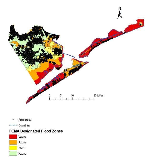
the years 2001 and 2010, including only the most recent sale in the analysis. Figure 1 illustrates
the location of these sales by our aggregated FEMA designated flood zones V, A, X500, and X. 7
V and A zones represent high risk - 1 percent or greater annual chance of flooding – in coastal and
non-coastal areas respectively. Whereas X500/B and X/C zones represent moderate to minimal
flood risk areas.
While the number of sales in any one year is largest in the X/C zone, i.e., minimal flood
risk areas, on average there were 381 sales per year in the high risk flood areas (V and A zones)
7and 627 home sales per year in the moderate flood risk area (X500/B) during this timeframe
(Figure 2). We adjusted all sales prices to 2010 values utilizing the housing price index for
Houston–The Woodlands-Sugar Land, Texas metropolitan statistical area from the office of
Federal Housing Finance Agency (FHFA, 2014). In a coastal community such as Galveston, an
important amenity measure that affects the property price is proximity to nearest coastline (Bin et
al., 2008a; Daniel et al. 2009). Using spatial analysis in Arc-GIS we calculated for each property
their Euclidean distance to the nearest coastline. As would be expected given their relative
proximity to the coastal waterfront as shown in Figure 1 above (and from Table I), homes in the
V and A zones sell for more on average after accounting for the size of the home with sales prices
per square foot of $198.51, $115.92, $86.72, and $92.75 for the V, A, X500/B, and X/C zones
respectively.
However, while homes located in V and A zones are in the aggregate relatively closer to
the water as compared to those located in X500 and X zones (approximately 98 and 66 percent of
V and A zone homes sales are within 1 mile of the nearest coastline as compared to 31 and 3
percent of X/500 and X zone home sales), there is still a significant amount of variation of distance
to the nearest coast within each zone. Figure 3 provides the average sales price per square foot
split by distance to the nearest coastline in 500 to 1000 foot increments overlaid with an A zone
linear trendline. From this view of our sales price data we see that each flood zone has homes
relatively close the water, but as distance from the nearest coastline increases, sales price per
square foot within each flood zone generally declines as expected.
Furthermore, not only does the distance to the nearest coastline vary within a flood zone,
i.e., the positive amenity value, but so does the negative amenity flood risk value vary within an
aggregated zone. CoreLogic determines the associated relative flood risk (i.e., flood return
8periods) for each home based upon a proprietary scoring of a property’s elevation variance (EV)
and distance to the most immediate water flood hazard. Where EV is the difference between the
elevation of the ground upon which the immediate structure rests and the elevation of the flood
plain that presents the greatest flood risk such as the base flood elevation for homes in the A zone.
The specific discretized flood return periods (RPs) determined by CoreLogic that we use for our
hedonic analysis are: RP ≤ 10; 10 < RP ≤ 25; 25 < RP ≤ 50; 50 < RP ≤ 100; 100 < RP ≤ 250; 250
< RP ≤ 500; 500 < RP ≤ 1000; 1000 < RP ≤ 5000; and RP > 5000.
As an example of just how much the RPs vary within a particular flood zone, we highlight
the distribution of the Galveston County A zone home sales by the various return periods within
this 100 year flood zone. While all of these homes are located within the 100 year flood plain
equating to a 1 percent annual chance flood event, some of these homes are at a higher risk of
flooding based upon their individual location within the zone. For example, homes subject to at
least a 10 percent chance of a flood event, or a 10 year return period comprise 14 percent of the
total sales from 2001 to 2010. Overall, nearly 80 percent of the home sales from 2001 to 2010
were at a 50 year return period or less (10 < RP ≤ 25 = 37 percent and 25 < RP ≤ 50 = 27 percent).
The V, X500 and X zones have similar varying home sale flood risk (RP) distributions.
We present in Figure 4 sales price per square foot by a combined view of flood risk return
periods up to 100 years and distance to the coast from 0 to 5000 feet. From here we can see that
riskier homes (RP 25 or less) in general have higher prices per square foot compared to less risky
homes across all of the defined distance bands. However, where this difference is greatest is for
homes directly on the water (0 to 500 feet), but the price differences become less as distance to the
coast increases (from Table I we see that homes in RP 25 or less are on average closer to the water,
nearly all within a half a mile distance on average). In fact, we begin to see an uptick in the sales
9price per square foot in the 50 to 100 RP area as the distance to coast increases. Clearly then there
is a variation in price per square foot depending upon the interaction of distance to the nearest
coast and flood risk, or the varying trade-off between positive and negative water-related amenities
dependent upon the particular flood risk.8 And it is precisely this interaction we isolate in our
hedonic framework.
Beyond the square footage of the home, flood risk return period, and distance from the
nearest coastline there are a number of other relevant housing attributes – structural,
location/neighborhood, etc - that consistently impact property sales prices and we include these in
our hedonic framework. Specifically we include the following structural attributes in the estimated
hedonic price functions: land square footage, building square footage, the number of stories,
exterior wall type with brick = 1 and 0 = otherwise (aluminum, asbestos, brick veneer, brick/wood,
concrete, concrete block, frame wood, metal, stone, stucco, tilt-up, wood frame) type of foundation
with slab-on-grade = 1 and 0 = otherwise (wood, concrete, concrete block, pier, pipe/iron) , a
dummy indicator variable for the condition of the home with 1 = excellent and 0 = otherwise (Poor,
Average, Fair, Good, Very Good) and age of the property at the time of sale. In addition to the
distance to the coast we also use spatial analysis in Arc-GIS to calculate for each property their
Euclidean distance to the nearest park, bus route, railroad and school. The demographic
characteristics, such as the median household income and the percent of nonwhite population was
determined at the census tract level using 2000 census data. As properties that are built after a
community joins the NFIP require the lowest floor of the residential building to be elevated above
the base flood elevation, we include a dummy variable, NFIP=1 if the property was built after 1974
(i.e. after the communities in Galveston County joined NFIP) and 0 otherwise. Finally, we include
10another dummy variable seawall=1 if the properties were protected by the Galveston seawall and
0 otherwise.9
Table I provides the summary statistics of the variables used in the analysis. The average
selling price in our sample is $181,690 with a typical home about 20 years old and 2,150 square
feet. About 5.5 percent of the homes sold are located in V zone and 16 percent of the homes sold
are located in A zone. 6 percent of the homes sold are located in the flood return period less than
10 years. On average the distance to coast is 25,694 feet and 2.4 percent of the houses are located
within 500 feet of the coast. 82 percent of the houses in our sample were built after the community
joined NFIP and 11 percent of the houses are protected by seawall. As illustrated earlier, there is
much variation in the price of the properties within the FEMA designated flood zones and the price
variation also depends on the proximity to the coast. We further split the flood zone and return
period by mean price as well as mean coastal distance at the end of Table I. We also present the
average price of the properties split by their distance to the coast.
III. Methods
This study aims at disentangling the countervailing impacts of flood risk and coastal water
amenities as reflected in the property prices in Galveston County TX. We employ hedonic models
(Rosen 1974; Freeman 2003) that have been extensively used in the past to partition out the value
of an environmental amenity or disamenity using the actual property transaction data based on the
notion that the component values of various attributes of heterogeneous goods are reflected in price
differentials. The standard hedonic model can be represented as:
P=f (S, L, R, C). In a hedonic model, price of the property (P) is modeled as a function of its
structural attributes (S) such as building square feet, age, number of bathrooms; location attributes
11(L) such as distance to road, distance to park; and the environmental variables of interest which in
our case is coastal amenity as measured by distance to the nearest coast (C) and flood risk (R).
The first order differentiation of price, (P), with respect to the housing attributes provide the
marginal implicit price which can be interpreted as the marginal willingness to pay for that
attribute. For flood risk (R) we use both the flood zones as given by FEMA’s flood insurance rate
maps as well as a more granular measure of flood risk through specific flood return periods
Use of FEMA designated flood risk zones in hedonic model
First, we incorporate flood risk (R) in our model using traditional FEMA designated flood hazard
zones: the V, A, X500, and X zones. Distance to coast is an important factor that affects the price
of a property (Bin et al. 2008a; Daniel et al. 2009; Kousky, 2010; Conroy and Milosch, 2011; Bin
and Landry 2012; Atreya et al., 2013). To allow the implicit price of coastal amenity to vary
between properties locating in various flood risk zones, the distance to coast variable enters the
hedonic model in three ways. First, in model (1), we include the natural log of distance to the
nearest coastline to capture the diminishing marginal returns as the distance to the coast increases.
The model is as follows:
J K L
log( Pit ) o j S ijt k Likt l Ril m ln(C ) i i t it (1)
j 1 k 1 l 1
where, log(Pit) is the natural log of the price for observation i in time t, Sijt is the jth structural
attribute for observation i in time t, Likt is the kth locational attribute for observation i in time t,
Ril is the lth risk variable for observation i which in our case include dummy variables for V, A
and X500 zones, i.e. incorporates three dummy variables equal to 1 if the property falls within the
designated V, A and X500 zones and 0 otherwise. The properties that fall in X zone are the control
12groups. Ln(C)i is the distance-to-coast variable for observation i. The estimate from the natural
log of coastal distance (C) is an average premium effect measured at the mean.
We expect the effect of distance-to-coast to be non-linear and thus secondly, we construct
distance dummy variables to capture discrete distance effects as follows:
J K L M
log( Pit ) o j S ijt k Likt l Ril m .Cim i t it (2)
j 1 k 1 l 1 m 1
In model (2), variable Cim a dummy variable denoting a specific distance from the coast for each
observation i. The distance dummy variable are adjusted to capture smaller distance effects, i.e.,
within 500 feet, between 500 and 1000 feet, between 1000 and 2000 feet and so on.
While model (2) takes into account the non-linearity, we believe that this decay will likely
differ conditional upon the varying flood risk types. To test the conditional impact of distance to
coast and flood risk zones, in model (3), we interact the continuous natural log of distance to coast
ln(C)i variable with the flood risk variables Ril to account for the positive and negative amenity
variables acting together on housing values as follows:
J K L N L
log( Pit ) o j S ijt k Likt l Ril m ln(C ) i n (ln(C ) i * Ril ) i t it
j 1 k 1 l 1 n 1 l 1
(3)
In model (1), the expected marginal value of being located in the flood risk zone is equivalent to
βl and the decay in premium as the distance to coast increases is constant at βm for all the flood risk
zones. However, in equation (3), the expected marginal value is a function of risk and amenity
acting together and varies by the flood risk zone and distance to the coast. The marginal value of
being located in the flood zone (V zone, for example) is equivalent to βl *Vzone +βn*Vzone*ln
13(coast) where Vzone is equal to 1. The total value of being located in the flood zone is however,
equal to βl + βm +βn.
In all the three models, we include fixed effect dummies for zip code and year denoted by
γi and δt respectively to control for potential sub-market housing effect within Galveston County.
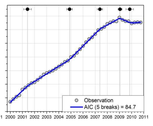
As we adjusted all sales prices to 2010 values utilizing the FHFA housing price index for Houston–
The Woodlands-Sugar Land, TX MSA, we utilize this index to identify the fixed effect time
segmentations in our data (δt). Specifically we apply a segmented regression methodology to the
quarterly Houston–The Woodlands-Sugar Land FHFA HPI values from 2001 to 2010 in order to
identify the unknown structural breakpoints in time for this housing market (Figure A.1, appendix).
Segmented or piecewise regression allows the detection of single or multiple change points at
unknown points in time (Muggeo, 2003). We detect five change points in the HPI data as
illustrated in the appendix: 1) 2001 between the 2nd and 3rd quarters; 2) 2004, between the 3rd
quarter and the 1st quarter of 2005; 3) 2007 between the 2nd and 3rd quarters; 4) 2009 between
the 1st and 2nd quarters; and 5) 2009 between the 3rd quarter and the 1st quarter of 2010. Given
these identified housing market breakpoints we account for their potential time effect in our
estimations by creating time interval dummy variables (δt) to represent each of them.10
Use of flood risk return periods (RP) in hedonic model
In order to account for the inherent variation in the flood risk within any designated flood zone we
ran separate regressions using the return periods. The specific discretized flood return periods
(RPs) that we use for our hedonic analysis are: RP ≤ 10; 10 < RP ≤ 25; 25 < RP ≤ 50; 50 < RP ≤
100; 100 < RP ≤ 250; 250 < RP ≤ 500; and RP > 500 (omitted category equating to X zone). We
ran three variations of models (1), (2), and (3) as explained above by replacing the FEMA
designated flood hazard zones with the RP dummy variables, i.e. a dummy equal to 1 if property i
14fall in RP ≤ 10 and 0 otherwise and so on. We note that according to the CoreLogic data there are
more than 13,000 properties within the Galveston County X zone that have a return period less
than 500 years when in theory zone X is the area determined to be outside the 500 year flood. This
discrepancy is probably due to FEMA flood hazard maps not always being completely in sync
with the actual flood return period (Czajkowski et al. 2013). However, for other zones (V /A
/X500) the return periods are comparable.
For the robustness of our above methods we perform two further analyses: 1) we examine
the possibility of subjective bias in our estimates using a Difference-in-Difference (DD) model
related to the occurrence of Hurricane Ike that made landfall in Galveston in September 2008 as
category 2 hurricane ; and 2) we estimate spatial hedonic models to account for the possible spatial
dependence among the neighboring properties.
A Difference-in-Difference (DD) Model to account for the impact of Hurricane Ike
The other main complication in the hedonic pricing of flood risk is that subjective bias of the
objective flood risk may exist in the community and thus flood risk will be not be a significant
attribute of housing prices (Chivers and Flores, 2002; Daniel et al., 2009; Bin and Landry 2012).
Often this bias is enhanced (reduced) by the occurrence (non-occurrence) of a significant flood
event (Kousky, 2010; Bin and Landry, 2012; Atreya et al. 2013). To examine the impact of
Hurricane Ike, if any, which made landfall in Galveston in September 2008 and caused extensive
flooding damage in Galveston County we estimate; i) a Difference-in-Difference (DD) model; and
ii) a separate model for only those home sales pre-Ike from 2001 to 2008. A DD design allows
us to isolate the effect attributable to flood from other contemporaneous variables since the control
group -which in or case will be the properties in the low flood risk zone/high return periods - will
15experience most of the contemporaneous impacts but offer lower flood risk. We use the following
specification for the DD model:
J K L N L
log( Pit ) o j S ijt k Likt l Ril m ln(C ) i n (ln(C ) i * Ril )
j 1 k 1 l 1 n 1 l 1
P L
(4)
ike p (ike * Ril ) i t it
p 1 l 1
where, variable ike is equal to 1 if the property was sold after Hurricane Ike made landfall (2009
onward) and 0 otherwise. In the above model the interaction coefficient between the variable Ike
and the risk variables (βp ) show how Hurricane Ike might have affected the prices of the properties
that are in the risk zones. For the flood risk variables we use both the FEMA flood zones and the
more granular return periods.
Spatial Hedonic Model accounting for the spatial dependence in the property prices
One of the econometric concerns in using a hedonic model is the presence of spatial dependence
among neighboring properties. Spatial dependence in property values can arise due to neighboring
properties sharing common features such as similar location amenities, similar structural attributes
due to common timing of construction. Recent critiques by McMillen (2010), Pinske and Slade
(2010) and Gibbons and Overman (2012) suggest that spatial models do not provide a valid
approach to causal identification, however, it is also argued that the use of spatial hedonic models
is appropriate since ignoring the spatial dependence in a hedonic analysis lead to an inefficient or
even inconsistent estimates. Therefore, to check for the robustness of our results we utilize the
spatial hedonic model allowing for spatial interactions in the dependent variable and the
disturbances.
16More formally, a spatial autoregressive model with autoregressive disturbance (SARAR)
is employed following Anselin and Bera, (1988) and Kelejian and Prucha (2010). The SARAR
model corresponding to model (3) above can be written as:
J K L
log( Pit ) o W ln( Pjt ) j S ijt k Likt l Ril m ln(C ) i
j 1 k 1 l 1
(5)
N L
n (ln(C ) i * Ril ) i t it
n 1 l 1
Where,
it M jt it ; it is i.id (assumed to be independent and identically distributed)
The spatial weights matrix W and M (W=M) are taken to be known and stochastic. The lambda
(λ) and rho (ρ) are the spatial lag parameter and spatial autocorrelation coefficient respectively.
Again we use both FEMA flood zone and return periods for the flood risk variables.
In spatial models, one of the challenges lies in defining an exogenous weights matrix (W)
that captures the relationship between the spatial units. In general, there is no consensus on
appropriate spatial weights matrix (Anselin and Bera, 1998). Queen Contiguity matrix and inverse
distance matrix are the most commonly used matrices in spatial models. Queen Contiguity matrix
is structured so that if the ith and jth properties share a common border or vertex, the elements of
the spatial weights matrix Wij receive a value of 1, 0 otherwise. The inverse distance matrix is
structured in such a way that the elements of the spatial weights matrix Wij receive a value equal
to inverse of Euclidian distance between the ith and jth properties. In our case we use a hybrid
matrix combining the queen contiguity and inverse distance matrix where distance decay was
allowed in the queen contiguity matrix. The hybrid matrix was min-max normalized.11 We employ
a generalized spatial two-stage least square (GS2SLS) estimator.12
17IV. Main Results
Table II presents the results of standard hedonic model that uses the FEMA flood zone
classifications of V, A, and X500 zones with the low risk X zone as the control group. We estimate
three different models as discussed in the methods section where model (1) includes the log of
coastal distance; in model (2), we control for distance to coast using coastal distance dummies
with 500 to 1000 feet increments for distance within a mile; and in model (3), we interacted the
flood zones with the log of coastal distance.
Across all three models, we find that the properties located in high-risk areas such as V and
A zones command a price premium (statistically significant at the 1 percent level in all three
models) suggesting that the associated positive amenity values of living in the 100 year flood zone
(V and A zone) in Galveston county outweigh the negative flood risk. This result is similar to
other coastal community estimates as shown by Bin and Kruse (2006) and Daniel et al. (2009),
where the positive amenity impacts of a coastal community has a strong effect. 13 The price
premium for V zone properties is 40.9 percent and 40.1 percent in model (1) and (2) respectively14
which means that a property in V zone sells for $74,311 and $72,676 more than an equivalent
property in the X zone (the control group) when evaluated at an average priced home ($181,690).
Likewise for the A zone, the price premium is equivalent to 8.12% and 9.6% in model (1) and (2)
respectively which means that a property in A zone sells for $14,739 and $17,309 than an
equivalent property in the X zone when evaluated at an average priced home ($181,690).
The variable ln_coast is negative and statistically significant in model (1), implying that
proximity to coast is highly desirable and increasing distance from the coast has strong negative
impact on the property prices.15 To put this in perspective, for an average priced home ($181,690),
moving away from the coastline 25,694 feet (average distance) results in a decrease in property
18values by $12,718 (7%). In model (2), we find that there is a monotonic decline in coastal
premium, from a 36% premium for properties located within 500 feet, to 12% for those between
500 feet and 1000 feet, to 7.6% for those between 1000 and 2000 going down to 3.9% for those
between 4000 and 5000 feet.
Using the model (1) coefficient results, Figure 5 illustrates the decay in the hedonic price
flood zone premium given increasing distance. For each (natural log) foot decreased from the
nearest coastline, sales prices decline by the same amount for all flood zones, 7 percent. Given
this equivalent distance decay rate for all flood zones, the V zone estimated hedonic premium
disappears after approximately 100 feet from the nearest coastline, whereas for the A zone it
disappears at approximately 10 feet.
To test the conditional impact of distance to coast and flood risk zones, in model (3) we
interact the negative amenity flood zone risk variable with the proximity to coast to estimate these
two variables acting together jointly on housing prices. We find a marked increase in the price
premium for the V zone properties of almost 146%, which is equivalent to $266,537 when
evaluated at an average priced home (Figure 6).16 However, note that this high premium is for the
properties in the V zone that are right on the coast and the premium decays as the distance from
the coast increases as suggested by negative and statistically significant coastdxVzone interaction.
For example, the premium decreases to almost 72.09 percent from 146 percent in V zone as the
distance from the coast increases to 100 feet which is equivalent to a decrease of $130,989 when
calculated for average priced home. 17 Similarly, compared to X zone properties the A zone
properties also command a marked price premium of 28% for the A zone properties that are right
on the coast which is equivalent to almost $52,000 when evaluated at an average priced home. We
19also find that the premium decays (negative and statistically significant coastdxAzone interaction)
as the distance to coast increases for A zone properties.
The interaction results illustrate the importance of accounting for these values acting jointly
on housing prices. While model (1) showed that the average rate of distance decay for all the zones
is constant at 7 percent, which is clearly not the case as demonstrated by model (3). The marginal
rate of distance decay for V zone property is 7.8 percent and the for A zone properties it is 1.8
percent. 18 That is, as the positive amenity value decreases with increasing distance from the
nearest coast, the remaining designated high flood risk is discounted more severely. Model (3)
results also indicate a negative price premium for X500 zone properties which is the opposite result
from the previous positive coefficients in models (1) and (2), although not statistically significant
at any meaningful level. We ran a likelihood ratio test to see if model (3) fitted the data better than
model (1). We find a χ2 value of 54.69 with a significant p-value suggesting that the difference
between the two models is significant and model (3) fits the data significantly better than model
(1).
Figure 6 shows the distance decay in the premiums as calculated using coefficients from
model (3) and thus accounting for the varying distance-amenity trade-offs by flood risk. In
comparison to Figure 5 (not accounting for this variation) we see now that hedonic premiums for
the V zone while decaying faster actually remain positive for nearly a quarter of a mile from the
nearest coastline. This impacts approximately 745 properties in the V zone with an estimated price
premium, whereas in model (1) this information was confounded and showed that the premium
existed for 44 properties within 100 feet of the nearest coastline. We see a similar result for the A
zone where in model (1) the hedonic price premium decayed away by 10 feet, has now expanded
to 100 feet impacting an additional 60 homes.
20Regarding the structural variables, across all three models in Table II the coefficient are
significant at one percent level and have expected signs except for variable stories which is
insignificant. As per the location variables, coefficient estimates indicate that being farther from
a bus route or park decreases property prices, whereas being nearby a school or railroad increases
property prices. The median household income have an expected positive sign. The NFIP dummy
is positive and significant suggesting that the properties that are built after the communities joined
NFIP in Galveston County are worth more, ceteris paribus. Also, the properties that are protected
by seawall are priced higher as suggested by positive and significant seawall dummy (Seawall),
likely due to the sense of safety that the seawall provides in the risky zones. In all the models, we
have included the time segment and the zip code fixed effects.
Accounting for varying flood risk return periods
To capture the effect of the inherent varying flood risk within any flood zone we replaced the
FEMA designated flood risk zones with the more granular return periods (RP) in our hedonic
estimations and estimated model (1), model (2) and model (3) with RP > 500 years as the omitted
categories. Table III presents these regression results.
From models (1) and (2) we see hedonic price premiums that are statistically significant up
to the 100 year RP and thus comparable to the V and A zone results in Table II. From model (3),
however, we see negative coefficient signs for all return periods greater than ten years with
statistical significance for RPs 25 to 50 and beyond 100 years, the X500 zone. Now, the only flood
risk area with a positive hedonic price premium from model (3) is the RPHowever, the hedonic price premium for RP
A Difference-in-Difference (DD) Model accounting for the impact of hurricane Ike

Table IV and V report the results from the DD models using aggregate flood zones as well as the

return periods respectively where column 1 in both tables gives the results of the DD model as in

equation (4), and column 2 gives the result of a hedonic model as in equation (3) using only the

pre-Ike sales data (2001-2008).19 From Table IV we find that there was no significant impact on

the property prices in the V zone due to the occurrence of Hurricane Ike as suggested by an

insignificant coefficient in the (Ike*V zone) interaction term. However, the statistically significant

(Ike*A zone) and (Ike*X500 zone) interaction terms indicate that property prices in A zone and

X500 zone decreased after Ike made landfall. V and A zone premiums in the DD model are also

lower in comparison to those from the 2001 to 2008 model. Importantly, in both columns statistical

significance and coefficient values/negative signs on the log of coastal distance and the flood zone

and distance interaction terms are comparable to the Table II results.

       From Table V we also find that there was no significant impact on the property prices in

the RP
the return periods respectively. Consistent with the results in Table II that uses the aggregate flood
zones, Table VI presents a positive and significant premium associated with the V zone and A
zone properties when also accounting for the spatial dependence. We also find that the premium
decays as the distance from the coast increases as suggested by negative and significant coefficient
of the distance and flood zone interaction term (coastxVzone & coastxAzone). All the other
variables such as structural attributes, location attributes, additional dummies (NFIP and Seawall),
time fixed effects and zip code fixed effects are included in all the models20 Regarding the spatial
parameters, we find that the spatial lag parameter (λ) is not significant suggesting that there is no
significant adjacency effect however, there is presence of spatial autocorrelation as suggested by
a significant spatial error parameter (ρ).
In table VII, we present results using the return periods instead of the aggregate flood zones
(comparable to table III results). Consistent with table III results, we find a significant premium
associated to the properties located in return period less than 10 years, the most risky zone.
However, after controlling for the distance to the coast conditional upon the risk return period in
model (3), we see negative and insignificant price premium for RP between 10 and 250 while
negative and significant premium for properties located in return period greater 250 and less than
500. In addition to these reported robustness tests we ran a series of other analyses not reported
here including: 1) separate spatial models for each aggregate flood zone (V zone and A zone) 2)
spatial hedonic model in DD framework for V and A zone separately 3) spatial hedonic model
using different spatial weighting matrices 4) separate models for mainland and island properties
and 5) models using the yearly time dummies. We were able to further verify the robustness of our
main results in each of the above cases.
24VI. Conclusions
We have attempted to estimate the effect on housing prices of locating near the coast through a
hedonic property analysis in Galveston County, TX allowing for the flood risk and coastal amenity
of living close to the water to act jointly on housing sales prices. We estimate these effects not
only through the traditional use of flood zones as a measure of the flood risk, but also incorporate
a more comprehensive measure of graduated flood risk through identified flood return periods.
Our results show that properties located in the high risk flood areas command a price premium
compared to those located outside. For example, the properties located in high-risk areas such as
V and A zones command a price premium of up to 146%. But this hedonic price premium is
dependent upon the distance to the coast, and as expected the distance effect varies by flood risk
type with found premiums to higher risk homes decaying at a faster rate the further one moves
away from the water. This illustrates the importance of capturing these two variables acting
together on sales prices. These results are also robust to the potential subjective bias associated
with the occurrence of Hurricane Ike in 2008.
Given the varying flood risk and distance tradeoffs captured in the interaction terms, we
show that properties located in the highest risk flood areas, for up to nearly a quarter mile from the
nearest coastline, command a sales price premium. These results directly contrast to some of the
previous hedonic property analyses findings that homes at the highest flood risk will sell at a
discount to account for higher flood insurance rates being capitalized into housing sales prices. We
acknowledge that our measure of positive water amenities – distance to the nearest coast – may
not fully represent the variety of positive amenities inherent to living near the water. Thus, we
additionally controlled for the impact of other possible coastal amenities such as including
waterfront properties (dummy=1 if property is within 500ft from the coast) as well as adding
25distance to the nearest beach access points in our models. In both cases, we still find a premium
associated with V and A zone properties, although of a lower magnitude, with the coefficient on
distance to beach access points being relatively small in magnitude and statistically insignificant
at the 10 percent level.21While another coastal amenity of interest could be the measure of view,
Daniel et al. (2009) find that distance is a more meaningful control for positive water amenities
than view. Other measures of positive water amenities warrant more attention in future flood risk
and housing price research.
Therefore, the assertion by realtors, homebuilders, and lenders in opposition to BW-12 that
moving to risk-based premiums will cause property values to steeply decline and make homes
unsellable is not universally true in our study area. We show that this depressed property value
assertion is sensitive to the distance to water. The powerful amenity value provided by the nearby
coastal water shadows the flood risk and therefore masks the influence of increased flood insurance
premiums on property prices. Notably, even with our systematic interaction approach coupled
with more detailed flood risk return period data, we find that in the absence of a major flood event
it is difficult for the negative flood amenity value based upon the objective flood risk to sufficiently
counteract a homeowner’s strong desire to live near the water.
26References:
Arraiz, I., Drukker, D. M., Kelejian, H.H., and Prucha I. R. 2010. “A Spatial Cliff-Ord Type
Model with Heteroskedastic Innovations: Small and Large Sample Results.” Journal of Regional
Science 50 (2): 592–614.
Anselin, L., and Bera A.1998. “Spatial Dependence in Linear Regression Models with an
Introduction to Spatial Econometrics.” In Handbook of Applied Economic Statistics, eds A.
Ullah and D. Giles.
Atreya, A., Ferreira, S., and Kriesel, W.P. 2013. “Forgetting the Flood? An analysis of the Flood
Risk Discount over Time.” Land Economics 89 (4): 577-596
Barnard, J.R., 1978. Externalities from urban growth: the case of increased storm runoff
Bin, O., and Polasky, S. 2004. “Effects of Flood Hazards on Property Values: Evidence before
and after Hurricane Floyd.” Land Economics 80 (4): 490–500.
Bin, O., and Kruse, J.B. 2006. “Real Estate Market Response to Coastal Flood Hazards.” Natural
Hazards Review 7 (4): 137–44.
Bin, O., Kruse, J. B, and Landry, C. E. 2008a. “Flood Hazards, Insurance Rates, and Amenities:
Evidence from the Coastal Housing Market.” Journal of Risk and Insurance 75 (1): 63–82.
Bin O., Crawford, T. W., Kruse, J. B., and Landry, C. E. 2008b. Viewscapes and flood hazard:
Coastal housing market response to amenities and risk. Land Economics 84(3): 434–48
Bin, O., and Landry, C. E. 2012. “Changes in Implicit Flood Risk Premiums: Empirical
Evidence from the Housing Market.” Journal of Environmental Economics and Management 65
(3): 361–76.
Boyle, K., Lewis L., Pope J., and Zabel. 2012. “Valuation in a bubble: Hedonic modeling pre and
post-housing market collapse.” AERE Newsletter, 32(2).
Conroy, S. J., & Milosch, J. L. 2011. “An estimation of the coastal premium for residential
housing prices in San Diego County.” The Journal of Real Estate Finance and Economics, 42(2),
211-228.
Czajkowski, J., Kunreuther, H., & Michel‐Kerjan, E. 2013. “Quantifying Riverine and Storm‐
Surge Flood Risk by Single‐Family Residence: Application to Texas.” Risk Analysis
33(12):2092-2110
Chivers, J. and Flores, N. E. 2002. “Market Failure Information: The National Flood Insurance
Program”. Land Economics, 78(4):515-521
27Daniel, V., Florax, R., Rietveld, P., 2009. Flooding Risk and Housing Values: An Economic
Assessment of Environmental Hazard. Ecological Economics 69(2):355-365
Drukker, D. M., Egger, P. and Prucha, I. R. 2009. On Single Equation GMM Estimation of a
Spatial Autoregressive Model with Spatially Autoregressive Disturbance. Technical report,
Department of Economics, University of Maryland.
FEMA 2014. http://www.fema.gov/national-flood-insurance-program/base-flood-elevation
FEMA 2014. http://www.fema.gov/policy-claim-statistics-flood-insurance/policy-claim-
statistics-flood-insurance/policy-claim-13
FHFA 2014, http://research.stlouisfed.org/fred2/series/ATNHPIUS26420Q
Freeman, A. 2003. The measurement of environmental and resource values: theory and methods:
RFF press.
Gibbons, S. and Overman, H. G.. 2012. “Mostly Pointless Spatial Econometrics?” Journal of
RegionalScience 52(2):172 – 191
Griffith, R. S.1994. The Impact of Mandatory Purchase Requirements for Flood Insurance on
Real Estate Markets, Doctoral Dissertation, University of Texas at Arlington, August.
Insurance Journal, 2014. House Passes Flood Insurance Bill; Key Senators Sign On Available
at http://www.insurancejournal.com/news/national/2014/03/04/322194.htm
Kelejian, H.H., and Prucha, I.R. 2010. "Specification and estimation of spatial autoregressive
models with autoregressive and heteroskedastic disturbances." Journal of Econometrics
157(1):53-67.
Kousky, C. 2010. “Learning from Extreme Events: Risk Perceptions after the Flood.” Land
Economics 86 (3): 395–422.
Kriesel, W., Friedman, R. 2002. Coastal hazards and economic externality: implications for
beach management policies in the American South East. H. John Heinz III Center for Science,
Economics and the Environment, Washington DC.
McKenzie, R., Levendis, J. 2010. Flood Hazards and Urban Housing Markets: The Effects of
Katrina on New Orleans. Journal of Real Estate Finance and Economics 40:1:62-76
McMillen, Daniel P. 2010. “Issues in Spatial Data Analysis,” Journal of Regional Science, 50(1):
119–141.
Michel-Kerjan, E., Czajkowski, J., Kunreuther, H. 2014. Could Flood Insurance Be Privatized in
the United States? A Primer, The Geneva Papers, forthcoming.
28Morgan, A. 2007. The impact of Hurricane Ivan on expected flood losses, perceived flood risk,
and property values. Journal of housing research, 16(1), 47-60.
Muggeo, V.M.R., 2003. “Estimating regression models with unknown break-points” Statistics in
Medicine, 22: 3055-3071.
Pinske, J. and Slade, M.E. 2010. “The Future of Spatial Econometrics,” Journal of Regional
Science, 50(1), 103–117.
Posey, J., & Rogers, W. H. 2010. The impact of Special flood Hazard Area designation on
residential property values. Public Works management & Policy, 15(2), 81-90.
Rosen, S. 1974. “Hedonic Prices and Implicit Markets: Product Differentiation in Pure
Competition,” Journal of Political Economy 82(1): 34-55.
Tobin, G.A., Montz, B.E., 1994. The flood hazard and dynamics of the urban residential land
market. Water Resources Bulletin 30 (4), 673–685.
US Army Corps of Engineers (USACE), 1998. Empirical studies of the effect of flood risk on
housing prices. Alexandria, Virginia, Water Resources Support Center Institute for
Water Resources.
Wall Street Journal (WSJ) 2013. Flood Program Puts Industries at Odds.
http://online.wsj.com/news/articles/SB10001424052702304773104579268620558111400
Zhai, G., Fukuzono, T., Ikeda, S., 2003. Effect of flooding on megalopolitan land prices: a case
study of the 2000 Tokai flood in Japan. Journal of Natural Disaster Science 25 (1), 23–36.
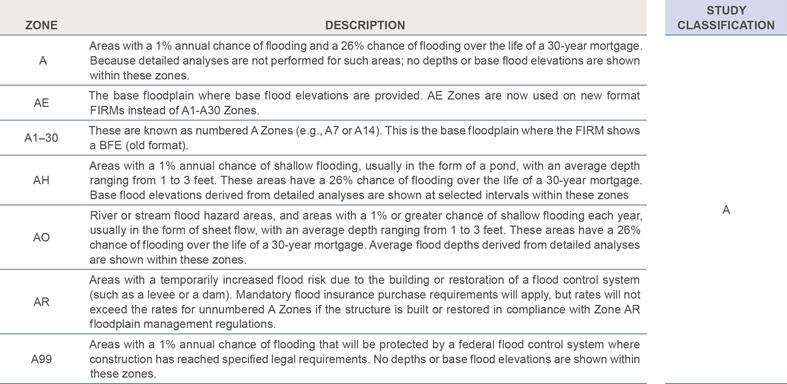
29APPENDIX: Definitions of FEMA Flood Zone Designations
Flood zones are geographic areas that the FEMA has defined according to varying levels of flood risk. These zones are depicted on
a community's Flood Insurance Rate Map (FIRM) or Flood Hazard Boundary Map. Each zone reflects the severity or type of flooding
in the area.
Moderate to Low Risk Areas
In communities that participate in the NFIP, flood insurance is available to all property owners and renters in these zones:
High Risk Areas
In communities that participate in the NFIP, mandatory flood insurance purchase requirements apply to all of these zones:
High Risk - Coastal Areas
In communities that participate in the NFIP, mandatory flood insurance purchase requirements apply to all of these zones:
30You can also read