Accurately predicting electron beam deflections in fringing fields of a solenoid - Nature
←
→
Page content transcription
If your browser does not render page correctly, please read the page content below
www.nature.com/scientificreports
OPEN Accurately predicting electron
beam deflections in fringing fields
of a solenoid
Christof Baumgärtel, Ray T. Smith & Simon Maher*
Computer modelling is widely used in the design of scientific instrumentation for manipulating
charged particles, for instance: to evaluate the behaviour of proposed designs, to determine the
effects of manufacturing imperfections and to optimise the performance of apparatus. For solenoids,
to predict charged particle trajectories, accurate values for the magnetic field through which charged
species traverse are required, particularly at the end regions where fringe fields are most prevalent. In
this paper, we describe a model that accurately predicts the deflection of an electron beam trajectory
in the vicinity of the fringing field of a solenoid. The approach produces accurate beam deflection
predictions in the fringe field region as well as in the centre of the solenoid. The model is based on a
direct-line-of-action force between charges and is compared against field-based approaches including
a commercially available package, with experimental verification (for three distinct cases). The direct-
action model is shown to be more accurate than the other models relative to the experimental results
obtained.
Charged particle dynamics (also known as charged particle optics) is concerned with the manipulation of charged
particles (e.g., electrons, protons, ions) within an electric and/or magnetic field. The deflection of charged parti-
cles by electromagnetic fields has widespread and important connotations in physical sciences, engineering, life
sciences and for a wide range of technologies. An understanding of the electrical forces at play between charges is
essential and has long been applied to a multitude of high-tech applications, from particle accelerators1–4, deceler-
ators (e.g., storage rings)5,6, electron microscopes7,8, electronics 9, nuclear fusion reactors10,11 and magnetrons12,13,
through to medical diagnostics (e.g., radiation therapy)14,15, mass s pectrometry16 and electron beam w elding17,18,
amongst many others.
The simulation and prediction of beam trajectories is of great importance for design purposes, especially
for low energy beams where perturbing effects such as space charge and fringe fields are prevalent in the low
velocity regime and can impede the accuracy of predictions. In particular, fringe fields are known to introduce
non-linearities that induce a variety of undesired effects, such as influencing particle motion by sudden shifts in
position, as well as tune shifts and chromaticity s hifts19 leading to beam instability. When developing new instru-
mentation for manipulating charged species, both the cost and practicality of assembly make it extremely difficult
and time-consuming to test (experimentally) the behaviour of different designs. Hence, it is common for many
of the application areas already noted to utilise accurate simulation of performance prior to construction. This is
an important step when designing charged particle apparatus and particularly for more advanced systems, such
as unconventional and/or high performance setups, as it is vital in securing cost-effectiveness and functionality.
Solutions for electromagnetic problems, including those encountered in the field of charged particle optics,
are often solved numerically using the finite element (FE)20, finite difference (FD)21 or boundary element (BE)
methods22. These methods have been hugely successful and each has its own benefits and drawbacks broadly
relating to accuracy, resolution, computational time and memory r equirements23, yet fundamentally they are all
solving the same equation set based on Maxwell–Lorentz.
In this paper we present a novel model for charged particle deflection in the low velocity regime, v ≪ c , which
is formed from a fundamentally different approach as compared to the field theory approach of Maxwell–Lorentz.
According to field theory, a particle’s deflection is governed by the Lorentz force equation,
Department of Electrical Engineering and Electronics, University of Liverpool, Liverpool, UK. *email: s.maher@
liverpool.ac.uk
Scientific Reports | (2020) 10:10903 | https://doi.org/10.1038/s41598-020-67596-0 1
Vol.:(0123456789)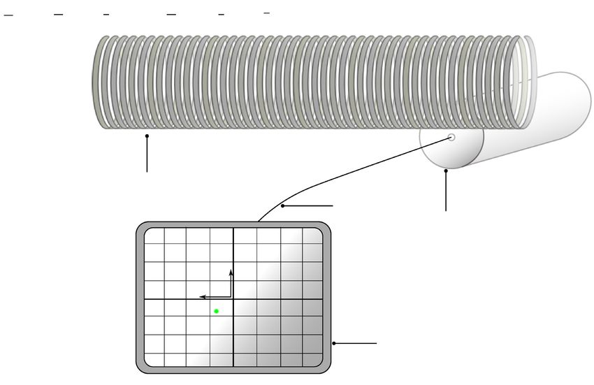
www.nature.com/scientificreports/
F� = q(E� + v� × B
� ), (1)
that relates the deflection of a charge, q, moving at speed, v , to the electrical field strength, E , and the magnetic
field strength, B
. By contrast, the new model proposed herein, is based on a direct physical approach involving
a direct-line-of-action force between charges in the low velocity regime. Specifically, we are concerned with the
interaction between the charge carriers in an electron beam and those within a current carrying solenoid, which
forms the basis of an investigation to predict the behaviour of a charged particle beam in the region of a fringing
magnetic field. The solenoid is key in this regard, as it has long been established as a fundamental charge optical
element for generating a controlled magnetic field that is widely used for manipulating charged particles (e.g.,
focusing and beam guiding). Moreover, it is well-known that the motion of charged particles in the vicinity of
a solenoid, particularly near the entrance and exit, are subject to non-linear effects that can have a significant
impact on particle trajectories that are difficult to accurately p redict24–27.
Our model is compared with the predictions of field-theory, including state-of-the-art commercially avail-
able software22 as well as calculations by Cébron28 which are based on the work of Callaghan and Maslen29 and
Derby and O lbert30. These field calculations form the basis of further work on finite solenoids with a permeable
core , internal magnetic fields of off-axis solenoids32 and parallel finite solenoids33, even to the application of
31
axis alignment measurements of s olenoids34–36.
To evaluate the validity and accuracy of both model types (field versus direct-line-of-action force), an experi-
ment is set up that employs a modified electron gun whose beam is made to pass across a variety of current car-
rying solenoids from whence the beam is deflected. By locating the solenoids at different positions with respect
to the electron gun, it is then possible to investigate the deflection caused by significant fringing fields which are
associated with short solenoids and the end regions of a given solenoid.
Mathematical model
Three different models which predict the deflection of an electron beam passing across a solenoid in any field
region are presented and explained in this section: (i) the standard (i.e., conventional) model following the field-
based approach of electrodynamics (Sect. ‘Field model’) where the interaction of all charged particles is based
on the Maxwellian theory of electric and magnetic fi elds28–30; (ii) a numerical model based on field theory (Sect.
‘Modelling with CPO’) from the software package C PO22, which is used to calculate beam trajectories based
on the Boundary-Element-Method (BEM); (iii) our model (Sect. ‘Weber model’) which employs the theory of
direct action at a distance between the particles and is based on Weber electrodynamics, where the concept of
field entities E & B and their mediation is avoided. In this paper, we develop a new model based on the Weber
force equation to predict the trajectory of an electron beam and its deflection accordingly. Recently, there has
been increased research interest in Weber-based electrodynamics, where the theory has been related not only to
electron beam d eflection37,38, but also to i nduction39,40, superconductivity41,42 as well as the Planck-constant43,44
and the structure of the atom45,46. First, the Weber-based model will be explained in the following section.
Weber model. The model we present follows the direct action approach laid out by W eber47, where he pub-
lished his findings 15 years prior to Maxwell’s t heory48 of fields and aether. The interaction of charged particles
according to Weber is determined by the Weber-force equation,
q1 q2 r̂12
2
ṙ12 r12 r̈12
�
F21 = 1− 2 + (2)
4πε0 r12 2 2c c2
that depends on the relative displacement r 12, relative velocity r12
˙ and relative acceleration r12
¨ between the charges
q1 and q2, where ε0 is the permittivity of free space and c is the speed of light. In this formulation we have
�r12 =�r1 − �r2 (3)
dr12
ṙ12 = = r̂12 · v�12 (4)
dt
d 2 r12 dṙ12 [�v12 · v�12 − (r̂12 · v�12 )2 + �r12 · a�12 ]
r̈12 = = = (5)
dt 2 dt r12
along with the magnitude and unit vector in equation (6).
�r12
r12 = |�r1 − �r2 | r̂12 = (6)
r12
The Weber force acts along the line joining the particles and reduces to the Coulomb force for charges at rest.
axwell49–52, although it does not depend on them conceptually,
It is also consistent with the field equations of M
as it is a direct-action approach where a form of mediation is not needed to transmit the force between charges.
Based on this force approach a model has been derived in an earlier w ork37 for the deflection of electrons across
a single current loop, but to apply this to the fringing field regions, significant refinements have been added to
the simplified two dimensional (2D) model o f37, especially to account for the three dimensional (3D) nature,
taking the geometry of the particular solenoid into account. As a first step, however, a single current loop can
Scientific Reports | (2020) 10:10903 | https://doi.org/10.1038/s41598-020-67596-0 2
Vol:.(1234567890)www.nature.com/scientificreports/
electron beam v1
r12 Electron Beam
v2 z3
y +dzθ
I dθ z1
y r2 r1 h
z Ri R
o
θ x
x
R −dzθ Solenoid
z2
l −l
2 2
(a) (b)
Figure 1. Geometry and system of coordinates to model the electron beam and solenoid: a Simplified 2D
geometry for a single current carrying loop and an electron beam travelling parallel to the x-axis; b Expanded
3D geometry with the coordinate origin at the centre of the double wound solenoid with the beam at a position,
z1, travelling parallel to the x-axis.
be assumed in a 2D plane, where the electron beam is traversing across the solenoid at a fixed height, h, in the
positive x-direction with a velocity, v 1, giving it a position, r1, as shown in Fig. 1a.
The current, I, is situated at a position, r2, and rotating here in a positive mathematical sense, with a velocity,
v 2, around the loop with a radius, R, so that it can be represented by a current element, IRdθ . It is important
to note that the rotational direction of the current is regarded as the actual physical motion undertaken by the
electrons in the current element, so it is in opposition to the conventional current flow, and rather sticks to the
physical direction of current flow.
As a next step the model is now extended to 3D space, with the coordinate system being centred in the
solenoid, with the solenoid axis elongating from − 2l to 2l . For the experiments, the solenoids used are all double
wound with a given number of windings, and to take the double wound manufacturing into account in the
model, the force is split into an inner and outer component, Fi and Fo, respectively, with a coil radius of Ri and
Ro which are about the same, Ri ≈ Ro. We assume that the electron-current is fed to the solenoid at the position
z2 = 2l to one layer of the winding, so that it moves towards z3 = − 2l and is then returning through the other
layer towards z2, as depicted in Fig. 1b.
This behaviour can be modelled in two ways, one is a helical motion following the pitch of the windings and
the other one is a summation model, where each winding is assumed as a single current loop at a given position
and the principle of superposition is used to summate the force contribution from each individual loop. For
the helical model the current is then changing its axial position, depending on the pitch with dz · θ , either in a
positive or negative sense, depending on where the current is fed and returned to. The corresponding velocity
increase along the axis is derived as vR2 dz and the relational position, r12, and velocity, v 12, are defined as:
x1 R cos(θ) R cos(θ)
�r1 = h �r2i = R sin(θ) �r2o = R sin(θ) (7)
z1 z2 − dzθ z3 + dzθ
x1 − R cos(θ) x1 − R cos(θ)
�r12i = h − R sin(θ) �r12o = h − R sin(θ) (8)
z1 − z2 + dzθ z1 − z3 − dzθ
(9)
r12i = (x1 − R cos(θ))2 + (h − R sin(θ))2 + (z1 − z2 + dzθ )2
(10)
r12o = (x1 − R cos(θ))2 + (h − R sin(θ))2 + (z1 − z3 − dzθ)2
v1 −v2 sin(θ) −v2 sin(θ) v1 + v2 sin(θ)
� �
v�1 = 0 v�2i = v2 cos(θ) v�2o = v2 cos(θ) v�12i,o = −v2 cos(θ) (11)
0 − vR2 dz v2
R dz ± vR2 dz
It is further assumed that the acceleration is negligible for the given experimental setup, as the electrons in the
beam are moving at a constant speed after the initial acceleration phase and the acceleration that is exerted on
the current element due to the helical motion is sufficiently small.
In order to calculate the resulting force between the beam and the current in the solenoid a superposition
of all the charges involved must be performed. Physically, the electrons in the beam are interacting with the
Scientific Reports | (2020) 10:10903 | https://doi.org/10.1038/s41598-020-67596-0 3
Vol.:(0123456789)www.nature.com/scientificreports/
electrons in the current element and also the positive charges in the static metallic lattice of the solenoid. With
q1− = −q1+ and q2− = −q2+, as well as v1 ≫ v2, we get:
F�ihelix = F�i1−2− + F�i1−2+
q1+ q2+ v1 v2 �r12i (x − R cos θ)2 (x − R cos θ)(h − R sin θ)
= 2 sin θ − 3 sin θ + 3 cos θ
2
4πε0 c r12i 3 2
r12i 2
r12i (12)
dz (x − R cos θ)(z1 − z2 + dzθ )
−3 2
R r12i
F�ohelix = F�o1−2− + F�o1−2+
q1+ q2+ v1 v2 �r12o (x − R cos θ)2 (x − R cos θ)(h − R sin θ)
= 2 sin θ − 3 sin θ + 3 cos θ
2
4πε0 c r12o 3 2
r12o 2
r12o (13)
dz (x − R cos θ)(z1 − z3 − dzθ )
+3 2
R r12o
For the summation model each single loop is assumed to be positioned at one distinct point on the solenoid axis
p · (n − 1), with p being the pitch of the winding and the integer index n = 1 . . . N , where N is the total number
of turns in one layer. Accordingly, the current element is only moving in the 2D plane at each loop, thus not
having an axial velocity component. The inner and outer forces are then found to be:
F�isummation = F�i1−2− + F�i1−2+
q1+ q2+ v1 v2 �r12i (x − R cos θ)2 (x − R cos θ)(h − R sin θ)
= 3
2 sin θ − 3 sin θ 2
+ 3 cos θ 2
4πε0 c 2 r12i r12i r12i
(14)
F�osummation = F�o1−2− + F�o1−2+
q1+ q2+ v1 v2 �r12o (x − R cos θ)2 (x − R cos θ)(h − R sin θ)
= 3
2 sin θ − 3 sin θ 2
+ 3 cos θ 2
4πε0 c 2 r12o r12o r12o
(15)
To evaluate the total force exerted by the solenoid on the beam, we can assume that while the continuous current
is flowing, a current element is immediately replaced with the next. The transformation qv → v → IRdθ then
holds the total force for integrating over the complete solenoid. This yields force equations for both Weber-based
models,
q1+ v1 I N·2π �r12i (x − R cos θ)2 (x − R cos θ)(h − R sin θ)
F�Whelix = 2 3
2 sin θ − 3 sin θ 2
+ 3 cos θ 2
4πε0 c 0 r12i r12i r12i
dz (x − R cos θ)(z1 − z2 + dzθ) �r12o (x − R cos θ )2
−3 2
+ 3
2 sin θ − 3 sin θ 2 (16)
R r12i r12o r12o
(x − R cos θ)(h − R sin θ) dz (x − R cos θ)(z1 − z3 − dzθ )
+ 3 cos θ 2
+3 2
Rdθ
r12o R r12o
N
q1+ v1 I 2π �r12i (x − R cos θ )2 (x − R cos θ)(h − R sin θ)
F�Wsum = 2 3
2 sin θ − 3 sin θ 2
+ 3 cos θ 2
4πε0 c r r r12i
n=1 0 12i 12i
�r12o (x − R cos θ)2 (x − R cos θ)(h − R sin θ)
+ 3 2 sin θ − 3 sin θ 2
+3 cos θ 2
Rdθ
r12o r12o r12o
(17)
where N is the number of turns in one layer. From both of these equations it is evident that the model predicts
three kinds of forces on the beam: a longitudinal force, a vertically transversal force and a horizontally trans-
versal force. The beam will then be deflected in the y-direction due to the transverse (vertical) force and in the
z-direction due to the (horizontal) transverse force. Therefore the impulse of the force is calculated with the time,
t, that the beam spends travelling from the anode to a fluorescent screen (that is excited upon electron collision)
on which the deflection is recorded.
t
�J = F�W dt (18)
0
Equating this to the change of vertical and horizontal momentum,
Jv = me vv , Jh = me vh (19)
Scientific Reports | (2020) 10:10903 | https://doi.org/10.1038/s41598-020-67596-0 4
Vol:.(1234567890)www.nature.com/scientificreports/
where me is the electron mass and vh , vv are the horizontal and vertical velocities gained from the deflection
force, the total deflections can be calculated as,
1 2 1 1 Jv 1 2 1 1 Jh
yd = av t = vv t = t, zd = ah t = vh t = t (20)
2 2 2 me 2 2 2 me
In order to accurately predict these deflections, they have been simulated in Matlab (Mathworks) with numerical
integration based on the trapezium rule to an accuracy of 0.1 mm for the spatial beam propagation and 0.5◦ for
the integration step size. The simulations show that the helical and summation approach both arrive at the same
force for the respective direction, which was anticipated, given the chosen modelling approach. It also serves
to verify the choices made to model the axial elongation of the solenoid. Further to this, the longitudinal force
acting along the beam is found to be zero, which is in agreement with the Lorentz-force vector. On the other
hand, the deflections occurring transversal to the beam are both expected due to the vector cross product v� × B �
in the Lorentz-formula, as will be seen clearly in the field-based model in the next section. From this model it
can also be deduced that the direction of deflection depends on the rotational direction of the current, which in
the standard field model determines the magnetic field direction and thus the corresponding deflection. Here
we can find a deflection of the beam in the positive y-direction and negative z-direction for mathematically
positive rotating electrons and in the case of negative rotation, the deflection occurs in negative y- and positive
z-direction. This is consistent for the expected vertical deflection direction from the right-hand-rule, respectively
left-hand-rule in the standard field based approach, which will be examined next.
Field model. For the calculation of the magnetic field a Matlab code by D. Cébron is used28 which is based
on the work of Derby and O lbert30 and Callaghan and M aslen29. The latter is contained in a technical note from
NASA, in order to calculate the fields inside and outside of any finite solenoid or magnet. This simulates the
radial component, Bρ , and the axial component, Bz , based on the residual field, Bres = µ0 nunit I , with nunit being
the number of turns per unit length, and then solving the complete elliptic integrals for the magnetic fields.
These are28:
2 −2
+
Bres R ω± E (ω± )
Bρ = K(ω± ) + (21)
π ρ 2ω± ω± −
where K and E are the complete elliptic integrals of the first and second kind and
4Rρ
ω± = (22)
(R + ρ)2 + ξ±2
with ξ± = z ± L/2. Then the following definitions are made for the axial magnetic field,
γ =(R − ρ)/(R + ρ), (23)
(R − ρ)2 + ξ±2
ζ± = , (24)
(R + ρ)2 + ξ±2
ξ±
χ± = .
(25)
(R + ρ)2 + ξ±2
The axial field is then for ζ+ < 1
+
Br R 1
Bz = χ± K 2 2
1 − ζ± + γ � 1 − γ , 1 − ζ± (26)
π R+ρ γ +1 −
and for ζ± 1
+
Br R 1 χ± 1 1 1
Bz = γK 1− 2 +� 1− 2, 1− 2 (27)
π R + ρ γ (γ + 1) ζ± ζ± γ ζ±
−
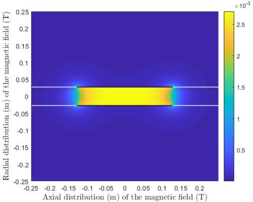
with being the complete elliptic integral of the third kind. The total calculated field strength with this approach
can be seen in Fig. 2 which has been simulated with the same accuracy as in the ‘Weber model’ section. The white
lines in the Figure, situated at ±R , are where the algorithm used did not converge.
Next, to perform the vector cross product and deduce the deflection along the y and z axes, we convert the
field to Cartesian coordinates at an angle of θ = 32 π as the beam passes below the solenoid. Thus
0
� = −Bρ
B (28)
Bz
and we can get the deflecting force
Scientific Reports | (2020) 10:10903 | https://doi.org/10.1038/s41598-020-67596-0 5
Vol.:(0123456789)www.nature.com/scientificreports/
Figure 2. Field of solenoid S2 generated with the field calculations from28. The field strength (T) is shown
around the solenoid, except for the white lines at the radial position ρ = R, as the algorithm did not converge at
these points.
� ).
F�L = q(�v1 × B (29)
me ve2
With that the Larmor radius can be obtained in the usual way, rL = FL and the deflection is obtained by using
rL ± rL2 − d 2 , where d is the travel distance of the beam and the sign depends on the direction of deflection.
Apart from that, an impulse approach was also used to calculate the deflections, where the force acting on
the beam has been calculated following the beam trajectory, starting from the position where the Larmor radius
is obtained to the point where the beam is intercepted by the fluorescent screen. Thus, the local force is obtained
with the same granularity as in the previously described model. The forces can then be integrated according to
Eq. (18) and the final deflection is again obtained using Eq. (20). Both Larmor radius and impulse approach then
give the same results for deflections in the y and z directions.
Additionally, the model by Farley and Price53 to roughly estimate the field of a finite solenoid has also been
used to check the deflection at the position z1 = 0 when the beam is centred across the coil. This model however,
can only predict the vertical deflection at that specific point as it was not designed for inhomogeneous fields.
Modelling with CPO. Finally, the deflections across the solenoid are also modelled with state-of-the-art
commercially available software CPO22. Here the solenoid is modelled as a stack of current loops, which is one of
the two standard methods available in the software. Following the geometries shown in the ‘Experimental setup’
section, the solenoid is set to elongate on the z-axis and with the coordinate origin aligning with the centre of the
solenoid. A current of 1.00 A is supplied to rotate in the mathematically negative sense, which represents positive
rotation of the electrons moving through the solenoid. The beam going across the solenoid is seen as individual
rays of electrons and traced with the direct method. Both the databuilder file that is used to implement the
experimental setup and the field that is generated by the software (see Fig. SF1) are given in the supplementary
information. The simulation results to model electron beam deflection across a solenoid from these three models
can be found in Tables 2 and 3 in the ‘Results’ section, where they are also compared to the experimental results.
Experimental setup
A sketch of the relatively simple experimental setup is shown in Fig. 3, depicting an electron beam (from an
electron gun) which is deflected across the current carrying solenoid and then strikes a fluorescent screen. The
electron gun and the fluorescent screen were adapted from a Hameg 203-6 cathode ray oscilloscope, so that
Scientific Reports | (2020) 10:10903 | https://doi.org/10.1038/s41598-020-67596-0 6
Vol:.(1234567890)www.nature.com/scientificreports/
3l 5l l 3l l l
0
4 8 2 8 4 8
Solenoid
Electron
Beam
Electron gun
y
z
Fluorescent Screen
Figure 3. Solenoid positioned across the electron beam from the electron gun at z1 = 0 where the electrons are
deflected and intercepted by the fluorescent screen with an indicated beam spot (green). Also depicted are the
positions 8l to 3l4 where the beam can also be positioned with reference to the centre of the solenoid.
Solenoid Radius (mm) Length (mm) Absolute number of windings and [nunit] Current (A)
S1 20 25 61 [2440] 1.00
S2 27 255 560 [2200] 1.00
S3 30 500 1300 [2600] 1.00
Table 1. Properties of the three Solenoids S1, S2 and S3 that are used in the experiments.
the solenoid can be located across the electron beam, at right angles to the electron beam. The circuitry of the
oscilloscope has been modified into a control unit that connects to the electron gun through an external cable.
The electron gun tube operates at an acceleration voltage of 2000V, which gives the electrons a terminal
velocity of
2eV
ve = ≈ 2.65 × 10⁷ m s−1 (30)
me
after passing the anode, at a distance of 7 cm from emission. Propagating in a straight line the fluorescent screen
is then intercepted after another 21.5 cm of beam travel. The glass evacuated tube enclosing the electron gun has
a diameter of 50 mm and the solenoid sits on top of it, at a distance of 3 cm from the anode. For our choice of
coordinates, the beam propagates at a height h = −(25 + R) mm and travels 18.5 cm from the coordinate origin
to the fluorescent screen with this arrangement.
The phosphor screen has a graticule divided in 10 mm steps, with subdivisions of 2 mm that give a rough
indication of where the beam is intercepted by the screen after the deflection. The spot left by the beam can be
focused to a size of roughly 1 mm in diameter and is indicated by the green coloured spot in Fig 3. To deflect the
beam, three different solenoids are used: length 25 mm (S1), length 255 mm (S2) and length 500 mm (S3), with
different radii and numbers of windings, as documented in Table 1. By definition, the shortest solenoid with 25
mm length can be considered as a ‘coil’, but will be further referred to as solenoid S1. A continuous DC-current
of 1.00 A is supplied to the solenoid with a benchtop power supply.
The solenoids are set in such a way that the beam is deflected at different positions relative to the coordinate
origin, so that the beam crosses different regions of the field, which are getting increasingly more fringing closer
to the solenoid ends. For the shortest solenoid, it is first set for the beam to cross at z1 = 0, per se at the middle
Scientific Reports | (2020) 10:10903 | https://doi.org/10.1038/s41598-020-67596-0 7
Vol.:(0123456789)www.nature.com/scientificreports/
11
10
9
8
7
6
5
4
3
2
1
-9 -8 -7 -6 -5 -4 -3 -2 -1 0
Figure 4. Measured and predicted deflections of the electron beam across S1 for both vertical and horizontal
directions. In the bubble chart, the blue squares show the experimental data and are labelled with the beam
position relative to the solenoid centre, i.e. the axial or “z”-position (as illustrated in Figure 3). For each given
beam position, the size of the data points relating to that position are uniquely the same size, so that predictions
from the Weber model (red x), Field model (yellow triangle) and CPO (purple circle) all have the same size
marker (as the corresponding blue square/experimental measurement) for each given “z” position.
of the solenoid length and then moved in steps of one quarter of the length towards the edge of the solenoid,
so that it passes at z1 = 4l and then at z1 = 2l where it is aligned with the end of the solenoid on the z-axis. The
solenoid is then moved for the beam to be positioned at z1 = 3l4 and z1 = l , while the solenoid is kept at the same
height. At these points the beam is not crossing the coil directly any more, as it sits at a distance further from the
origin than the solenoid’s axial elongation. These positions are also implied in Fig. 3 for a visual representation
of where the beam is travelling in relation to the solenoid origin.
For the two longer solenoids, S2 and S3, the beam is set in 18 steps of the solenoid length from the centre posi-
tion, z1 = 0, up to the point z1 = 3l4 which are again shown in Fig. 3. Especially at the positions around z1 = 2l , it
is said that the field is fringing and strongly deviates from the ideal homogeneous field associated with an infinite
solenoid. Furthermore, the shortest coil, S1, will have a very inhomogeneous field according to theory due to its
length and radius being almost the same, with a relatively small number of windings.
To obtain measurement of beam deflections the following procedure is adopted. The solenoid is located at
a given position across the e beam which is then focused and centred in the middle of the screen. The solenoid
current is now switched on and adjusted to provide a magnitude of 1.00 A; the beam deflection is noted. The
deflection on the screen is acquired with a plastic vernier along with the help of the graticule on the screen;
immediately after the power supply is switched off. The procedure is repeated 3 times in order to acquire a mean
deflection for the beam spot.
Results and discussion
The beam deflections measured in the vertical and horizontal directions across the three solenoids are summa-
rised in Figs. 4, 5 and 6. Figure 4 shows the measured deflection in the y and z direction along with the predictions
from the different models for solenoid S1; similarly, Fig. 5 shows S2 and Fig. 6 shows S3. The experimental data
is shown in blue squares for each of the beam positions and has corresponding predictions from the Weber-type
model (red x), the field based model (yellow triangle) and numerical field model using CPO (purple circle). The
data points of the measurements are labelled with the respective beam positions on the z-axis where the solenoid
was crossed, starting from l = 0. The size of the four data points for a specific position are the same such that the
predictions can be related to the relevant experimental data point for a given position.
It can be seen very clearly in Fig. 4 that the overall trend and deflection positions for the inhomogeneous field
of the short solenoid S1 are met well with the theoretical predictions from the Weber model. By contrast, calcula-
tions based on the field model show a greater departure from measurement, as it overestimates the deflection.
The results from CPO are closer to the experimental values than the analytical field model, but the deflection
values are underestimated in this case.
Scientific Reports | (2020) 10:10903 | https://doi.org/10.1038/s41598-020-67596-0 8
Vol:.(1234567890)www.nature.com/scientificreports/
15
10
5
0
-5
-10
-25 -20 -15 -10 -5 0
Figure 5. Measured and predicted deflections of the electron beam across S2 for both vertical and horizontal
directions. The blue squares show the experimental data, the red x (Weber model), yellow triangle (Field Model)
and purple circle (CPO) show the predictions of the various models whereby all data points of the same, unique
size relate to a given axial (i.e., “z”) beam position.
15
10
5
0
-5
-10
-15
-35 -30 -25 -20 -15 -10 -5 0 5
Figure 6. Measured and predicted deflections of the electron beam across S3 for both vertical and horizontal
directions. The blue squares show the experimental data, the red x (Weber model), yellow triangle (Field model)
and purple circle (CPO) show the predictions of the various models whereby all data points of the same, unique
size relate to a given axial (i.e., “z”) beam position.
Scientific Reports | (2020) 10:10903 | https://doi.org/10.1038/s41598-020-67596-0 9
Vol.:(0123456789)www.nature.com/scientificreports/
Vertical deflection yd
Solenoid z1 Experimental Weber model Field model CPO F&P
0 7.2 7.3 (98.6%) 10.4 (55.5%) 4.8 (66.7%)
l/4 6.9 6.8 (98.5%) 9.5 (62.3%) 4.6 (66.7%)
S1 l/2 5.6 5.6 (100%) 7.3 (76.7%) 3.8 (67.8%) N/A
3l/4 4.8 4.0 (89%) 4.0 (80%) 2.9 (60.4%)
l 3.1 2.4 (77.4%) 1.6 (51.6%) 1.8 (58.1%)
0 8.7 8.7 (100%) 5.5 (63.2%) 6.0 (69%)
l/8 9.2 9.1 (98.9%) 6.1 (66.3%) 6.4 (69.6%)
l/4 10.4 10.1 (97.1%) 7.9 (76%) 7.6 (73.1%)
S2 3l/8 10.6 10.1 (95.3%) 10.0 (94.3%) 8.4 (79.2%) 7.0
l/2 1.2 1.6 (66.7%) 1.1 (91.7%) 1.3 (91.7%)
5l/8 − 7.7 − 6.7 (87%) − 8.4 (90.9%) − 6.2 (80.5%)
3l/4 − 7.0 − 6.4 (91.4%) − 6.0 (85.7%) − 5.3 (75.7%)
0 4.2 5.0 (81%) 2.5 (59.5%) 5.2 (76.2%)
l/8 5.0 5.6 (88%) 2.9 (58%) 5.4 (92%)
l/4 6.9 7.7 (88.4%) 4.6 (66.7%) 5.8 (84.1%)
S3 3l/8 11.3 11.7 (96.5%) 9.5 (84.1%) 5.1 (45.1%) 2.7
l/2 1.9 0.7 (36.8%) 0.3 (15.8%) 1.0 (52.6%)
5l/8 − 9.3 − 10.2 (90.3%) − 8.9 (95.7%) − 3.0 (32.3%)
3l/4 − 5.5 − 6.0 (90.9%) − 3.8 (69.1%) − 3.5 (63.6%)
Table 2. Measured and predicted values for the vertical deflection yd across all three solenoids.
Similarly, as indicated in Fig. 5, deflections across solenoid S2 tend to be consistent with all three models; note
the change in sign for the vertical deflection once the beam has been moved past the edge of the solenoid, where
z1 > 2l . Except for positions 3l/8 and 5l/8 where field theory predicts close agreement with measurements, the
Weber-based model predicts deflections closest to the experimental values and CPO tends to underestimate the
displacement. However, for the fringing field region at l/2 the field model greatly overestimates the horizontal
deflection, whereas the direct model provides an accurate prediction and CPO also gives a close estimate.
Figure 6 shows the data for the longest solenoid S3; a similar behaviour at l/2 is observed with the field
model. Again it overestimates the horizontal deflection by a noticeable margin compared to the direct action
prediction and CPO, which give a much closer result. Looking at the positions 3l/8 and 5l/8, the deflections are
underestimated by the field model and CPO alike, while the direct action model is closest to the experimental
measurements. Still the general trend of deflections with the sign change in vertical deflection past the edge of
the solenoid is followed by all three of the models.
For the non-fringing region at z1 = 0 to l/4 the vertical deflection is underestimated for the two longer sole-
noids and overestimated for S1 in the field-model, whereas CPO seems to generally underestimate the deflections.
The predictions of the Weber model are closer to the experimental values in most cases. This is in agreement
with the earlier work on this t opic37 where a uniform field was assumed for the vertical deflection according to
the model of Farley and P rice53.
It is interesting to note that in the field-based model, the part of the magnetic field responsible for the
vertical deflection is the axial component Bz , whereas the radial component Bρ , respectively By in Cartesian
coordinates, is responsible for the horizontal deflection, due to the vectorial cross product in the Lorentz force
formula. In contrast, the direct-action model according to Weber predicts the deflection by the respective force
component along that direction, the y-component of the force is thus responsible for the vertical deflection and
the z-component is responsible for the horizontal deflection. It might well be possible to relate the Weber force
components to the magnetic field strength in the future. Despite that conceptual difference, all three models can
predict the deflection within a certain accuracy, although our investigation shows that, for this specific setup,
the direct-action model seems to deliver the most accurate results.
For complete comparison, Tables 2 and 3 show the mean of the experimental data and the simulation results
for each of the models. For the vertical deflection at l = 0 the Farley and Price model (F&P) is also included for
consistency, but this model cannot predict the other deflections.
It can be seen from these Tables that in the F&P model the electron beam does not reach the fluorescent
screen after being deflected by the shortest solenoid, because the produced field deflects the beam too much in
this model. Also it is apparent from the data that the beam is deflected to the opposite vertical direction for S2
and S3 at the points 5l/8 and 3l/4 and each model correctly predicts the change in sign.
The Table only shows the experimental and simulation data for mathematically positive rotating electrons
(which is negative rotation in terms of conventional current flow); changing the direction of current flow will
invert the deflection directions, in the experiments as well as in the models. So the three models, respectively
both field theory and direct-action-at-a-distance theory agree on the same trend that is seen for a deflection in
the fringing fields of finite solenoids. The relative accuracy of the compared models can be obtained according
to Eq. (31):
Scientific Reports | (2020) 10:10903 | https://doi.org/10.1038/s41598-020-67596-0 10
Vol:.(1234567890)www.nature.com/scientificreports/
Horizontal Deflection zd
Solenoid z1 Experimental Weber model Field model CPO
0 − 1.3 0 0 0
l/4 − 2.2 − 2.1 (95.5%) − 4.1 (13.6%) − 1.4 (63.6%)
S1 l/2 − 3.8 − 3.8 (100%) − 7.2 (10.5%) − 2.6 (68.4%)
3l/4 − 4.6 − 4.7 (97.8%) − 8.8 (8.7%) − 3.3 (71.7%)
l − 5.0 − 4.9 (98%) − 8.7 (26%) − 3.6 (72%)
0 − 0.4 0 0 0
l/8 − 2.9 − 2.0 (69%) − 1.6 (55.2%) − 1.5 (51.7%)
l/4 − 6.0 − 5.1 (85%) − 4.6 (76.7%) − 4.1 (68.3%)
S2 3l/8 − 12.7 − 11.2 (88.2%) − 12.5 (98.4%) − 9.8 (77.2%)
l/2 − 18.1 − 17.8 (98.3%) − 24.0 (67.4%) − 16.7 (92.2%)
5l/8 − 12.5 − 11.4 (91.2%) − 12.7 (98.4%) − 10.0 (80%)
3l/4 − 6.1 − 5.6 (91.8%) − 4.9 (80.3%) − 4.5 (73.8%)
0 0.0 0 0 0
l/8 − 0.7 − 0.7 (100%) − 0.4 (57.1%) − 0.5 (71.4%)
l/4 − 2.4 − 2.6 (91.7%) − 1.6 (66.7%) − 1.7 (70.8%)
S3 3l/8 − 8.0 − 8.7 (91.3%) − 7.1 (88.8%) − 6.7 (83.8%)
l/2 − 25.2 − 25.3 (99.6%) − 32.2 (72.2%) − 25.4 (99.2%)
5l/8 − 9.6 − 8.7 (90.6%) − 7.3 (76%) − 6.7 (69.8%)
3l/4 − 2.8 − 2.7 (96.4%) − 1.7 (60.7%) − 1.8 (64.3%)
Table 3. Measured and predicted values for the horizontal deflection zd across all three solenoids.
|Modelled Deflection − Measured Deflection|
Accuracy = 1 − (31)
Measured Deflection
Overall, the field model is found to have an average accuracy of 67.4%, followed by CPO with 73.2% and the
Weber model with 91.7 % accuracy for the modelled deflections relative to the experimental values.
Further to the results shown here, the deflections are shown for the individual vertical and horizontal deflec-
tions across each solenoid
in the supplementary information (in Figures SF2–SF10), which also includes the
total deflection ζ = yd2 + zd2 depicting the polar equivalent of deflection magnitude.
Conclusion
The deflection of an electron beam across three differently sized solenoids has been tested experimentally and was
predicted with three distinct models. One is a field theory model based on the equations of Maxwell and Lorentz,
the second is a field based numerical model, from a commercial software package, which utilises the boundary
element method and the third is a direct-action-at-a-distance-theory based on the Weber force.
It was found that, in general, for the limiting condition v ≪ c in the low velocity regime, the experimental
data has good agreement with the Weber-based model. Especially for the shortest solenoid S1 (25 mm length)
where the field is non-uniform, the field model is significantly overestimating the deflection and, to a lesser
extent, the numerical field model is underestimating. For the two longer solenoids, S2 (255 mm) and S3 (500
mm), where the field is slightly more uniform, the direct-action model produces overall the most accurate
predictions. However, all models follow the observed trend and overall the Weber model is found to be 91.7%
accurate relative to the experimental data.
The Weber theory is based on minimal assumptions compared to the field approach, as it does not directly
involve the calculation of field entities B and E , nor leakage flux or vector potential. It offers the more accurate
predictions, for this particular case, by directly calculating the forces involved. This makes it especially interesting
from an engineering point-of-view, as it bypasses the calculation of the field and provides the electromagnetic
force directly.
The present investigation raises of course the question for the behaviour of charged particles in the higher
velocity regimes, when the movement is approaching the speed of light, where the field model with the Lorentz-
correction factor is experimentally proven to deliver accurate results. The problems with the direct-action theory
in this case have been d iscussed54 and attempts have been made to amend the t heory55 to reflect better the
behaviour of fast moving charges and the matter is still subject to recent i nvestigation38. Nevertheless this shows
that both theories hold certain benefits and drawbacks that can be used advantageously depending on the situ-
ation as we consider that both approaches complement each other. As we are limiting the present investigation
to the low velocity regime, the results could be relevant for several applications in the field of charged particle
dynamics, not limited to charge guidance by solenoids.
Received: 9 April 2020; Accepted: 9 June 2020
Scientific Reports | (2020) 10:10903 | https://doi.org/10.1038/s41598-020-67596-0 11
Vol.:(0123456789)www.nature.com/scientificreports/
References
1. Schröder, G. Fast pulsed magnet systems. In Chao, A. W. & Tigner, M. (eds.) Handbook of Accelerator Physics and Engineering,
CERN-SL-98-017-BT, chap. 3, 460–466 (World Scientific, Singapore, 1999).
2. Wong, L. J. et al. Laser-induced linear-field particle acceleration in free space. Sci. Rep. 7, 11159 (2017).
3. Arnaudon, L. et al. The LINAC4 Project at CERN 4 p (2011). http://cds.cern.ch/record/1378473.
4. Dattoli, G., Mezi, L. & Migliorati, M. Operational methods for integro-differential equations and applications to problems in
particle accelerator physics. Taiwan. J. Math. 186(1), 407–413 (2007).
5. Karamyshev, O., Welsch, C. & Newton, D. Optimization of low energy electrostatic beam lines. In Proceedings of IPAC2014 (2014).
6. Papash, A., Smirnov, A. & Welsch, C. Nonlinear and long-term beam dynamics in low energy storage rings. Phys. Rev. Spec. Top.
Accel. Beams 16, 060101 (2013).
7. Fernández-Morán, H. Electron microscopy with high-field superconducting solenoid lenses. Proc. Natl. Acad. Sci. USA 53, 445
(1965).
8. Fernández-Morán, H. High-resolution electron microscopy with superconducting lenses at liquid helium temperatures. Proc. Natl.
Acad. Sci. USA 56, 801 (1966).
9. Kasisomayajula, V., Booty, M., Fiory, A. & Ravindra, N. Magnetic field assisted heterogeneous device assembly. Suppl. Proc. Mater.
Process. Interfaces 1, 651–661 (2012).
10. Steinhauer, L. & Quimby, D. Advances in laser solenoid fusion reactor design. In The Technology of Controlled Nuclear Fusion:
Proceedings of the Third Topical Meeting on the Technology of Controlled Nuclear Fusion, May 9-11, 1978, Santa Fe, New Mexico,
vol. 1, 121 (National Technical Information Service, 1978).
11. Tobita, K. et al. Slimcs-compact low aspect ratio demo reactor with reduced-size central solenoid. Nucl. Fusion 47, 892 (2007).
12. Engström, C. et al. Design, plasma studies, and ion assisted thin film growth in an unbalanced dual target magnetron sputtering
system with a solenoid coil. Vacuum 56, 107–113 (2000).
13. Zhang, X., Xiao, J., Pei, Z., Gong, J. & Sun, C. Influence of the external solenoid coil arrangement and excitation mode on plasma
characteristics and target utilization in a dc-planar magnetron sputtering system. J. Vac. Sci. Technol. A Vac. Surf. Films 25, 209–214
(2007).
14. Bordelon, D. E. et al. Modified solenoid coil that efficiently produces high amplitude AC magnetic fields with enhanced uniformity
for biomedical applications. IEEE Trans. Magn. 48, 47–52 (2011).
15. Drees, J. & Piel, H. Particle beam treatment system with solenoid magnets (2017). US Patent App. 15/203,966.
16. Maher, S., Jjunju, F. P. & Taylor, S. Colloquium: 100 years of mass spectrometry: Perspectives and future trends. Rev. Mod. Phys.
87, 113 (2015).
17. Taminger, K. M., Hofmeister, W. H. & Halfey, R. A. Use of beam deflection to control an electron beam wire deposition process
(2013). US Patent 8,344,281.
18. Koleva, E., Dzharov, V., Gerasimov, V., Tsvetkov, K. & Mladenov, G. Electron beam deflection control system of a welding and
surface modification installation. J. Phys. Conf. Ser. 992, 012013 (2018).
19. Berz, M., Erdélyi, B. & Makino, K. Fringe field effects in small rings of large acceptance. Phys. Rev. Spec. Top. Accel. Beams 3, 124001
(2000).
20. Lencová, B. Computation of electrostatic lenses and multipoles by the first order finite element method. Nucl. Instrum. Methods
Phys. Res. Sect. A Accel. Spectrom. Detectors Assoc. Equip. 363, 190–197 (1995).
21. Rouse, J. & Munro, E. Three-dimensional computer modeling of electrostatic and magnetic electron optical components. J. Vac.
Sci. Technol. B Microelectron. Process. Phenomena 7, 1891–1897 (1989).
22. Read, F. H. & Bowring, N. J. The CPO programs and the bem for charged particle optics. Nucl. Instrum. Methods Phys. Res. Sect.
A Accel. Spectrom. Detectors Assoc. Equip. 645, 273–277 (2011).
23. Cubric, D., Lencova, B., Read, F. & Zlamal, J. Comparison of fdm, fem and bem for electrostatic charged particle optics. Nucl.
Instrum. Methods Phys. Res. Sect. A Accel. Spectrom. Detectors Assoc. Equip. 427, 357–362 (1999).
24. Makino, K. & Berz, M. Solenoid elements in cosy infinity. Inst. Phys. CS 175, 219–228 (2004).
25. Aslaninejad, M., Bontoiu, C., Pasternak, J., Pozimski, J. & Bogacz, A. Solenoid fringe field effects for the neutrino factory linac-
mad-x investigation. Tech. Rep, Thomas Jefferson National Accelerator Facility, Newport News, VA (United States), (2010).
26. Gorlov, T. & Holmes, J. Fringe field effect of solenoids, in 9th International Particle Accelerator Conference (IPAC2018) 3385–3387
(JaCoW Publishing, Vancouver, BC, Canada, 2018).
27. Migliorati, M. & Dattoli, G. Transport matrix of a solenoid with linear fringe field. Il Nuovo Cimento della Società Italiana di Fisica-
B: General Physics, Relativity, Astronomy and Mathematical Physics and Methods 124, 385 (2009).
28. Cebron, D. Magnetic fields of solenoids and magnets (Retrieved 26 September 2019); https://www.mathworks.com/matlabcent
ral/fileexchange/71881-magnetic-fields-of-solenoids-and-magnets (2019).
29. Callaghan, E. E. & Maslen, S. H. The magnetic field of a finite solenoid. Technical Report, NASA (1960).
30. Derby, N. & Olbert, S. Cylindrical magnets and ideal solenoids. Am. J. Phys. 78, 229–235 (2010).
31. Lerner, L. Magnetic field of a finite solenoid with a linear permeable core. Am. J. Phys. 79, 1030–1035 (2011).
32. Muniz, S. R., Bagnato, V. S. & Bhattacharya, M. Analysis of off-axis solenoid fields using the magnetic scalar potential: An applica-
tion to a zeeman-slower for cold atoms. Am. J. Phys. 83, 513–517 (2015).
33. Lim, M. X. & Greenside, H. The external magnetic field created by the superposition of identical parallel finite solenoids. Am. J.
Phys. 84, 606–615 (2016).
34. Arpaia, P. et al. Measuring the magnetic axis alignment during solenoids working. Sci. Rep. 8, 11426 (2018).
35. Arpaia, P., De Vito, L., Esposito, A., Parrella, A. & Vannozzi, A. On-field monitoring of the magnetic axis misalignment in multi-
coils solenoids. J. Instrum. 13, P08017 (2018).
36. Arpaia, P. et al. Monitoring the magnetic axis misalignment in axially-symmetric magnets. In 2018 IEEE International Instrumenta-
tion and Measurement Technology Conference (I2MTC), 1–6 (IEEE, 2018).
37. Smith, R. T., Jjunju, F. P. & Maher, S. Evaluation of electron beam deflections across a solenoid using Weber–Ritz and Maxwell–
Lorentz electrodynamics. Prog. Electromagn. Res. 151, 83–93 (2015).
38. Smith, R. T. & Maher, S. Investigating electron beam deflections by a long straight wire carrying a constant current using direct
action, emission-based and field theory approaches of electrodynamics. Prog. Electromagn. Res. 75, 79–89 (2017).
39. Smith, R. T., Taylor, S. & Maher, S. Modelling electromagnetic induction via accelerated electron motion. Can. J. Phys. 93, 802–806
(2014).
40. Smith, R. T., Jjunju, F. P., Young, I. S., Taylor, S. & Maher, S. A physical model for low-frequency electromagnetic induction in
the near field based on direct interaction between transmitter and receiver electrons. Proc. R. Soc. A Math. Phys. Eng. Sci. 472,
20160338 (2016).
41. Assis, A. & Tajmar, M. Superconductivity with weber’s electrodynamics: The London moment and the meissner effect. Annales de
la Fondation Louis de Broglie 42, 307 (2017).
42. Prytz, K. A. Meissner effect in classical physics. Prog. Electromagn. Res. 64, 1–7 (2018).
43. Tajmar, M. Derivation of the Planck and fine-structure constant from Assis’s gravity model. J. Adv. Phys. 4, 219–221 (2015).
44. Baumgärtel, C. & Tajmar, M. The Planck constant and the origin of mass due to a higher order Casimir effect. J. Adv. Phys. 7,
135–140 (2018).
Scientific Reports | (2020) 10:10903 | https://doi.org/10.1038/s41598-020-67596-0 12
Vol:.(1234567890)www.nature.com/scientificreports/
45. Torres-Silva, H., López-Bonilla, J., López-Vázquez, R. & Rivera-Rebolledo, J. Weber’s electrodynamics for the hydrogen atom.
Indones. J. Appl. Phys. 5, 39–46 (2015).
46. Frauenfelder, U. & Weber, J. The fine structure of Weber’s hydrogen atom: Bohr-sommerfeld approach. Zeitschrift für angewandte
Mathematik und Physik 70, 105 (2019).
47. Weber, W. E. Wilhelm Weber’s Werke Vol. 3 (First part) (Julius Springer, Berlin, 1893).
48. Maxwell, J. C. Xxv. on physical lines of force: Part I.—The theory of molecular vortices applied to magnetic phenomena. Lond.
Edinb. Dublin Philos. Mag. J. Sci. 21, 161–175 (1861).
49. Assis, A. K. T. Weber’s electrodynamics 47–77 (Springer, Dordrecht, 1994).
50. Kinzer, E. & Fukai, J. Weber’s force and Maxwell’s equations. Found. Phys. Lett. 9, 457–461 (1996).
51. O’Rahilly, A. Electromagnetic Theory: A Critical Examination of Fundamentals (Dover Publications, Mineola, 1965).
52. Wesley, J. P. Weber electrodynamics, Part I. General theory, steady current effects. Found. Phys. Lett. 3, 443–469 (1990).
53. Farley, J. & Price, R. H. Field just outside a long solenoid. Am. J. Phys. 69, 751–754 (2001).
54. Assis, A. K. T. & Caluzi, J. A limitation of Weber’s law. Phys. Lett. A 160, 25–30 (1991).
55. Montes, J. On limiting velocity with Weber-like potentials. Can. J. Phys. 95, 770–776 (2017).
Acknowledgements
One of the authors (CB) is funded by the School of Electrical Engineering, Electronics and Computer Science
(EEE-CS), University of Liverpool. CB and SM are thankful to the EEE-CS School in this regard. The Authors
would like to acknowledge assistance from J. Gillmore at the University of Liverpool for his assistance in modi-
fying the electronics for the electron gun and to Prof F. Read for his assistance with the CPO software package.
Author Contributions
S.M. and R.T.S. designed the project with various research ideas initiated by C.B. Experiments were performed
by C.B. with support from R.T.S. The manuscript and figures were prepared by C.B. with assistance from R.T.S.
and S.M. All authors reviewed the manuscript and Supplementary Information.
Competing interests
The authors declare no competing interests.
Additional information
Supplementary information is available for this paper at https://doi.org/10.1038/s41598-020-67596-0.
Correspondence and requests for materials should be addressed to S.M.
Reprints and permissions information is available at www.nature.com/reprints.
Publisher’s note Springer Nature remains neutral with regard to jurisdictional claims in published maps and
institutional affiliations.
Open Access This article is licensed under a Creative Commons Attribution 4.0 International
License, which permits use, sharing, adaptation, distribution and reproduction in any medium or
format, as long as you give appropriate credit to the original author(s) and the source, provide a link to the
Creative Commons license, and indicate if changes were made. The images or other third party material in this
article are included in the article’s Creative Commons license, unless indicated otherwise in a credit line to the
material. If material is not included in the article’s Creative Commons license and your intended use is not
permitted by statutory regulation or exceeds the permitted use, you will need to obtain permission directly from
the copyright holder. To view a copy of this license, visit http://creativecommons.org/licenses/by/4.0/.
© The Author(s) 2020
Scientific Reports | (2020) 10:10903 | https://doi.org/10.1038/s41598-020-67596-0 13
Vol.:(0123456789)You can also read