How Robust are Model Rankings : A Leaderboard Customization Approach for Equitable Evaluation
←
→
Page content transcription
If your browser does not render page correctly, please read the page content below
How Robust are Model Rankings : A Leaderboard Customization Approach for
                                                                    Equitable Evaluation
                                                                                   Swaroop Mishra1 , Anjana Arunkumar1
                                                                       1
                                                                           School of Computing, Informatics, and Decision Systems Engineering
                                                                                    Arizona State University, Tempe, AZ 85281, USA
                                                                                            { srmishr1, aarunku5}@asu.edu
arXiv:2106.05532v1 [cs.CL] 10 Jun 2021

                                                                     Abstract                                 on all ‘hard’ questions, while Y solves some ‘hard’ questions
                                                                                                              but a lesser number of questions overall. Should Y be ranked
                                           Models that top leaderboards often perform unsatisfactorily        higher than X then? The ranking depends on the application
                                           when deployed in real world applications; this has necessi-
                                                                                                              scenario– does the user want a model to compulsorily an-
                                           tated rigorous and expensive pre-deployment model testing.
                                           A hitherto unexplored facet of model performance is: Are our       swer the hardest questions or answer more ‘easy’ questions?
                                           leaderboards doing equitable evaluation? In this paper, we            Question ‘difficulty’ demarcation is application depen-
                                           introduce a task-agnostic method to probe leaderboards by          dent. For example, in sentiment analysis for movie reviews,
                                           weighting samples based on their ‘difficulty’ level. We find       if a model learns to associate ‘not’ with negative sentiment, a
                                           that leaderboards can be adversarially attacked and top per-       review containing the phrase ‘not bad’ might be incorrectly
                                           forming models may not always be the best models. We sub-          labeled. Such spurious bias– unintended correlation between
                                           sequently propose alternate evaluation metrics. Our experi-        model input and output (Torralba and Efros 2011; Bras et al.
                                           ments on 10 models show changes in model ranking and an            2020)– makes samples ‘easier’ for models to solve. Simi-
                                           overall reduction in previously reported performance– thus
                                           rectifying the overestimation of AI systems’ capabilities. In-
                                                                                                              larly, in conversational AI, models are often trained on clear
                                           spired by behavioral testing principles, we further develop a      questions (‘where is the nearest restaurant’), but user queries
                                           prototype of a visual analytics tool that enables leaderboard      are seen to often diverge from this training set (Kamath,
                                           revamping through customization, based on an end user’s            Jia, and Liang 2020) (‘I’m hungry’). Such atypical queries
                                           focus area. This helps users analyze models’ strengths and         have higher out-of-distribution (OOD) characteristics, and
                                           weaknesses, and guides them in the selection of a model best       are consequently ‘harder’ for models to solve.
                                           suited for their application scenario. In a user study, members       How do we quantify and acknowledge ‘difficulty’ in
                                           of various commercial product development teams, covering          model evaluation? Recently, semantic-textual-similarity
                                           5 focus areas, find that our prototype reduces pre-deployment      (STS) with respect to the training set has been identified as
                                           development and testing effort by 41 % on average.
                                                                                                              an indicator of OOD characteristics (Mishra et al. 2020a).
                                                                                                              Similarly, we propose 2 algorithms to quantify spurious bias
                                                                 Introduction                                 in a sample. We also propose WSBias (Weighted Spuri-
                                                                                                              ous Bias), an equitable evaluation metric that assigns higher
                                         Machine Learning (ML) models have achieved super-human               weights to ‘harder’ samples, extending the design of WOOD
                                         performance on several popular benchmarks such as Im-                (Weighted OOD) Score (Mishra et al. 2020a).
                                         agenet (Russakovsky et al. 2015), SNLI (Bowman et al.
                                                                                                                 A model’s perception of sample ‘difficulty’ however, is
                                         2015) and SQUAD (Rajpurkar et al. 2016). Models selected
                                                                                                              based on the confidence it associates with its answer for
                                         based on their success in leaderboards of existing bench-
                                                                                                              each question. Models’ tendency to silently answer incor-
                                         marks however, often fail when deployed in real life appli-
                                                                                                              rectly, with high confidence, hinders their deployment. For
                                         cations. A hitherto unexplored question that might answer
                                                                                                              example, if Model X incorrectly answers questions with high
                                         why our ‘optimal’ model selection is sometimes found to
                                                                                                              confidence, but has higher accuracy than Model Y which
                                         be ‘sub-optimal’ is: Are our leaderboards doing equitable
                                                                                                              has low confidence for incorrect answers, then Model Y is
                                         evaluation? There are two aspects associated with model
                                                                                                              preferable, especially in safety critical domains. We quan-
                                         evaluation– performance scores and ranking. Existing evalu-
                                                                                                              tify a model’s view of difficulty using maximum softmax
                                         ation metrics have been shown to inflate model performance,
                                                                                                              probability– a strong baseline which has been used as a
                                         and overestimate the capabilities of AI systems (Recht et al.
                                                                                                              threshold in selective answering (Hendrycks and Gimpel
                                         2019; Sakaguchi et al. 2019; Bras et al. 2020). Ranking on
                                                                                                              2016a)– to construct WMProb (Weighted Maximum Prob-
                                         the other hand, has remained unexamined.
                                                                                                              ability), a metric that assigns higher weights to samples
                                            Consider that Model X is ranked higher than Model Y in a
                                                                                                              solved with higher confidence.
                                         leaderboard. X could be solving all ‘easy’ questions and fail
                                                                                                                 Based on these considerations, we make the following
                                         Copyright © 2021, Association for the Advancement of Artificial      novel contributions to enable better model selection for de-
                                         Intelligence (www.aaai.org). All rights reserved.                    ployment in real life applications: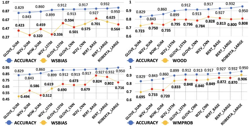
SUM) (Mikolov et al. 2013), GloVe Sum (GLOVE SUM)
                                                                (Pennington, Socher, and Manning 2014), Word2Vec LSTM
                                                                (W2V LSTM) (Hochreiter and Schmidhuber 1997), GloVe
                                                                LSTM (GLOVE LSTM), Word2Vec CNN (W2V CNN) (Le-
                                                                Cun, Bengio et al. 1995), GloVe CNN (GLOVE CNN),
                                                                BERT Base (BERT BASE) (Devlin et al. 2018), BERT
                                                                Large (BERT LARGE) with GELU (Hendrycks and Gim-
                                                                pel 2016b), and RoBERTa Large (ROBERTA LARGE) (Liu
                                                                et al. 2019), following a recent work on OOD Robustness
                                                                (Hendrycks et al. 2020). We analyze these models over two
Figure 1: Leveraging various evaluation metrics for leader-     movie review datasets: (i) SST-2 (Socher et al. 2013)– con-
board customization, depending on application require-          tains short movie reviews written by experts , and (ii) IMDb
ments. A robot in a manufacturing industry (Heyer 2010)–        (Maas et al. 2011)– has full-length lay movie reviews. We
which is a less risky environment, compared to say              train models on SST-2 and evaluate on both SST-2 and
healthcare– is unlikely to experience OOD data, computa-        IMDb. This setup ensures both IID (SST-2 test set) and OOD
tional constraints, and spurious bias. Thus accuracy can be     (IMDb) evaluation.
used for evaluation.
                                                                                  Metric Formulation
                                                                Based on our three-pronged quantification of difficulty, we
• We present a methodology to probe leaderboards and            adapt WOOD Score, and propose WSBias and WMProb.
  check if ‘better’ models are ranked higher.
• We propose alternate evaluation metrics for leaderboard       Ranking Samples:
  customization based on application specific requirements,     WSBias: Samples are ranked in decreasing order of the
  as shown in Figure 1. To the best of our knowledge, we        amount of spurious bias present. Algorithms 1 and 2 elab-
  are the first to propose leaderboard customization.           orate our approach to quantify the presence of spurious bias
• Our automatic sample annotation approach based on ‘dif-       across samples. Algorithm 1 is inspired from Curriculum
  ficulty’ indicators speeds up conventional evaluation pro-    Learning (Xu et al. 2020) and AFLite (Sakaguchi et al. 2019;
  cesses in all focus areas. For example, current OOD           Bras et al. 2020)– a recent technique for adversarial filtering
  generalization evaluation has the overhead of identifying     of dataset biases. Algorithm 2 incorporates bias related to
  OOD datasets corresponding to each dataset (without a         train and test set overlap (Lewis, Stenetorp, and Riedel 2020;
  consistent guideline distinguishing IID from OOD); OOD        Gorman and Bedrick 2019). Spurious bias here represents
  datasets might also have their own bias. Automatic an-        the ease (% of times) with which a sample is correctly pre-
  notation with STS allows for the identification of sample     dicted by linear models on top of RoBERTA features, irre-
  subsets that exhibit greater OOD characteristics, thus en-    spective of inter-model agreement used in measuring sample
  abling the use of in-house data splits for evaluation.        uncertainty (Lung et al. 2013; Chen, Sun, and Chen 2014).
                                                                WOOD: First, STS is calculated for each test set value with
• In order to help users select models best suited to their     respect to all train set samples. The STS values for the vary-
  applications we leverage ideas from software engineering      ing percentages of the train set data– ranging from the top
  (Beizer 1995; Ribeiro et al. 2020) and develop a tool pro-    1%-100% of the train set, in turn obtained by sorting the
  totype that interactively visualizes how model rankings       train set samples in descending order of STS against each
  change, based on flexible weight assignment to different      test set sample– with respect to each test set sample are av-
  splits of data.                                               eraged. The test samples are then sorted in descending order
• We perform a user study with experts from industries with     based on this averaged STS value. This is done as train-test
  different focus areas, and show that our prototype helps in   similarity is a task dependent hyper-parameter, which can
  calibrating the proposed metrics by reducing development      lead to either inductive or spurious bias (Mishra et al. 2020b;
  and testing effort on average by 41%.                         Gorman and Bedrick 2019).
• We show how the metrics reduce model performance in-          WMProb: Test samples are ranked in increasing order, based
  flation, minimizing the overestimation of capability of AI.   on the confidence of model prediction for that sample (i.e.,
                                                                the maximum softmax probability). WMProb differs from
• Our analysis yields some preliminary observations of the      the previous two metrics in that it operates on a model-
  strengths and weaknesses of 10 models; we recommend           dependent parameter, i.e., prediction confidence, rather than
  the use of appropriate evaluation metrics to do fair model    data-dependent (and model-independent) parameters.
  evaluation, thus minimizing the gap between research and
  the real world.                                               Split Formation and Weight Assignment:
                                                                The dataset is divided into splits, based either on user de-
                 Experimental Setup                             fined thresholds of the sample ‘difficulty’, or such that the
We experiment with ten different models– Bag-of-Words           splits are equally populated (Figure 2). Weight assignment
Sum (BOW-SUM) (Harris 1954), Word2Vec Sum (W2V                  for samples can either be done continuously, or split-wise
Algorithm 1: Bias within Test Set                                  Algorithm 2: Bias across Train and Test Set
  Result: Input: Testset T , Hyper-Parameters m, t,                  Result: Input: Trainset T r, Testset T , Z={Logistic
            Models M -[Logistic Regression, SVM],                              Regression, SVM Linear, SVM RBF, Naive
            Output: Spurious bias values B for each                            Bayes} and Output: Spurious bias values B
            sample S                                                           for each sample S
  Fine-tune RoBERTA on 10% of T and discard this                     Correct Evaluation Score C(S) = 0 for all S in T ;
   10% to get R and find R’s embeddings e;                           forall i ∈ Z do
  Evaluation Score E(S) = 0 for all S in R ;                             Train Model Z on T r and Evaluate on T ;
  Correct Evaluation Score C(S) = 0 for all S in R ;                     forall S ∈ T do
  forall i ∈ m do                                                             if model prediction is correct then
      Randomly select trainset of size t from R ;                                  C(S) = C(S) + 1
      while y < 2 do                                                          end
           Train M [y] on t using e and evaluate on rest                 end
             of R i.e. V ;                                           end
           forall S ∈ V do                                           forall S ∈ T do
                E(S) = E(S) + 1;                                         B(S) = C(S)/4
                if model prediction is correct then                  end
                    C(S) = C(S) + 1
                end
           end
      end                                                          Reward and Penalty Scores:
  end                                                              For each sample, d and e are respectively used as reward
  forall S ∈ T do                                                  and penalty multipliers of the assigned weights. This is done
      B(S) = C(S)/E(S)                                             in order to flexibly score each sample’s contribution to the
  end                                                              overall performance. For example, in Table 1, b1 = 1 for
                                                                   Split 1, b2 = 2 for Split 2. In Case 1, d = 1 and e = −1,
                                                                   meaning that in Split 1, correct and incorrect samples are as-
                                                                   signed scores of b1 ∗ d = 1 and b1 ∗ e = −1 respectively;
(Table 1). We also assign penalties to incorrectly answered        in Split 2, this follows as b2 ∗ d = 2 and b2 ∗ e = −2. d
samples by multiplying the assigned sample weights with            and e can vary, as shown across the other cases. We also use
penalty scores– as defined below.                                  quantified spurious bias, average STS, and maximum soft-
                                                                   max probability values for d and e, as shown in Cases 6-9.
Formalization:
Let D represent a dataset where T is the test set and T r is the              Leaderboard Probing Results
train set. B is the degree of bias / averaged STS value that a
                                                                   We use WSBias, WOOD, and WMProb Scores to probe
sample has, p is the model prediction, g is the gold annota-
                                                                   accuracy-based model performance/ranking. Based on the
tion, a (= 1 in our experiments) is a hyper-parameter used
                                                                   metric selected, we gain insights of models’ behavior over
in continuous weight calculation, b1 and b2 are the weights
                                                                   the two datasets considered, for different aspects of sample
assigned per split, th1 is the splitting parameter, either based
                                                                   ‘difficulty’, in terms of overall/split-wise performance.
on threshold value or equally populated splits. d and e are the
reward and penalty scores respectively, which are each mul-
                                                                   Range of Hyper-Parameters
tiplied with both b1 and b2 across splits. Here, Wcontinuous
and Wtwo−split refer to continuous and two-split weighting         We vary split numbers from 2 (as in Equation 2) to 7, which
schemes respectively.                                              are either equally populated, or formed based on equally
                                                                   spaced thresholds. We use the splits in combination with all
                                       a                           weighting schemes (as in Table 1) to calculate the metric val-
                      Wcontinuous =                         (1)
                                       B                           ues. Higher split numbers have additional weight and thresh-
                                                                  old hyper-parameters. For example, in the case of 4 splits,
                        b1 , if B > th1 (Split 1)                  we have weight hyper-parameters of b1 − b4 and threshold
         Wtwo−split =                                       (2)
                        b2 , otherwise (Split 2)                   hyper-parameters of th1 -th3 . We multiply each weight by
                                                                  d or e to assign sample scores. For example, the respective
                          d, if p = g                              correct/incorrect sample scores per split when b1 − b4 take
                  K=                                        (3)
                          e, otherwise                             values from 1 − 4, and d = 1, e = −0.5 are: +1/-0.5,+2/-
                          P
                              K ∗W                                 1,+3/-1.5,+4/-2. We also vary the bn hyper-parameter val-
               M etric = PT           ∗ 100                 (4)    ues along linear (additive and subtractive), logarithmic, and
                             T d∗W                                 square scales. Results for SST-2 show lesser extents of per-
   When B is the maximum softmax prediction probability,           formance inflation and ranking change– though these are
the value of Wcontinuous must be reciprocated in equation          still significant– which we attribute to SST-2 being the IID
1, and the split assignment must be swapped in equation 2.         dataset. We report results for 7 splits over the IMDb Dataset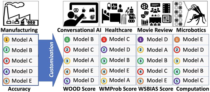
Split 1 Split 2
Case Description b1 b2 d e
Correct Incorrect Correct Incorrect
1 Reward = Penalty 1 2 1 -1 1 -1 2 -2
2 Reward Only 1 2 1 0 1 0 2 0
3 Penalty Only 1 2 0 -1 0 -1 0 -2
4 Reward > Penalty 1 2 1 -0.5 1 -0.5 2 -1
5 Penalty > Reward 1 2 0.5 -1 0.5 -1 1 -2
6 Continuous Weights 1/B 1/B 1 -1 1/B −1/B 1/B −1/B
7 Continuous Weights (*) B B 1 -1 B −B B −B
8 Reward = Penalty = B 1 2 1/B −1/B 1/B −1/B 2/B −2/B
9 Reward = Penalty = B (*) 1 2 B −B B −B 2B −2B
Table 1: Weighting Schemes Tested for WSBias, WOOD, and WMProb. Here, examples of weighting schemes for 2 splits are
shown, with Split 1 containing the ‘easy’ samples, and Split 2 containing the ‘hard’ samples. In Cases 6 and 8, 1/B refers to
quantified sample ‘difficulty’ and applies to WSBias and WOOD Score. In Cases 7 and 9, B is the ‘difficulty’ for WMProb.
below; we note that similar results are observed over differ- with WSBias are the least for transformer models, and the
ent hyper-parameter considerations for both datasets. most for word-averaging models. This follows from the in-
sight that transformer models predominantly fail on ‘eas-
WSBias ier’ samples, i.e., those which contain greater amounts of
GLOVE-LSTM Outperforms ROBERTA-LARGE in spurious bias. As ‘hard’ samples– with low spurious bias–
‘Easy’ Questions for Certain Splits: We see that when data are predominantly negatively scored for simpler models, the
is divided into 2-5 splits, ROBERTA-LARGE, despite hav- overall WSBias Score of the model decreases. This is be-
ing higher accuracy, has greater, equal, and lesser errors in cause the absolute weights assigned for those samples are
Splits 1 (easiest) - 3 respectively, than GLOVE-LSTM. This higher. Our findings thus indicate that simpler models are
indicates that ROBERTA-LARGE is unable to solve easy over-reliant on spurious bias.
samples efficiently.
Transformers Fail to Answer ‘Easy’ Questions: In Fig- WOOD
ure 2, in the parallel coordinates plot (PCP) model perfor-
mance values vary to a greater extent in Splits 1-3, and Model Performance Inflation Increases as % of Training
converge till they are near identical in Splits 6-7. Trans- Set Used to Calculate STS Increases: We note that over-
former models (BERT-BASE, BERT-LARGE, ROBERTA- all model performance increases when larger percentages of
LARGE) display poor performance on Split 1, with only the training set are used in the calculation of averaged STS
ROBERTA-LARGE having a marginally positive value. values for test samples. This is due to the corresponding de-
This may be attributed to catastrophic forgetting, which oc- crease in the variance of the averaged STS values (values
curs due to the larger quantities of data transformer models tend towards 0.5 at 100%).
are trained on to improve generalization. Split-wise Ranking Varies More for Lesser %s of Train-
Frequent Ranking Changes Across Splits for Word Av- ing Set Used to Calculate STS: Due to the decreased vari-
eraging and GLOVE Embedding Models: In the PCP, the ation effect of averaging STS values for higher percentages
occurrence of crossed/overlapping lines indicates frequent (> 50), there is less fluctuation in the split-wise distributions
ranking changes for the BOW-SUM, GLOVE-LSTM, and of incorrect predictions, especially in thresholded splits. As
GLOVE-CNN models over all the splits. This result is repli- a result, the split-wise model ranking changes more fre-
cated for all weighting schemes. quently when lower percentages are used for STS calcula-
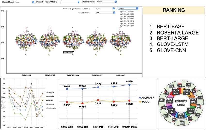
Significant Changes in Model Ranking: In the multi-line tion. In Figure 2 (25%), this is indicated by clear and fre-
chart (MLC) (Figure 3), the scores do not monotonically in- quent line crossings.
crease unlike the behavior seen in accuracy. There is a signif- Overall Ranking Changes Significantly for All %s of
icant change in model ranking, with 8/10 models changing Training Set Considered: There is significant ranking
positions, as indicated by the red dots. The concurrence of change irrespective of STS %, to a greater extent than with
significant ranking changes using both algorithms indicates WSBias. For example, in Figure 3, we see that (i) 9/10 mod-
that irrespective of model training, accuracy does not appro- els change their ranking position based on WOOD (calcu-
priately rank models based on spurious bias considerations. lated with 25% STS), and (ii) there is a decrease of 15% in
Significant Reduction in Model Performance Inflation: WOOD score values, with respect to accuracy. These respec-
The overall WSBias score values decrease by: (i) 25%-63% tively indicate that accuracy does not rank appropriately in
for Algorithm 1, and (ii) 11%-40% for Algorithm 2, with the context of model generalization, and also inflates model
respect to accuracy. This indicates that WSBias solves accu- performance on OOD datasets. These results are replicated
racy’s inflated model performance reporting. over all weight and STS % considerations.
Transformer Model Performance is the Least Inflated: W2V-CNN Beats Transformers in Most Splits: The trans-
We observe in the MLC that the performance drops seen former models are consistently surpassed by W2V-CNN in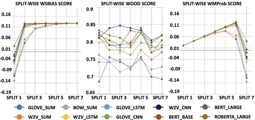
Figure 2: Split-wise results for each model using WSBias (based on Algorithm 1 – left), WOOD (based on top 25% STS
averaging – middle), and WMProb (right) are shown in the PCPs. Each vertical line indicates the data split considered (Split
1 – Easiest/Lowest Confidence, Split 7 – Hardest/Highest Confidence). Weighting scheme considered is Case 1, for 7 equally
populated splits on the IMDb dataset

Splits 2,3,4,6,7. W2V-CNN also beats transformers in over-         ment by ignoring model confidence, the influence of model
all WOOD Score; this is because transformers fail to solve         confidence is lesser compared to OOD characteristics and
samples with low STS (i.e., higher OOD characteristics, ab-        bias used in the other metrics. Similar results are observed
solute weight assignments),and are thus heavily penalized.         in other weight/split considerations.

WMProb                                                                                       Discussion
Some Models are Better Posed to Abstain than Oth-
ers: When splits are formed based on both threshold and            We find that GLOVE-LSTM efficiently utilizes spuri-
equal population constraints, the number of incorrect predic-      ous bias to solve ‘easy’ questions. Also, W2V-CNN has
tions is approximately equally distributed across splits for all   the highest capability for OOD generalization. While
models. In particular, ROBERTA-LARGE, BERT-LARGE,                  ROBERTA-LARGE has the highest number of correct pre-
and GLOVE-SUM display near-equal numbers of incor-                 dictions per split, it more or less uniformly distributes in-
rect samples at the ‘easiest’ (high confidence) and ‘hardest’      correct predictions across all splits (i.e., varying levels of
(low confidence) splits. On the other hand, BERT-BASE,             confidence). Therefore, if ROBERTA-LARGE is augmented
GLOVE-LSTM, and W2V-LSTM show near-monotonic de-                   with the capability seen in BERT-BASE, GLOVE-LSTM
crease in the number of samples correctly answered from            and W2V-LSTM of better correlation of prediction correct-
high to low confidence. For safety critical applications, mod-     ness with prediction confidence, then it may be better suited
els are made to abstain from answering if the maximum soft-        for safety critical applications. Additionally, our results over
max probability is below a specified threshold. If a lesser        both datasets show that transformers, in general, fail to solve
number of incorrect predictions (i.e., higher accuracy) is as-     ‘easy’ questions; the fact that simpler models solve easy
sociated with high model confidence, that model is preferred       questions more efficiently can be utilized to create ensem-
for deployment.                                                    bles, and subsequently, better architectures. Conducting fur-
Least Change in Ranking: The MLC (Figure 3) shows that             ther experiments on different datasets and tasks is a potential
out of the 3 metrics, accuracy most closely models WMProb,         future work to generalize these findings.
with 6/10 models changing ranking position; these changes
are local, with models moving up or down a single rank in                 Prototype for Leaderboard Probing and
three swapped pairs.                                                                  Customization
All Models Perform Poorly While Answering With High
Confidence: Unlike the other metrics, here we see that all         We develop an interactive tool prototype1 – leveraging WS-
models exhibit a sharp decrease in split-wise performance          Bias, WOOD, and WMProb– to help industry experts probe
in the last split, where prediction confidence is highest.         and customize leaderboards, as per their deployment sce-
Accuracy Least Inflates Model Performance in the Con-              nario requirements. The provision of a platform for such
text of Prediction Confidence: There is only a 5%-16%              structured analysis is aimed at helping experts select better
decrease in WMProb values when compared to accuracy, in-
                                                                      1
dicating that while accuracy inflates performance measure-                https://github.com/swarooprm/Leaderboard-Customization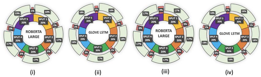
Figure 3: The MLCs shows the model performance based on Accuracy and WSBias (from Algorithms 1, 2) / WOOD / WMProb.
Here, the yellow dots indicate that the model’s ranking position is the same as that of accuracy, red dots indicate that there is a
change in ranking position. Weighting scheme considered is Case 1, for 7 equally populated splits on the IMDb dataset.

models, as well as reducing their pre-deployment develop-            from leaderboards (with accuracy as the metric, i.e., uniform
ment and testing effort. We evaluate this prototype in two           weighting, no penalty). In conventional selection, users have
stages– (i) Expert Review, and (ii) Detailed User Study.             to iteratively pick some models from the leaderboard, then
                                                                     test those models in their specific application (through test
Expert Review                                                        cases and deployment), until they find one that works effi-
We present an initial schematic, covering ten models over            ciently. Figure 4 summarizes user study results.
the SST-2 and IMDb datasets, to five software testing experts
(6+ years of work experience), each working in one of the            Feedback
focus areas illustrated in Figure 1. There is a shared belief
among experts that “the use of this tool will reduce testing         A total of 32 experts participated in the evaluation of our
time/effort by reducing the number of models initially vet-          prototype. On average, development and testing effort de-
ted” (P1, P4). Additionally, “... selecting good base models         crease of 41% is reported using our customized leader-
reduces testing times downstream the pipeline” (P3). Based           board approach, as opposed to conventional model selec-
on this initial feedback, we add a feature to custom-load            tion and testing approaches. This decrease is attributed to the
model results and data (as present in conventional software          prototype’s “... improvement for data collection time frames
testing platforms). This extends the utility of our prototype        and downstream testing since we know exactly where the
from the initial phase of probing and model selection, to ex-        model fails.”(P7). (P6) believes our prototype “can help in
tensive, iterative behavioral testing that occurs in later test-     creating model ensembles”, and (P8) that it will “help with
ing phases, prior to deployment.                                     the expedited development and testing of AI models... auto-
                                                                     suggested model edits through the visual interface would be
User Study                                                           interesting”. (P14, P31) say our prototype ... helps compare
We approach software developers and testing managers of              in-house and commercial model strengths and weaknesses.
several commercial product development teams (belong-                (P20) further attributes this facilitated comparison towards
ing to 9 companies) across all five focus areas. We first            enabling “...testing of various possible scenarios in deploy-
outline the basic intuitions behind the formulation of the           ment without writing test cases... we do not have to write
three metrics, and then provide users with our prototype.            separate test cases for stress testing”, and (P26) adds that
In the visual interface, users can interactively test vari-          “A big part of testing involves creating new datasets in the
ous splits (manual/random/automatic methods– i.e., equally           sandbox that mimic deployment scenarios. Dataset creation,
populated/thresholded splits) and weighting schemes (with            annotation, controlling quality, and evaluation are costly.
flexible penalty assignment, and discrete/continuous weight-         This tool’s unique method of annotating existing datasets
ing) of data for different metrics. The users are then asked         helps us significantly reduce previously spent effort.”. (P22)
to fill a Google Form, juxtaposing their prototype usage             suggests “... exploring the potential expansion of this tool to
with conventional model selection– refers to picking models          assist in customized functional testing of products”.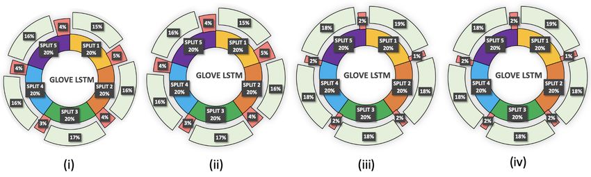
Figure 4: Reported Decreases in pre-deployment development and testing. Average : 40.791%

                     Related Works                               et al. 2019; Iyyer et al. 2018), intended to mislead models
Beyond Accuracy: CheckList, a matrix of general linguis-         (Jia et al. 2019). Our work, in contrast, deals with the ad-
tic capabilities and test types, has been introduced to enable   versarial attack of leaderboards. Ladder (Blum and Hardt
better model evaluation and address the performance over-        2015) has been proposed as a reliable leaderboard for ma-
estimation associated with accuracy (Ribeiro et al. 2020).       chine learning competitions, by preventing participants from
Alternate evaluation approaches such as model robustness         overfitting to holdout sets. Our objective is orthogonal to this
to noise (Belinkov and Bisk 2017), Perturbation Sensitiv-        as it focuses on customizing leaderboards based on applica-
ity Analysis–a generic evaluation framework detects un-          tion specific requirements in industry.
intended model biases related to named entities– (Prab-
hakaran, Hutchinson, and Mitchell 2019), and energy us-                                  Conclusion
age in models (Henderson et al. 2020) (promoting Green
AI (Schwartz et al. 2019; Mishra and Sachdeva 2020)) have        We present a method to adversarially attack leaderboards,
also been proposed. Our proposed idea of weighting samples       and utilize this to probe model rankings. We find that ‘bet-
based on ‘hardness’, is metric-independent, and can be used      ter’ models are not always ranked higher, and therefore pro-
to revamp other metrics beyond accuracy such as F1 Score.        pose new evaluation metrics that enable equitable model
Evaluation Metrics and Recommendations: The mis-                 evaluation, by weighting samples based on their hardness
alignment of automatic metrics with the gold standard of         from perspectives of data and model dependencies. We use
human evaluation for Text Generation has been studied in         these metrics to develop a tool prototype for leaderboard
several works (Mathur, Baldwin, and Cohn 2020; Sellam,           customization by adapting software engineering concepts.
Das, and Parikh 2020). Our work is orthogonal to these,          We perform a user study with experts from nine industries,
as we have no reference human evaluation, and our idea           having five different focus areas, and find that our prototype
of weighted metrics is task-independent. Evaluation met-         helps in calibrating the proposed metrics by reducing user
ric analysis has been used to provide recommendations            development and testing effort on average by 41%. Our met-
(Peyrard 2019) for gathering human annotations in speci-         rics reduce inflation in model performance, thus rectifying
fied scoring ranges (Radev et al. 2003). ‘Best practices’ for    overestimated capabilities of AI systems. Our results also
reporting experimental results (Dodge et al. 2019), the use      give preliminary indications of the strengths and weaknesses
of randomly generated splits (Gorman and Bedrick 2019),          of 10 models. We recommend the use of appropriate evalu-
and comparing score distributions on multiple executions         ation metrics to do fair model evaluation, thus minimizing
(Reimers and Gurevych 2017) have been recommended. Our           the gap between research and the real world. In the future,
work recommends the reporting of performance in terms of         we will expand our analysis to model ensembles, as they
the weighted metrics, along with accuracy, and their integra-    are seen to dominate leaderboards more often. Our equitable
tion as part of leaderboard customization.                       evaluation metrics can also be useful in competitions, and
Adversarial Evaluation: Adversarial evaluation tests the         we plan to expand our user study to competitions in future.
capability of systems to not get distracted by text added to     We hope the community expands the usage of such evalua-
samples in several different forms (Jia and Liang 2017; Jin      tion metrics to other domains, such as vision and speech.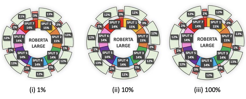
Ethics Statement                              of the Energy and Carbon Footprints of Machine Learning.
The broad impact of our work is as follows:                      arXiv preprint arXiv:2002.05651 .
                                                                 Hendrycks, D.; and Gimpel, K. 2016a. A baseline for detect-
Environmental Impact: Competitions and leaderboards in           ing misclassified and out-of-distribution examples in neural
general can have a negative impact on climate change, as         networks. arXiv preprint arXiv:1610.02136 .
increasingly complex models are trained and retrained, re-       Hendrycks, D.; and Gimpel, K. 2016b. Gaussian error linear
quiring more computation time. Our proposed method could         units (gelus). arXiv preprint arXiv:1606.08415 .
help teams reduce the exploration space to find a good
model, and thus help reduce that team’s overall carbon emis-     Hendrycks, D.; Liu, X.; Wallace, E.; Dziedzic, A.; Kr-
sions.                                                           ishnan, R.; and Song, D. 2020. Pretrained Transformers
Towards a Fair Leaderboard: Our definition of ‘diffi-            Improve Out-of-Distribution Robustness. arXiv preprint
culty’ can be extended based on several different perspec-       arXiv:2004.06100 .
tives. A viable application of this is a ‘fair’ customized       Heyer, C. 2010. Human-robot interaction and future indus-
leaderboard, where models having higher gender/racial bias       trial robotics applications. In 2010 IEEE/RSJ International
will be heavily penalized, preventing them from dominating       Conference on Intelligent Robots and Systems, 4749–4754.
leaderboards.                                                    IEEE.
Selecting the Best Natural Language Understanding
                                                                 Hochreiter, S.; and Schmidhuber, J. 1997. Long short-term
(NLU) Systems: NLU requires a variety of linguistic ca-
                                                                 memory. Neural computation 9(8): 1735–1780.
pabilities and reasoning skills. Incorporating these require-
ments systematically as ‘difficulties’ in our framework will     Iyyer, M.; Wieting, J.; Gimpel, K.; and Zettlemoyer, L.
enable better selection of top NLU systems.                      2018.      Adversarial example generation with syntacti-
                                                                 cally controlled paraphrase networks.        arXiv preprint
                       References                                arXiv:1804.06059 .
Beizer, B. 1995. Black-box testing: techniques for functional    Jia, R.; and Liang, P. 2017.          Adversarial Examples
testing of software and systems. John Wiley & Sons, Inc.         for Evaluating Reading Comprehension Systems. ArXiv
                                                                 abs/1707.07328.
Belinkov, Y.; and Bisk, Y. 2017. Synthetic and natural
noise both break neural machine translation. arXiv preprint      Jia, R.; Raghunathan, A.; Göksel, K.; and Liang, P. 2019.
arXiv:1711.02173 .                                               Certified Robustness to Adversarial Word Substitutions. In
                                                                 EMNLP/IJCNLP.
Blum, A.; and Hardt, M. 2015. The ladder: A reliable leader-
board for machine learning competitions. arXiv preprint          Jin, D.; Jin, Z.; Tianyi Zhou, J.; and Szolovits, P. 2019. Is
arXiv:1502.04585 .                                               BERT Really Robust? A Strong Baseline for Natural Lan-
                                                                 guage Attack on Text Classification and Entailment. arXiv
Bowman, S. R.; Angeli, G.; Potts, C.; and Manning, C. D.         arXiv–1907.
2015. A large annotated corpus for learning natural language
inference. arXiv preprint arXiv:1508.05326 .                     Kamath, A.; Jia, R.; and Liang, P. 2020.             Selective
                                                                 Question Answering under Domain Shift. arXiv preprint
Bras, R. L.; Swayamdipta, S.; Bhagavatula, C.; Zellers, R.;      arXiv:2006.09462 .
Peters, M. E.; Sabharwal, A.; and Choi, Y. 2020. Adversarial
Filters of Dataset Biases. arXiv preprint arXiv:2002.04108       LeCun, Y.; Bengio, Y.; et al. 1995. Convolutional networks
.                                                                for images, speech, and time series. The handbook of brain
                                                                 theory and neural networks 3361(10): 1995.
Chen, H.; Sun, J.; and Chen, X. 2014. Projection and uncer-
tainty analysis of global precipitation-related extremes using   Lewis, P.; Stenetorp, P.; and Riedel, S. 2020. Question and
CMIP5 models. International journal of climatology 34(8):        Answer Test-Train Overlap in Open-Domain Question An-
2730–2748.                                                       swering Datasets. arXiv preprint arXiv:2008.02637 .
Devlin, J.; Chang, M.-W.; Lee, K.; and Toutanova, K. 2018.       Liu, Y.; Ott, M.; Goyal, N.; Du, J.; Joshi, M.; Chen, D.;
Bert: Pre-training of deep bidirectional transformers for lan-   Levy, O.; Lewis, M.; Zettlemoyer, L.; and Stoyanov, V.
guage understanding. arXiv preprint arXiv:1810.04805 .           2019. Roberta: A robustly optimized bert pretraining ap-
                                                                 proach. arXiv preprint arXiv:1907.11692 .
Dodge, J.; Gururangan, S.; Card, D.; Schwartz, R.; and
Smith, N. A. 2019. Show Your Work: Improved Reporting            Lung, T.; Dosio, A.; Becker, W.; Lavalle, C.; and Bouwer,
of Experimental Results. In EMNLP/IJCNLP.                        L. M. 2013. Assessing the influence of climate model un-
                                                                 certainty on EU-wide climate change impact indicators. Cli-
Gorman, K.; and Bedrick, S. 2019. We need to talk about          matic change 120(1-2): 211–227.
standard splits. In Proceedings of the 57th annual meeting
of the association for computational linguistics, 2786–2791.     Maas, A. L.; Daly, R. E.; Pham, P. T.; Huang, D.; Ng, A. Y.;
                                                                 and Potts, C. 2011. Learning word vectors for sentiment
Harris, Z. S. 1954. Distributional structure. Word 10(2-3):      analysis. In Proceedings of the 49th annual meeting of the
146–162.                                                         association for computational linguistics: Human language
Henderson, P.; Hu, J.; Romoff, J.; Brunskill, E.; Jurafsky,      technologies-volume 1, 142–150. Association for Computa-
D.; and Pineau, J. 2020. Towards the Systematic Reporting        tional Linguistics.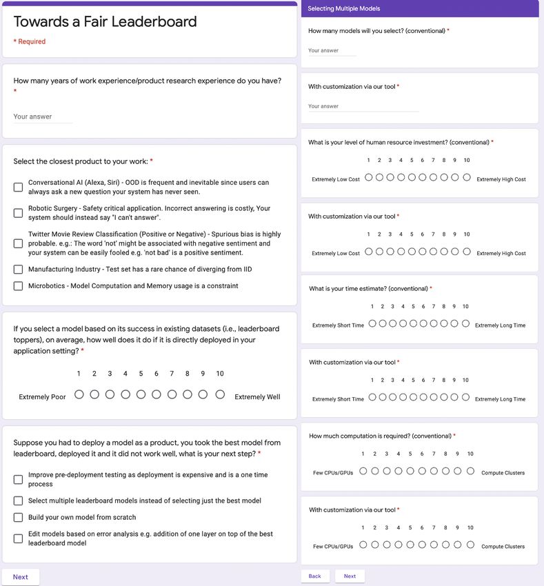
Mathur, N.; Baldwin, T.; and Cohn, T. 2020. Tangled up in       Socher, R.; Perelygin, A.; Wu, J.; Chuang, J.; Manning,
BLEU: Reevaluating the Evaluation of Automatic Machine          C. D.; Ng, A. Y.; and Potts, C. 2013. Recursive deep models
Translation Evaluation Metrics. In ACL.                         for semantic compositionality over a sentiment treebank. In
Mikolov, T.; Sutskever, I.; Chen, K.; Corrado, G. S.; and       Proceedings of the 2013 conference on empirical methods in
Dean, J. 2013. Distributed representations of words and         natural language processing, 1631–1642.
phrases and their compositionality. In Advances in neural       Torralba, A.; and Efros, A. A. 2011. Unbiased look at dataset
information processing systems, 3111–3119.                      bias. In CVPR 2011, 1521–1528. IEEE.
Mishra, S.; Arunkumar, A.; Bryan, C.; and Baral, C. 2020a.      Xu, B.; Zhang, L.; Mao, Z.; Wang, Q.; Xie, H.; and Zhang,
Our Evaluation Metric Needs an Update to Encourage Gen-         Y. 2020. Curriculum Learning for Natural Language Under-
eralization. ArXiv abs/2007.06898.                              standing. In Proceedings of the 58th Annual Meeting of the
                                                                Association for Computational Linguistics, 6095–6104.
Mishra, S.; Arunkumar, A.; Sachdeva, B. S.; Bryan, C.; and
Baral, C. 2020b. DQI: Measuring Data Quality in NLP.
ArXiv abs/2005.00816.                                                                1   Organization
Mishra, S.; and Sachdeva, B. S. 2020. Do We Need to Create      • More Split-Wise Results
Big Datasets to Learn a Task? In SUSTAINLP.                     • More Ranking Changes for Various Hyper-Parameter
Pennington, J.; Socher, R.; and Manning, C. D. 2014. Glove:       Considerations
Global vectors for word representation. In Proceedings of       • Visual Interface for Tool
the 2014 conference on empirical methods in natural lan-
guage processing (EMNLP), 1532–1543.                            • Google Form for User Study
Peyrard, M. 2019. Studying Summarization Evaluation Met-                      2    More Split-Wise Results
rics in the Appropriate Scoring Range. In ACL.
                                                                Please refer to Figures 5,6,7,8.
Prabhakaran, V.; Hutchinson, B.; and Mitchell, M. 2019.
Perturbation sensitivity analysis to detect unintended model         3   More Ranking Changes for Various
biases. arXiv preprint arXiv:1910.04210 .
                                                                         Hyper-Parameter Considerations
Radev, D.; Teufel, S.; Saggion, H.; Lam, W.; Blitzer, J.; Qi,   Please refer to Tables 2,3,4,5,6,7,8,9
H.; Celebi, A.; Liu, D.; and Drabek, E. F. 2003. Evaluation
challenges in large-scale document summarization. In Pro-
ceedings of the 41st Annual Meeting of the Association for
                                                                              4    Visual Interface for Tool
Computational Linguistics, 375–382.                             Please refer to Figure 9.
Rajpurkar, P.; Zhang, J.; Lopyrev, K.; and Liang, P. 2016.
Squad: 100,000+ questions for machine comprehension of
                                                                          5       Google Form for User Study
text. arXiv preprint arXiv:1606.05250 .                         The study covers cases where users find model performance
                                                                in real world scenarios to range from 1-8 (/10). The user
Recht, B.; Roelofs, R.; Schmidt, L.; and Shankar, V. 2019.      spread over the five application types is also balanced. Users
Do imagenet classifiers generalize to imagenet? arXiv           are specifically asked to initially select a product(s) closest
preprint arXiv:1902.10811 .                                     to their line of work from the following options: (i) Con-
Reimers, N.; and Gurevych, I. 2017. Reporting Score Distri-     versational AI (Alexa/Siri): OOD data is frequent and in-
butions Makes a Difference: Performance Study of LSTM-          evitable due to low control over user input, (ii) Robotic
networks for Sequence Tagging. ArXiv abs/1707.09861.            Surgery: Safety critical applications cannot afford incorrect
Ribeiro, M. T.; Wu, T.; Guestrin, C.; and Singh, S. 2020.       model answering, and require models to abstain if they are
Beyond Accuracy: Behavioral Testing of NLP models with          unable to answer, (iii) Twitter Movie Review Classification
CheckList. In ACL.                                              (Sentiment Analysis): Spurious Bias may play a significant
                                                                role in fooling a model due to the frequent repetition of cer-
Russakovsky, O.; Deng, J.; Su, H.; Krause, J.; Satheesh, S.;    tain words or patterns (e.g.: ‘not’ doesn’t necessarily indi-
Ma, S.; Huang, Z.; Karpathy, A.; Khosla, A.; Bernstein, M.;     cate negative sentiment), (iv) Manufacturing Industry: The
et al. 2015. Imagenet large scale visual recognition chal-      test set has a rare chance of diverging from IID, and (v) Mi-
lenge. International journal of computer vision 115(3): 211–    crobotics: Model computation and memory usage are im-
252.                                                            portant constraints. This is intended to allow users to map
Sakaguchi, K.; Bras, R. L.; Bhagavatula, C.; and Choi, Y.       the metrics discussed and rankings observed to specific real-
2019. Winogrande: An adversarial winograd schema chal-          world applications that they have worked on, where top-
lenge at scale. arXiv preprint arXiv:1907.10641 .               ranked leaderboard models were found to fail during test-
                                                                ing, if directly applied. Users are then asked to answer how
Schwartz, R.; Dodge, J.; Smith, N. A.; and Etzioni, O. 2019.    the time, computation, and resources spent in using conven-
Green ai. arXiv preprint arXiv:1907.10597 .                     tional leaderboards compares to using a customized, visu-
Sellam, T.; Das, D.; and Parikh, A. P. 2020. BLEURT:            ally augmented leaderboard with the new metric(s) of their
Learning Robust Metrics for Text Generation. In ACL.            choice, in terms of: (i) selection of multiple models, (ii)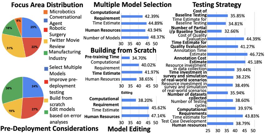
Figure 5: The inner-ring shows how 5 splits are formed in ROBERTA-LARGE and GLOVE-LSTM on the basis of thresholding
at bias score values (calculated with Algorithm 1) of 0.2, 0.4, 0.6, 0.8 for the IMDb (i,ii) and SST-2 (iii,iv) Datasets. The
outer-ring shows the proportion of correct (light-green) /incorrect (light-red) sample predictions per split.

Figure 6: The inner-ring shows how 7 equal splits are formed in ROBERTA-LARGE based on ranking using averaged STS
values of test set samples with respect to the Top 1% (i) ,10% (ii) ,100% (iii) of train set samples for the SST-2 dataset. The
outer ring shows the proportion of correct (light-green)/incorrect (light-red) predictions per split.

custom-building of a new model from scratch, (iii) editing
of an existing model, (iv) developing a testing strategy, and
(v) creation, collection, and annotation of data.
   Please refer to Figures 10,11,12,13,14.
Figure 7: Inner ring shows the sample distribution over 5 splits formed on the basis of: (i,iii) thresholding at averaged confi-
dence values of 0.2, 0.4, 0.6, 0.8, and (ii,iv) equal number of samples per split, for the SST-2 (iii,iv) and IMDb (i,ii) datasets
using confidence values of predictions by the GLOVE-LSTM model. The outer-ring shows the proportions of correct (light-
green)/incorrect (light-red) samples classified per split.

     Accuracy                                                          WOOD
      SST-2           7 Splits        6 Splits         5 Splits        4 Splits        3 Splits        2 Splits      Overall Score
    BOW SUM          W2V SUM       GLOVE SUM        GLOVE SUM       GLOVE SUM       GLOVE SUM       GLOVE SUM        GLOVE SUM
   GLOVE SUM       GLOVE SUM         W2V SUM          W2V SUM         W2V SUM         W2V SUM        BOW SUM           W2V SUM
     W2V SUM        W2V LSTM        W2V LSTM         BOW SUM         BOW SUM         BOW SUM          W2V SUM         BOW SUM
    W2V LSTM       GLOVE CNN       GLOVE CNN         W2V LSTM        W2V LSTM        W2V LSTM        W2V LSTM         W2V LSTM
   GLOVE CNN         W2V CNN        BOW SUM         GLOVE CNN       GLOVE CNN       GLOVE CNN      GLOVE LSTM       GLOVE LSTM
     W2V CNN        BOW SUM          W2V CNN          W2V CNN         W2V CNN      GLOVE LSTM       GLOVE CNN        GLOVE CNN
  GLOVE LSTM      GLOVE LSTM      GLOVE LSTM       GLOVE LSTM      GLOVE LSTM         W2V CNN         W2V CNN          W2V CNN
 ROBERTA LARGE   ROBERTA LARGE   ROBERTA LARGE    ROBERTA LARGE   ROBERTA LARGE   ROBERTA LARGE   ROBERTA LARGE       BERT BASE
   BERT LARGE       BERT BASE      BERT LARGE       BERT LARGE       BERT BASE      BERT LARGE      BERT LARGE       BERT LARGE
    BERT BASE      BERT LARGE       BERT BASE        BERT BASE      BERT LARGE       BERT BASE       BERT BASE     ROBERTA LARGE

Table 2: SST-2 : WOOD Score Results: STS calculated using the top 1%, 5%, 10%, 25%, 30%, 40%, 50%, 75%, 100% of the
training data, over equally populated splits. Results are the same for all weight schemes. Orange and red cells represent changes
in ranking. White and green cells represent no change in ranking.

     Accuracy                                                          WOOD
      IMDB            7 Splits        6 Splits         5 Splits        4 Splits        3 Splits        2 Splits      Overall Score
   GLOVE SUM       GLOVE SUM       GLOVE SUM        GLOVE SUM       GLOVE SUM       GLOVE SUM       GLOVE SUM        GLOVE SUM
     W2V SUM        BOW SUM         BOW SUM          BOW SUM         BOW SUM         BOW SUM          W2V SUM         BOW SUM
    BOW SUM          W2V SUM         W2V SUM          W2V SUM         W2V SUM         W2V SUM        BOW SUM           W2V SUM
    W2V LSTM      GLOVE LSTM      GLOVE LSTM         W2V LSTM        W2V LSTM        W2V LSTM        W2V LSTM        GLOVE CNN
  GLOVE LSTM       GLOVE CNN        W2V LSTM       GLOVE LSTM      GLOVE LSTM       GLOVE CNN      GLOVE LSTM         W2V LSTM
   GLOVE CNN        W2V LSTM       GLOVE CNN        GLOVE CNN       GLOVE CNN      GLOVE LSTM       GLOVE CNN       GLOVE LSTM
     W2V CNN     ROBERTA LARGE     BERT LARGE         W2V CNN       BERT LARGE        W2V CNN         W2V CNN        BERT LARGE
    BERT BASE      BERT LARGE    ROBERTA LARGE      BERT LARGE        W2V CNN       BERT LARGE      BERT LARGE     ROBERTA LARGE
   BERT LARGE        W2V CNN         W2V CNN      ROBERTA LARGE   ROBERTA LARGE   ROBERTA LARGE      BERT BASE        BERT BASE
 ROBERTA LARGE      BERT BASE       BERT BASE        BERT BASE       BERT BASE       BERT BASE    ROBERTA LARGE        W2V CNN

Table 3: IMDb : WOOD Score Results: STS calculated using the top 1%, 5%, 10%, 25%, 30%, 40%, 50%, 75%, 100% of the
training data, over equally populated splits. Results are the same for all weight schemes. Orange and red cells represent changes
in ranking. White and green cells represent no change in ranking.
Figure 8: Split-wise results for each model using bias scores from both algorithms are shown in the parallel coordinates plots
(PCP) on the upper half of the figure. Each vertical line indicates the data split considered (Split 1 –Easiest, Split 7 –Hardest).
The multi-line charts (MLC) show the model performance based on Accuracy and WSBIAS. Here, on the WSBIAS line, yellow
dots indicate that the model’s ranking position is the same as that of accuracy, red dots indicate that there is a change in ranking
position. Weighting scheme considered is Case 1, for 7 equal splits on the IMDb dataset.
Accuracy WOOD
SST-2 5 Splits 4 Splits 3 Splits 2 Splits
BOW SUM GLOVE SUM GLOVE SUM GLOVE SUM GLOVE SUM
GLOVE SUM W2V SUM W2V SUM W2V SUM BOW SUM
W2V SUM BOW SUM BOW SUM BOW SUM W2V SUM
W2V LSTM W2V LSTM W2V LSTM W2V LSTM W2V LSTM
GLOVE CNN GLOVE CNN GLOVE CNN GLOVE CNN GLOVE LSTM
W2V CNN W2V CNN W2V CNN GLOVE LSTM GLOVE CNN
GLOVE LSTM GLOVE LSTM GLOVE LSTM W2V CNN W2V CNN
ROBERTA LARGE ROBERTA LARGE ROBERTA LARGE ROBERTA LARGE ROBERTA LARGE
BERT LARGE BERT LARGE BERT BASE BERT LARGE BERT LARGE
BERT BASE BERT BASE BERT LARGE BERT BASE BERT BASE
Table 4: SST-2 : WOOD Score Results: STS calculated using the top 1%, 5%, 10%, 25%, 30%, 40%, 50%, 75%, 100% of the
training data, over equally spaced (between 0-1) thresholded splits. Results are the same for all weight schemes. Orange cells
represent changes in ranking. White cells represent no change in ranking.Accuracy WOOD
IMDB 5 Splits 4 Splits 3 Splits 2 Splits
GLOVE SUM GLOVE SUM GLOVE SUM GLOVE SUM GLOVE SUM
W2V SUM BOW SUM BOW SUM BOW SUM W2V SUM
BOW SUM W2V SUM W2V SUM W2V SUM BOW SUM
W2V LSTM W2V LSTM W2V LSTM W2V LSTM W2V LSTM
GLOVE LSTM GLOVE LSTM GLOVE LSTM GLOVE CNN GLOVE LSTM
GLOVE CNN GLOVE CNN GLOVE CNN GLOVE LSTM GLOVE CNN
W2V CNN W2V CNN BERT LARGE W2V CNN W2V CNN
BERT BASE BERT LARGE W2V CNN BERT LARGE BERT LARGE
BERT LARGE ROBERTA LARGE ROBERTA LARGE ROBERTA LARGE BERT BASE
ROBERTA LARGE BERT BASE BERT BASE BERT BASE ROBERTA LARGE
Table 5: IMDb : WOOD Score Results: STS calculated using the top 1%, 5%, 10%, 25%, 30%, 40%, 50%, 75%, 100% of the
training data, over equally spaced (between 0-1) thresholded splits. Results are the same for all weight schemes. Orange cells
represent changes in ranking. White cells represent no change in ranking.
Accuracy WSBIAS
SST-2 Algo 1 Regular Splits Algo 2 Regular Splits Algo 1 Continuous Weights Algo 2 Continuous Weights Algo 1 Threshold Splits Algo 2 Threshold Splits
BOW SUM W2V-SUM GLOVE-SUM GLOVE-SUM GLOVE-SUM W2V-SUM GLOVE-SUM
GLOVE SUM W2V-LSTM BOW-SUM W2V-LSTM W2V-LSTM W2V-LSTM BOW-SUM
W2V SUM GLOVE-SUM W2V-SUM BOW-SUM BOW-SUM GLOVE-SUM W2V-SUM
W2V LSTM BOW-SUM W2V-LSTM W2V-SUM W2V-SUM BOW-SUM W2V-LSTM
GLOVE CNN GLOVE-CNN GLOVE-CNN GLOVE-CNN GLOVE-CNN GLOVE-CNN GLOVE-CNN
W2V CNN ROBERTA-LARGE W2V-CNN W2V CNN W2V CNN ROBERTA-LARGE W2V-CNN
GLOVE LSTM W2V-CNN GLOVE-LSTM GLOVE LSTM GLOVE LSTM W2V-CNN GLOVE-LSTM
ROBERTA LARGE GLOVE-LSTM ROBERTA-LARGE ROBERTA LARGE ROBERTA LARGE GLOVE-LSTM ROBERTA-LARGE
BERT LARGE BERT-LARGE BERT-LARGE BERT LARGE BERT LARGE BERT-LARGE BERT-LARGE
BERT BASE BERT-BASE BERT-BASE BERT BASE BERT BASE BERT-BASE BERT-BASE
Table 6: SST-2 : WSBIAS Score Results: Calculated using bias scores over 7,6,5,4,3,2 splits and overall score. Results are the
same for all weight schemes. Orange cells represent changes in ranking. White cells represent no change in ranking.
Accuracy WSBIAS
IMDB Algo 1 Regular Splits Algo 2 Regular Splits Algo 1 Continuous Weights Algo 2 Continuous Weights Algo 1 Threshold Splits Algo 2 Threshold Splits
GLOVE SUM W2V-SUM GLOVE SUM GLOVE SUM GLOVE SUM W2V-SUM GLOVE SUM
W2V SUM W2V-LSTM BOW SUM W2V SUM W2V SUM W2V-LSTM BOW SUM
BOW SUM GLOVE-SUM W2V SUM BOW SUM BOW SUM GLOVE-SUM W2V SUM
W2V LSTM BOW-SUM W2V LSTM W2V LSTM W2V LSTM BOW-SUM W2V LSTM
GLOVE LSTM GLOVE-CNN GLOVE CNN GLOVE LSTM GLOVE LSTM GLOVE-CNN GLOVE CNN
GLOVE CNN ROBERTA-LARGE W2V CNN GLOVE CNN GLOVE CNN ROBERTA-LARGE W2V CNN
W2V CNN W2V-CNN GLOVE LSTM W2V CNN W2V CNN W2V-CNN GLOVE LSTM
BERT BASE GLOVE-LSTM ROBERTA LARGE BERT BASE BERT BASE GLOVE-LSTM ROBERTA LARGE
BERT LARGE BERT-LARGE BERT LARGE BERT LARGE BERT LARGE BERT-LARGE BERT LARGE
ROBERTA LARGE BERT-BASE BERT BASE ROBERTA LARGE ROBERTA LARGE BERT-BASE BERT BASE
Table 7: IMDb : WSBIAS Score Results: Calculated using bias scores over 7,6,5,4,3,2 splits and overall score. Results are the
same for all weight schemes. Orange cells represent changes in ranking. White cells represent no change in ranking.Accuracy WMPROB
SST-2 Equal Splits Threshold Splits
BOW SUM GLOVE-SUM BOW SUM
GLOVE SUM BOW-SUM GLOVE SUM
W2V SUM W2V-SUM W2V SUM
W2V LSTM W2V-LSTM W2V LSTM
GLOVE CNN GLOVE CNN GLOVE CNN
W2V CNN W2V CNN W2V CNN
GLOVE LSTM GLOVE LSTM GLOVE LSTM
ROBERTA LARGE ROBERTA LARGE ROBERTA LARGE
BERT LARGE BERT LARGE BERT LARGE
BERT BASE BERT BASE BERT BASE
Table 8: SST-2 : WMPROB Score Results: Over 7,6,5,4,3,2 splits and overall score. Results are the same for all weight schemes.
Orange cells represent changes in ranking. White cells represent no change in ranking.
Accuracy WMPROB
IMDB Equal Splits Threshold Splits
GLOVE SUM GLOVE-SUM GLOVE-SUM
W2V SUM W2V-SUM BOW-SUM
BOW SUM BOW-SUM W2V SUM
W2V LSTM W2V-LSTM W2V-LSTM
GLOVE LSTM GLOVE-CNN GLOVE-CNN
GLOVE CNN W2V-CNN GLOVE-LSTM
W2V CNN GLOVE-LSTM W2V CNN
BERT BASE BERT-LARGE BERT-LARGE
BERT LARGE BERT-BASE BERT-BASE
ROBERTA LARGE ROBERTA-LARGE ROBERTA-LARGE
Table 9: IMDb : WMPROB Score Results:Over 7,6,5,4,3,2 splits and overall score. Results are the same for all weight schemes.
Orange cells represent changes in ranking. White cells represent no change in ranking.Figure 9: Visual Interface used in User Study: The user selects the metric, number of models to analyze, dataset, weight scheme, % of train samples to calculate average STS (if metric is WOOD), and the number (and basis–continuous, thresholded, equally populated, manually selected) splits. Based on this, a series of parallel beeswarm plots are generated. x-axis comprises of the models used, and y-axis of the ‘difficulty’ (here, based on STS) of the samples (so sample points at higher y-values are easy samples). The coloring is based on the split the sample belongs to, and the size indicates if the sample is correctly(larger) or incorrectly (smaller) classified. A PCP and MLC for the points is automatically generated. On hover over a sample, based on the model (i.e., corresponding x-coordinate), the sunburst chart (bottom right) for the model is generated. Finally, the new ranking based on the metric selected is displayed.
Figure 10: Google Form used for Survey
Figure 11: Google Form used for Survey
Figure 12: Google Form used for Survey
Figure 13: Google Form used for Survey
Figure 14: Google Form used for Survey
You can also read