Physics-based Reconstruction Methods for Magnetic Resonance Imaging
←
→
Page content transcription
If your browser does not render page correctly, please read the page content below
Physics-based Reconstruction Methods for
                                                     Magnetic Resonance Imaging
arXiv:2010.01403v1 [eess.IV] 3 Oct 2020

                                            Xiaoqing Wang1,2 , Zhengguo Tan1,2 , Nick Scholand1,2 , Volkert
                                                          Roeloffs1 , Martin Uecker1,2,3,4
                                              1 Institute for Diagnostic and Interventional Radiology, University Medical Center
                                                                         Göttingen, Göttingen, Germany
                                          2 German Centre for Cardiovascular Research (DZHK), Partner Site Göttingen, Göttingen,

                                                                                     Germany
                                            3 Cluster of Excellence “Multiscale Bioimaging: from Molecular Machines to Networks of

                                                    Excitable Cells” (MBExC), University of Göttingen, Göttingen, Germany
                                           4 Campus Institute Data Science (CIDAS), University of Göttingen, Göttingen, Germany

                                                                       30. September 2020

                                                                                Abstract
                                                   Conventional Magnetic Resonance Imaging (MRI) is hampered by long
                                               scan times and only qualitative image contrasts that prohibit a direct com-
                                               parison between different systems. Instead of assuming a fixed Fourier
                                               relationship, model-based reconstructions explicitly model the physical
                                               laws that govern the MRI signal generation. By formulating image re-
                                               construction as an inverse problem, quantitative maps of the underlying
                                               physical parameters can then be extracted directly from efficiently ac-
                                               quired k-space signals without intermediate image reconstruction – ad-
                                               dressing both shortcomings of conventional MRI at the same time. This
                                               review will discuss basic concepts of model-based reconstructions and re-
                                               port about our experience in developing several model-based methods over
                                               the last decade using selected examples.
                                               Keywords: Magnetic Resonance Imaging, model-based reconstruction,
                                               inverse problems

                                             Submitted to Philosophical Transactions of the Royal Society A.
                                             Correspondence to: Martin Uecker, email: martin.uecker@med.uni-goettingen.de

                                                                                     1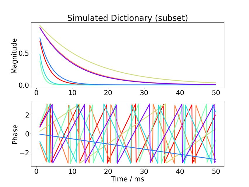
1    Introduction
First physics-based reconstruction methods for parametric mapping appeared
in the literature more than a decade ago [1, 2, 3] and constitute now a major
research area in the field of Magnetic Resonance Imaging (MRI). [4, 5, 6, 7, 8, 9,
10, 11, 12] Model-based reconstruction is based on modelling the physics of the
MRI signal and has been used, for example, to estimate T1 [13, 5, 8, 7, 12, 14],
T2 relaxation [3, 15, 9, 16], for T2? estimation and water-fat separation [17, 18,
19, 20], as well as for quantification of flow [10] and diffusion [21, 22]. Quantita-
tive maps of the underlying physical parameters can then be extracted directly
from the measurement data without intermediate image reconstruction. This di-
rect reconstruction has two major advantages: First, the full signal is described
by a model based on few parameter maps only and intermediate image recon-
struction is waived. This renders model-based techniques much more efficient in
exploiting the available information than conventional two-step methods. Sec-
ond, as a specific signal behaviour is no longer required for image reconstruction,
MRI sequences can now be designed that have an optimal sensitivity to the pa-
rameters of interest. Once the underlying physical parameters are estimated,
arbitrary contrast-weighted images can be generated synthetically by evaluating
the signal model for a specific sequence and acquisition parameters.

2    MRI Signal
In typical MRI experiments, the proton spins are polarized by bringing them
into a strong external field. The spins then start to precess with a character-
istic Larmor frequency and can be manipulated using additional on-resonant
radio-frequency pulses and further gradient fields. The dynamical behaviour of
the magnetization is described by the Bloch-Torrey equations that describe the
physics of magnetic resonance including effects from relaxation, flow and diffu-
sion. As a fully computer-controlled imaging method, MRI is extremely flexible
and the underlying physics enables access to a variety of tissue and imaging sys-
tem specific parameters such as relaxation constants, flow velocities, diffusion,
temperature, magnetic fields, etc.
    The measured MRI signal corresponds to the complex-valued transversal
magnetization M = Mx + iMy which is obtained by quadrature demodulation
from the voltage induced in the receive coils. In a multi-coil experiment this sig-
nal is proportional to the transversal magnetization weighted by the sensitivity
of each receive coil:            Z
                         yj (t) = cj (~r) M (x, B, t, ~r) d~r                   (1)

Here, cj is the complex-valued sensitivity of the jth coil and M the complex-
valued transversal magnetization at time t and position ~r. The magnetization
depends on some physical parameters x and the externally controlled magnetic
fields B(t, ~r), i.e. gradient fields and radio-frequency pulses, and can be obtained

                                         2
coil sensitivities

                          physics
   parameter maps         model

                                     signal
                                    evolution

Figure 1: The forward operator F can be formally factorized into operator M
that describes the spin physics, the multiplication with the coil sensitivities C,
the (non-uniform) Fourier transform F, and a sampling operator P.

by solving the Bloch-Torrey equations (or, if motion of spins can be neglected,
by solving the Bloch equations at each point).
     While equation 1 can be exploited directly for model-based reconstruction
[23], many other model-based methods use some simplifying approximations
to reduce the computational complexity. Often, segmentation in time is used
by assuming that the magnetization is constant around certain time points, e.g.
around echo times T En with n ∈ 1, . . . , N . The effect of magnetic field gradients
can then be separated out into a phase term which is defined by the k-space
trajectory ~k(t). This separation often allows the use of simplified models for
the magnetization and, more importantly, the use of fast (non-uniform) Fourier
transform algorithms for the gradient-encoding term. We derive the following -
still very generic - model:
                                Z
                                        ~
                      yn,j (t) = ei2π~r·k(t) cj (~r)M (x, tn , ~r)d~r             (2)

Based on this model, we define a nonlinear forward operator F : x 7→ y that
maps the unknown parameters x to the acquired data y (see Fig. 1).
    The defining feature of physics-modelling reconstruction is the addition of a
signal model M into the forward operator F . The specific signal model depends
on the applied sequence protocol and specifies which tissue and/or hardware
characteristics can be estimated. Often, an analytical model can be derived
from the Bloch equations using hard-pulse approximations. For many typical
MRI sequences important parameter dependencies are exponentials. Table 1
lists some of these analytical signals models.
If the applied sequence protocol does not lend itself to an analytical signal ex-
pression, the Bloch equations need to be integrated as signal model directly.

                                                3
parameter           sequence type               signal
        relaxation rate R1    inversion recovery   a − (1 + a) · e−tn R1/a
        relaxation rate R2        spin-echo                 e−R2 tn
                                                                  ∗
        relaxation rate R2?     gradient-echo               e−R2 tn
             field B0           gradient-echo             ei2π·fB0 tn
          chemical shift        gradient-echo
                                                          P i2πfp tn
                                                           pe
                                                                  ~
          flow velocity ~v     bipolar gradient             ei~v·Vn
                                                             ~T
        diffusion tensor D     bipolar gradient            e−bn Dbn

Table 1: Basic analytical signal models for physical parameter dependencies in
common MRI sequences.

This integration becomes challenging for iterative reconstructions, because of
the estimation of the signals derivatives. Current techniques exploit finite dif-
ference methods [9, 23] or sensitivity analysis of the Bloch equations [24].

3    Nonlinear Reconstruction
Using a nonlinear forward operator F : x 7→ y that maps the unknown param-
eters x to the acquired data y, we can formulate the image reconstruction as a
nonlinear optimization problem:
                                                      X
                x̂ = argmin kF (x) − yk22 + λQ(xc ) +   λi Ri (x)          (3)
                        x
                                                      i

Data fidelity is ensured by kF (x) − yk22 and regularization terms Ri can be
added to introduce prior knowledge. This framework is very general, combin-
ing parallel imaging, compressed sensing, and model-based reconstruction in
a unified reconstruction. Often the coil sensitivities are estimate before, but
they could also be included as unknowns in x. Paired with suitable sampling
schemes, this yields fully calibrationless methods that do not require additional
calibration scans [12, 25, 26, 10, 27, 28]. Moreover, model-based reconstructions
allow a direct application of sparsity-promoting regularizations to the physical
parameters for performance improvement [3, 6, 22, 12].
    However, the high non-convexity of model-based reconstruction makes this
method sensible to the initial guess and relative scaling of the derivatives of
each parameter map. These issues can often be addressed with a reasonable
initial guess and a proper preconditioning. Algorithms to solve the nonlinear
inverse problems include gradient descent, the variable projection methods [29],
the method of nonlinear conjugate gradient [30], Newton-type methods [31]
where the nonlinear problem is linearized in each Newton step and the linearized

                                       4
subproblem is solved using the method of conjugate gradients, FISTA [32] or
ADMM[33], or alternate minimization [6].
  Sequence   Flip Angle    TR/TE/∆TE           Bandwidth    Matrix       Spokes       TA    FOV   Slice
                 °               ms             Hz/px                                  s    mm    mm
 IR-FLASH        6           4.10 / 2.58          630      256 × 256      1020        4     192    5
  ME-SE       90/180      2000 / 9.9 / 9.9        390      256 × 256     25 × 16      80    192    3
 ME-FLASH        5        9.81 / 1.31 / 1.23     1090      200 × 200     33 × 7       0.3 1 320    5
 PC-FLASH       10           4.46 / 2.96         1250      210 × 210      2×7         15    320    5
  fmSSFP2       15            4.5 / 2.25          840      192 × 192   4 × 101 × 40   137   192    1
 1
     acquisition time per frame
 2
     3D Stack-Of-Stars sequence with 40 partitions (1000 prep scans)

Table 2: Detailed parameters of MR sequences capable of mapping physical
parameters listed in Table 1.
   Data for the following examples was obtained on a Siemens Skyra 3T scan-
ner (Siemens Healthcare GmbH, Erlangen, Germany) from volunteers without
known illness after obtaining written informed consent and with approval of the
local ethics committee. Acquisition parameters can be found in Table 2. The
images were reconstructed using the BART toolbox [34].

3.1     T1 and T2 Mapping
For T1 mapping, a inversion-recovery (IR) FLASH sequence was used. Following
a non-selective inversion pulse, data was continuously acquired using a radial
FLASH readout with a tiny golden angle (≈ 23.63◦ ) between successive spokes.
The magnetization signal M (t) for single-shot radial IR-FLASH reads
                                                                 ∗
               Mtk (~r) = Mss (~r) − Mss (~r) + M0 (~r) · e−tk ·R1 (~r)    (4)


with Mss the steady-state magnetization, M0 the equilibrium magnetization,
and R1∗ the effective relaxation rate. tk is the inversion time which is defined as
the center of each acquisition window.
    A radial multi-echo spin echo (ME-SE) sequence was employed for T2 map-
ping. Data was acquired with 25 excitations and 16 echoes. The golden angle
(≈ 111.25◦ ) was used between successive radial spokes. The magnetization sig-
nal M (t) for radial multi-echo spin echo at echo time tk follows an exponential
decay Mtk (~r) = M0 · e−tk ·R2 (~r) with M0 the spin density map, R2 = 1/T2 the
transverse relaxation rate. This simple exponential model does not take stim-
ulated echoes into account, but a more complicated analytical model exits for
this case [35].
    Quantitative parameter maps for both acquisitions are estimated using the
nonlinear model-based reconstruction. I.e., the estimation of parameter maps
(Mss , M0 , R1∗ )T or parameter maps (M 0, R2 )T , respectively, and coil sensitivity
maps (c1 , . . . , cN )T is formulated as a nonlinear inverse problem with a joint
`1 -Wavelet regularization applied to the parameter maps and the Sobolev norm
to the coil sensitivity maps. This nonlinear inverse problem is then solved by

                                                   5
(A) EstimatedTT11
Estimated EstimatedT
Estimated T12
5 6 1.8 Ground Truth 0.18 Ground Truth
4 10 7
1.4 0.14
3 1.0 0.10
9
1
2 8 0.6 0.06
0.2 0.02
1 2 3 4 5 6 7 8 9 10 1 2 3 4 5 6 7 8 9 10
0.4 0.8 1.2 1.6 2.0 0 0.05 0.10 0.15
0
Tubes Tubes
T1 / s T2 / s
(B) T1 / s
2.0
1.6
1.2
0.8
0.4
Mss M0 R 1* T1 0
T2 / s
0.15
0.10
0.05
M0 R2 T2 0
Figure 2: (A). (Leftmost) Model-based reconstructed T1 map and (left mid-
dle) the ROI-analysed quantitative T1 values for the numerical phantom using
the single-shot IR radial FLASH sequence. (Right middle and rightmost) Simi-
lar results for T2 mapping using the multi-echo spin-echo sequence. (B). (Top)
The reconstructed parameter maps (Mss , M0 , R1∗ )T for the T1 model and (bot-
tom) (M0 , R2 )T for the T2 model with the corresponding T1 / T2 maps in the
rightmost column.
the IRGNM-FISTA algorithm [12]. After estimation of the parameters T1 and
T2 maps can be calculated.
To evaluate the quantitative accuracy of the model-based methods, numeri-
cal phantoms with different T1 relaxation times (ranging from 200 ms to 2000
ms with a step size of 200 ms for each tube, and 3000 ms for the background),
T2 relaxation times (ranging from 20 ms to 200 ms with a step size of 20 ms for
each tube, and 1000 ms for the background) were simulated, respectively. The
k-space data were derived from the analytical Fourier representation of an el-
lipse assuming an array of eight circular receiver coils surrounding the phantom
without overlap.
Fig. 2 (A) presents the estimated T1, T2 maps and the corresponding ROI-
analyzed quantitative values for the numerical phantom using model-based re-
constructions. Good quantitative accuracy is confirmed for both model-based
6Water Fat R2* B0
Figure 3: Real-time liver images acquired during free-breathing using a radial
multi-echo (ME) FLASH sequence. Model-based reconstruction directly and
jointly estimates separated water and fat images, as well as R2? and B0 field
maps.
T1 and T2 mapping methods. Fig. 2 (B) demonstrates model-based recon-
structed three and two physical parameter maps, the corresponding T1 and T2
maps for the retrospective T1 and T2 models on human brain studies. More-
over, synthetic images were computed for all inversion/echo times and the image
series were then converted into movies showing the contrast changes in the sup-
plementary Videos 1 and 2.
3.2 Water/Fat Separation and R2∗ Mapping
Quantitative T2∗ mapping can be achieved via multi-echo gradient-echo sam-
pling. With prolonged echo-train readout, the acquired multi-echo signal fol-
lows, ∗
Mn = ρ · e−R2 ·TEn · ei2π·fB0 ·TEn (5)
where R2∗ and fB0 is the inverse of T2∗ and B0 field inhomogeneity, respectively.
TEn denotes the nth echo time. On the other hand, when the imaging voxel
contains distinct protons resonating at different frequencies, the magnetization
ρ can be split into multiple compartments. For instance, chemical shift between
water and fat induces phase modulation, therefore,
X ∗
Mn = (W + F · ei2πfp ·TEn ) · e−R2 ·TEn · ei2π·fB0 ·TEn (6)
p
where W and F are the water and fat magnetization, respectively. fp is the pth
fat-spectrum peak frequency. In practice, usually the 6-peak fat spectrum [36]
is used.
Here, a multi-echo (ME) radial FLASH sequence [28] was used to acquire
liver data during free breathing. The Sobolev-norm weight was applied to the B0
field inhomogeneity and coil sensitivity maps. Joint `1-Wavelet regularization
was applied to other parameter maps. As shown in Figure 3 and supplementary
7Video 3, high-quality respiratory-resolved water/fat separation as well as R2∗ and
fB0 maps can be achieved even with undersampled multi-echo radial acquisition
(33 spokes per echo and 7 echoes in total).
3.3 Phase-Contrast Velocity Mapping
In phase-contrast flow MRI, velocity-encoding gradients (i.e. bipolar gradients
with equal area but opposite polarity) are used to encode flow-induced phases.
Flowing spins with constant velocities during the bipolar gradient result in net
phase (proportional to the product between the gradient area and velocity),
whereas static spins result in zero phase. However, MR signal is in general
complex-valued due to the use of receiver coils. To compute the quantitative
velocity maps, a reference measurement without flow-encoding gradients is re-
quired such that the phase difference between the reference and flow-encoded
measurement excludes the background phase. Therefore, the mathematical
modelling of the phase-contrast flow MRI signal can be written as
~
Mk = ρ · ei~v·Vk . (7)
~v is the velocity and Vk is the velocity-encoding for the kth measurement. For
through-plane velocity mapping, V ~0 = 0 for the reference and V1 = π/VENC
the velocity-encoded measurement perpendicular to the imaging plane, respec-
tively. Here, VENC is the maximum measurable velocity in the unit of cm s−1
and inversely proportional to the first moment of the bipolar velocity-encoding
gradient. ρ is the shared anatomical image between the two measurements.
Multi-dimensional velocity mapping can be used as in 4D flow MRI [37]. Multi-
dimensional mapping was also used for real-time imaging of flow with model-
based reconstruction [38].
A phase-contrast flow MRI sequence with radial sampling and through-plane
velocity-encoding gradient was used to measure the in-vivo aortic blood flow ve-
locities. Two types of reconstructions were performed: model-based reconstruc-
tion [10, 27] based on the model in 7, and a parallel imaging reconstruction on
both reference and flow-encoded measurements followed by a phase-difference
computation. Fig. 4 shows the reconstructed velocity map from the model-
based reconstruction and phase-difference computation. Supplementary Video
4 displays the dynamic velocity maps of the whole 15-second scan. The later
approach employs parallel imaging reconstruction on the reference and the flow-
encoding measurement separately and then computes the phase difference be-
tween the reconstructed reference and flow-encoded images. With the direct
regularization on the phase-difference map, the proposed model-based recon-
struction is able to largely remove background random phase noise.
4 Linear Subspace Reconstruction
In contrast to nonlinear models, in linear subspace methods the signal curves
t 7→ M (x, t, ~r) are approximated using a linear combination of basis functions
8Model-based
Phase Difference
Figure 4: Comparison between (top) the model-based reconstruction and (bot-
tom) the conventional phase-difference reconstruction. A section crossing the
ascending and descending aorta was selected as the imaging slice. Displayed im-
ages are (left) anatomical magnitude image and (right) phase-contrast velocity
map at systole. With direct phase-difference regularization, the model-based
reconstruction largely reduces random background phase noise in the velocity
map.
9[39, 40, 41, 42, 43, 44] , i.e.
X
M (x, t, ~r) ≈ as (~r)Bs (t) . (8)
s
The linear basis functions Bs (t) can be generated by simulating a set of repre-
sentative signal curves for a range of parameter and performing a singular value
decomposition to obtain a good representation.
With known coil sensitivities, this leads to a linear inverse problem for the
subspace coefficients:
X
â = argmin ky − PF CBak22 + λi Ri (x) (9)
a
i
After reconstruction of the subspace coefficients as , the parameters x need
to be obtained in a separate step. This can be achieved by predicting complete
magnetization maps for all time points and fitting a nonlinear signal model.
This can be done point-wise, so is much easier than doing a full nonlinear
reconstruction. Still, for multi-parametric mapping efficient techniques to map
between coefficients and parameters are required [44].
Linear subspace methods have several advantages. Linear subspace models
linear problems without local minima. Due to their linearity, they also inher-
ently avoid model violations stemming from partial volume effects. Because
the matrix multiplication with the basis and other operations commute, they
admit a computationally advantageous formulation that allows computation in
the subspace [45, 41].
4.1 T1 Mapping
Alternatively, T1 maps were also reconstructed using the subspace method.
Similar to [43], the T1 dictionary was constructed using 1000 different 1/R1∗
values linearly range from 5–5000 ms, combining with 100 Mss values from
0.01 · M0 to M0 . This results in 100,000 exponential curves in the dictionary.
A subset of such a dictionary is shown in Fig. 5 (left). The other parame-
ters are TR = 4.10 ms, 20 spokes per frame, 51 frame in total. The simulated
curves are highly correlated and can be represented by only a few principle com-
ponents Fig. 5. For easier comparison, the subspace-constraint reconstruction
used the coil sensitivity maps estimated using model-based T1 reconstruction.
The resulting linear problem was then solved using conjugate gradient or FISTA
algorithm in BART. The coefficient maps were then projected back to image
series where the 3-parameter fit is applied for each voxel according to equation
(4).
Fig. 6 (A) shows estimated phantom T1 maps using a variant number of
complex coefficients of the linear subspace-based reconstruction with L2 regu-
larization. Lower number of coefficients causes bias for quantitative T1 mapping
(especially for tubes with short T1s) while higher number of coefficients brings
noise in the final T1 maps. Therefore 4 coefficient maps were chosen to com-
promise between quantitative accuracy and precision. Fig. 6 (B) compares the
10(A) Inversion Recovery Signal Simulation
(B) Multi-Gradient-Echo Signal Simulation
Figure 5: Demonstration of subspace-based methods for (A) single-shot
inversion-recovery and (B) multi-gradient-echo signal, respectively. (Left) Sim-
ulated (top) T1 relaxation and (bottom) T2∗ relaxation and off-resonance phase
modulation curves. (Center) Plot of the first 30 principle components. (Right)
The temporal subspace curves that can be linearly combined to form (top) T1
relaxations and (bottom) multi-gradient-echo relaxations.
11Linear Subspace Model
(A) Reference 2 Coeffs. 3 Coeffs 4 Coeffs 5 Coeffs T1 / s
2.0
1.6
1.2
0.8
0.4
0
40
32
Rel. diff (%) x 2.5 24
16
8
0.047 0.032 0.026 0.027 0
(B) Reference 0.05 0.1 0.2 0.5 T1 / s
2.0
1.6
1.2
0.8
0.4
0
40
32
Rel. diff (%) x 2.5 24
16
8
0.027 0.026 0.027 0.041 0
Nonlinear Model
(C) Reference 0.05 0.1 0.2 0.5 T1 / s
2.0
1.6
1.2
0.8
0.4
0
40
32
Rel. diff (%) x 2.5 24
16
8
0.022 0.021 0.022 0.025 0
Figure 6: Comparison of linear and nonlinear model-based reconstructions on
the simulated phantom. (A). Linear subspace reconstructed T1 maps using
2, 3, 4, 5 complex coefficients and their relative difference to the reference.
(B). Linear subspace reconstructed T1 maps using 4 complex coefficients with
changing regularization parameters. (C). Model-based reconstructed T1 maps
using different regularization strengths. Please note all reconstructions are done
with L2-regularizations. The normalized relative errors to the reference are
presented on the left-bottom of each figure.
12(A)
x1
Coefficients x5
(B) T1 / s
Linear Subspace
2.0
1.6
1.2
0.8
0.4
0
T1 / s
2.0
Nonlinear
1.6
1.2
0.8
0.4
0
Figure 7: (A) Reconstructed 4 complex coefficient maps using the linear sub-
space method for a human brain study. (B) Synthesized images (at inversion
time 40 ms, 400 ms, 800 ms, 4000 ms) using (top) the above 4 complex coeffi-
cient maps of the linear subspace method and (bottom) the 3 physical maps of
the nonlinear model-based reconstruction, respectively. The corresponding T1
maps are presented in the rightmost column.
effects of regularization strength. Similarly, low value of the regularization pa-
rameter brings noise while high regularization strength causes bias. A value of
0.1 was then chosen to compromise T1 accuracy and precision. Fig. 6 (C) then
shows the effects of regularization for the model-based reconstruction. A value
of 0.1 was selected as it has the least normalized error.
The low normalized relative errors on the optimized T1 maps reflect both
linear subspace and nonlinear model-based methods can generate T1 maps with
good accuracy while nonlinear model-based reconstruction has a slightly better
performance (i.e., less normalized relative errors).
With the above settings, Fig. 7 (A) depicts the four main coefficient maps
estimated using the linear subspace method for a brain study. In this case, a
joint `1 -Wavelet sparsity regularization was applied to the maps with a strength
of 0.0015 to improve the precision. Fig. 7 (B) presents the synthesized images
along with the corresponding T1 maps using (top) the above four coefficient
maps for the linear subspace and (bottom) the 3 physical parameter maps for
nonlinear model-based reconstructions, where a similar joint `1 -Wavelet sparsity
is applied with the regularization parameter 0.09. Again, both linear subspace
and nonlinear methods could generate high-quality synthesized images and T1
maps while the nonlinear methods have slightly less noise and better sharpness.
Although linear subspace reconstruction has been demonstrated to be a fast
13RSS
magn.
subspace
fmSSFP phase +180°
0°
-180°
synth.
magn.
bSSFP
Figure 8: Reconstructed subspace coefficients maps (top) along with its root-
sum-squares composite image for a individual slice within the acquired 3D vol-
ume. Synthesized bSSFP images are computed from these coefficient maps for
different virtual frequency offsets (bottom).
and robust quantitative parameter mapping technique, it might not be directly
applicable to MR signals with phase modulation along echo trains. For instance,
multi-gradient-echo signals are known to be modulated by off-resonance-induced
phases. A dictionary of multi-gradient-echo magnitude and phase signals was
simulated with 256 × 256 R2∗ and fB0 combinations linearly ranging from 10 to
1000 s−1 and from -200 to 200 Hz, respectively.
Fig. 5 displays the magnitude and phase evolution of 7 randomly-selected
dictionary entries. The magnitude signal follows the exponential decay, while
phase wrappings occur with large field inhomogeneity and long echo train read-
out. More importantly, the SVD analysis of the signal dictionary shows that
at least 26 principal components are required to represent the complex signal
behaviour.
4.2 Frequency-Modulated SSFP
Conventional balanced steady-state free precession (bSSFP) sequences exhibit a
high signal-to-noise ratio (SNR) but suffer from possible signal voids in regions
with certain off-resonance distributions. These voids or banding artifacts can be
removed when multiple images are acquired with different transmitter phase cy-
cles. Foxall and coworkers demonstrated that bSSFP sequences are tolerant to
small but continuous changes in transmitter frequency [46]. In [42] we exploited
this method to develop a time-efficient alternative to phase-cycled bSSFP that
waives intermediate preparation phases in phase-cycled bSSFP to establish dif-
14ferent steady-states. Image reconstruction is performed in the low-frequency
Fourier subspace and yields banding-free images with close-to-optimal SNR.
To this end, a frequency-modulated SSFP (fmSSFP) pulse sequence [46] was
combined with 3D stack-of-stars data acquisition such that a single full sweep
through the spectral response profile was obtained. Aligned partitions allowed
to decouple the reconstruction problem into individual slices by a 1D inverse
Fourier transform. After coil sensitivity estimation [47], image reconstruction
was performed by solving a linear subspace-constrained reconstruction problem
using a local low rank regularization. As a subspace basis, the four lowest order
Fourier modes were chosen. From the obtained complex-valued coefficient maps
a composite image is derived in a root-sum-squares manner and synthesized
bSSFP images are computed for different virtual frequency offsets.
5 Discussion
In the past decades various techniques were developed to accelerate quantita-
tive MRI. One very general way is to exploit complementary information from
spatially distinct receiver coils, called parallel imaging (PI) [48, 49, 50]. Others
make use of the fact that MR images are usually sparse in a certain transform
domain and combined with incoherent sampling and nonlinear image recon-
struction algorithms it is called compressed sensing (CS) [51]. Exploiting this
prior knowledge about a compressible image, CS can recover MR images from
highly undersampled data [52, 53]. Other approaches combine PI and CS with
efficient non-Cartesian sampling schemes [53].
When it comes to parameter mapping, beside of the already mentioned sparsity
constraints, also low-rank constraints or joint sparsity can be exploited along
the parameter dimension to accelerate the acquisition time [13, 54, 55, 56].
Generally speaking, the method above usually consist of two steps: first re-
construction of contrast-weighted images from undersampled datasets and sec-
ond, the subsequent voxel-by-voxel fitting/matching. In contrast, model-based
reconstructions integrate the underlying MR physics into the forward model,
enabling estimation of MR physical images (parameter maps) directly from the
undersampled k-space, bypassing the intermediate steps of image reconstruc-
tion and pixel-wise fitting/matching completely. This kind of method has the
advantages of only reconstructing the desired parameter maps instead of a set of
contrast-weighted images, i.e., reducing the number of unknowns tremendously.
Model-based reconstructions are, in general, memory demanding and time
consuming as all the data has to be hold in memory simultaneously during
iterations. However, modern computational devices such as GPUs have enabled
faster reconstructions. For example, the computation time for model-based T1
reconstruction presented here has been reduced from around 4 hours in CPU
(40-core 2.3 GHz Intel Xeon E5-2650 server with a RAM size of 512 GB) to
6 minutes using GPUs (Tesla V100 SXM2, NVIDIA, Santa Clara, CA). Other
smart computational strategies [45] may also be employed to reduce the memory
and computational time.
15Tremendous progress in the fields of machine learning / deep learning has
sparked a huge interest in applying these methods to different MRI applications
including image reconstruction [57, 58]. However, so far only few applications
exist that target accelerated parameter mapping directly [59, 60, 61, 62].
Magnetic Resonance Fingerprintig (MRF) [63] is an alternative technique to
perform time-efficient multi-parametric mapping leveraging high undersampling
factors. In its original formulation, parameter maps are reconstructed in a two-
step procedere. First, time series are generated by an inverse NUFFT operation
agnostic to any physical signal model. Second, parameter maps are generated
by pixel-wise matching of the obtained time series with a precomputed dictio-
nary consisting of simulated signal prototypes. The proposed decoupling into
a linear reconstruction of time series and a nonlinear fitting problem solved by
exhaustive search results in comparatively short reconstruction times and does
not require analytical signal models. These two advantages rendered MRF a
very popular approach in the recent years. This two-step procedere, however,
comes at a cost. The initial model-agnostic gridding operation results in heavily
aliased signal time courses. Aliasing can be removed only partially by pixel-wise
matching, as no information on the sampling pattern is available in that step,
and might deteriorate or bias the obtained parameter maps. Recent works have
tried to overcome this inherent drawback of the two-step method by iterating
between time and parameter domain [64] or by formulating the reconstruction as
a nonlinear problem that integrates the physical signal model and additional im-
age priors [6] similar to the discussed model-based approaches. Also techniques
combining iterative reconstructions and grid searches on dictionaries were de-
veloped [65]. For a recent review that discusses the basic concept of MRF also
in the context of other quantitative methods see [66].
6 Conclusion
By formulating image reconstruction as an inverse problem, model-based recon-
struction techniques can estimate quantitative maps of the underlying physical
parameters directly from the acquired k-space signals without intermediate im-
age reconstruction. While this is computationally demanding, it enables very
efficient quantitative MRI.
Acknowledgments
The authors would like to thank Mr. Ansgar Simon Adler for help with the
phase-contrast flow MRI experiment, Dr. Sebastian Rosenzweig for helpful di-
cussions and improvements to the figures, and Dr. Tobias Block for the radial
spin-echo sequence.
16Funding Statement
This work was supported by the DZHK (German Centre for Cardiovascular
Research), by the Deutsche Forschungsgemeinschaft (DFG, German Research
Foundation) under grant TA 1473/2-1 / UE 189/4-1 and under Germany’s Ex-
cellence Strategy—EXC 2067/1-390729940, and funded in part by NIH under
grant U24EB029240.
Data Accessibility
All model-based reconstructions were performed with the BART toolbox. Scripts
to reproduce the examples shown in this work are available at https://github.
com/mrirecon/physics-recon.
Data are available at DOI: 10.5281/zenodo.4060287.
References
[1] C. Graff, Z. Li, A. Bilgin, M. I. Altbach, A. F. Gmitro, and E. W. Clarkson.
Iterative t2 estimation from highly undersampled radial fast spin-echo data.
In Proc. Int. Soc. Mag. Reson. Med., volume 14, 2006.
[2] V. T. Olafsson, D. C. Noll, and J. A. Fessler. Fast Joint Reconstruction of
Dynamic R2∗ and Field Maps in Functional MRI. IEEE Trans. Med. Imag.,
27(9):1177–1188, 2008.
[3] K. T. Block, M. Uecker, and J. Frahm. Model-Based Iterative Recon-
struction for Radial Fast Spin-Echo MRI. IEEE Trans. Med. Imaging,
28(11):1759–1769, 2009.
[4] Jeffrey A. Fessler. Model-based image reconstruction for mri. IEEE Signal
Process. Mag., 27(4):81–89, 2010.
[5] Johannes Tran-Gia, Daniel Stäb, Tobias Wech, Dietbert Hahn, and Herbert
Köstler. Model-based acceleration of parameter mapping (MAP) for satura-
tion prepared radially acquired data. Magn. Reson. Med., 70(6):1524–1534,
2013.
[6] B. Zhao, F. Lam, and Z. Liang. Model-based mr parameter mapping with
sparsity constraints: Parameter estimation and performance bounds. IEEE
Trans. Med. Imaging, 33(9):1832–1844, 2014.
[7] Johannes Tran-Gia, Sotirios Bisdas, Herbert Köstler, and Uwe Klose. A
model-based reconstruction technique for fast dynamic T1 mapping. Magn.
Reson. Imaging, 34(3):298–307, 2016.
[8] Volkert Roeloffs, Xiaoqing Wang, Tilman J. Sumpf, Markus Untenberger,
Dirk Voit, and Jens Frahm. Model-based reconstruction for t1 mapping
17using single-shot inversion-recovery radial flash. Int. J. Imag. Syst. Tech.,
26(4):254–263, 2016.
[9] Noam Ben-Eliezer, Daniel K. Sodickson, Timothy Shepherd, Graham C.
Wiggins, and Kai Tobias Block. Accelerated and motion-robust in vivo
t2 mapping from radially undersampled data using bloch-simulation-based
iterative reconstruction. Magn. Reson. Med., 75(3):1346–1354, March 2016.
[10] Zhengguo Tan, Volkert Roeloffs, Dirk Voit, Arun A. Joseph, Markus Unten-
berger, K. Dietmar Merboldt, and Jens Frahm. Model-based reconstruction
for real-time phase-contrast flow MRI: Improved spatiotemporal accuracy.
Magn. Reson. Med., 77(3):1082–1093, 2017.
[11] Alessandro Sbrizzi, Tom Bruijnen, Oscar van der Heide, Peter Luijten, and
Cornelis A. T. van den Berg. Dictionary-free MR Fingerprinting reconstruc-
tion of balanced-GRE sequences. arXiv e-prints, page arXiv:1711.08905,
Nov 2017.
[12] Xiaoqing Wang, Volkert Roeloffs, Jakob Klosowski, Zhengguo Tan, Dirk
Voit, Martin Uecker, and Jens Frahm. Model-based T1 mapping with spar-
sity constraints using single-shot inversion-recovery radial FLASH. Magn.
Reson. Med., 79(2):730–740, 2018.
[13] Mariya Doneva, Peter Börnert, Holger Eggers, Christian Stehning, Julien
Sénégas, and Alfred Mertins. Compressed sensing reconstruction for mag-
netic resonance parameter mapping. Magn. Reson. Med., 64(4):1114–1120,
2010.
[14] Oliver Maier, Jasper Schoormans, Matthias Schloegl, Gustav J. Strijkers,
Andreas Lesch, Thomas Benkert, Tobias Block, Bram F. Coolen, Kristian
Bredies, and Rudolf Stollberger. Rapid t1 quantification from high resolu-
tion 3d data with model-based reconstruction. Magn. Reson. Med., 2018.
[15] T. J. Sumpf, M. Uecker, S. Boretius, and J. Frahm. Model-based nonlinear
inverse reconstruction for T2-mapping using highly undersampled spin-echo
MRI. J. Magn. Reson. Imaging, 34(2):420–428, 2011.
[16] Tom Hilbert, Tilman J. Sumpf, Elisabeth Weiland, Jens Frahm, Jean-
Philippe Thiran, Reto Meuli, Tobias Kober, and Gunnar Krueger. Accel-
erated t2 mapping combining parallel mri and model-based reconstruction:
Grappatini. J. Magn. Reson. Imaging, 48(2):359–368, 2018.
[17] Mariya Doneva, Peter Börnert, Holger Eggers, Alfred Mertins, John Pauly,
and Michael Lustig. Compressed sensing for chemical shift-based water-fat
separation. Magn. Reson. Med., 64(6):1749–1759, 2010.
[18] Curtis N Wiens, Colin M McCurdy, Jacob D Willig-Onwuachi, and
Charles A McKenzie. R2∗ -Corrected water-fat imaging using compressed
sensing and parallel imaging. Magn. Reson. Med., 71:608–616, 2014.
18[19] Thomas Benkert, Li Feng, Daniel K Sodickson, Hersh Chandarana, and
Kai Tobias Block. Free-breathing volumetric fat/water separation by com-
bining radial sampling, compressed sensing, and parallel imaging. Magn.
Reson. Med., 78:565–576, 2017.
[20] Manuel Schneider, Thomas Benkert, Eddy Solomon, Dominik Nickel,
Matthias Fenchel, Berthold Kiefer, Andreas Maier, Hersh Chandarana,
and Kai Tobias Block. Free-breathing fat and R2∗ quantification in the
liver using a stack-of-stars multi-echo acquisition with respiratory-resolved
model-based reconstruction. Magn. Reson. Med., 84:2592–2605, 2020.
[21] Christopher L Welsh, Edward VR DiBella, Ganesh Adluru, and Edward W
Hsu. Model-based reconstruction of undersampled diffusion tensor k-space
data. Magn. Reson. Med., 70(2):429–440, 2013.
[22] Florian Knoll, José G Raya, Rafael O Halloran, Steven Baete, Eric Sig-
mund, Roland Bammer, Tobias Block, Ricardo Otazo, and Daniel K Sod-
ickson. A model-based reconstruction for undersampled radial spin-echo dti
with variational penalties on the diffusion tensor. NMR Biomed., 28(3):353–
366, 2015.
[23] Alessandro Sbrizzi, Oscar van der Heide, Martijn Cloos, Annette van der
Toorn, Hans Hoogduin, Peter R. Luijten, and Cornelis A.T. van den Berg.
Fast quantitative mri as a nonlinear tomography problem. Magn Reson
Imaging, 46:56 – 63, 2018.
[24] N. Scholand, X. Wang, S. Rosenzweig, H. C. M. Holme, and M. Uecker.
Generic quantitative mri using model-based reconstruction with the bloch
equations. In Proc. Intl. Soc. Mag. Reson. Med., volume 28, 2020.
[25] Xiaoqing Wang, Florian Kohler, Christina Unterberg-Buchwald, Joachim
Lotz, Jens Frahm, and Martin Uecker. Model-based myocardial t1 mapping
with sparsity constraints using single-shot inversion-recovery radial flash
cardiovascular magnetic resonance. J. Cardiovasc. Magn. Reson., 21(1):60,
2019.
[26] Xiaoqing Wang, Sebastian Rosenzweig, Nick Scholand, H Christian M
Holme, and Martin Uecker. Model-based reconstruction for simultane-
ous multi-slice t1 mapping using single-shot inversion-recovery radial flash.
Magn. Reson. Med., pages 1–14, 2020.
[27] Zhengguo Tan, Thorsten Hohage, Olkesandr Kalentev, Arun A Joseph,
Xiaoqing Wang, Dirk Voit, Klaus-Dietmar Merboldt, and Jens Frahm. An
eigenvalue approach for the automatic scaling of unknowns in model-based
reconstructions: Applications to real-time phase-contrast flow MRI. NMR
Biomed., 30:e3835, 2017.
[28] Zhengguo Tan, Dirk Voit, Jost M. Kollmeier, Martin Uecker, and Jens
Frahm. Dynamic water/fat separation and inhomogeneity mapping adjoint
19estimation using undersampled triple-echo multi-spoke radial flash. Magn.
Reson. Med., 82(3):1000–1011, 2019.
[29] Gene Golub and Victor Pereyra. Separable nonlinear least squares: the
variable projection method and its applications. Inverse Prob., 19(2):R1–
R26, feb 2003.
[30] W. Hager and H. Zhang. A new conjugate gradient method with guaran-
teed descent and an efficient line search. SIAM Journal on Optimization,
16(1):170–192, 2005.
[31] Anatolii Borisovich Bakushinsky and M Yu Kokurin. Iterative methods for
approximate solution of inverse problems, volume 577. Springer Science &
Business Media, 2005.
[32] A. Beck and M. Teboulle. A fast iterative shrinkage-thresholding algorithm
for linear inverse problems. SIAM J. Img. Sci., 2(1):183–202, 2009.
[33] S. Boyd, N. Parikh, E. Chu, B. Peleato, and J. Eckstein. Distributed Op-
timization and Statistical Learning via the Alternating Direction Method
of Multipliers. Found. Trends Mach. Learn., 3(1):1–122, 2011.
[34] M. Uecker, F. Ong, J. I. Tamir, D. Bahri, P. Virtue, J. Y. Cheng, T. Zhang,
and M. Lustig. Berkeley advanced reconstruction toolbox. In Proc. Intl.
Soc. Mag. Reson. Med., volume 23, page 2486, Toronto, 2015.
[35] T. J. Sumpf, A. Petrovic, M. Uecker, F. Knoll, and J. Frahm. Fast T2 Map-
ping With Improved Accuracy Using Undersampled Spin-Echo MRI and
Model-Based Reconstructions With a Generating Function. IEEE Trans.
Med. Imaging, 33(12):2213–2222, 2014.
[36] Houchun Harry Hu, Peter Börnert, Diego Hernando, Peter Kellman, Jingfei
Ma, Scott B Reeder, and Claude Sirlin. ISMRM workshop on fat-water
separation: Insights, applications and progress in MRI. Magn. Reson. Med.,
68:378–388, 2012.
[37] Michael Markl, Alex Frydrychowicz, Sebastian Kozerke, Mike Hope, and
Oliver Wieben. 4d flow mri. J. Magn. Reson. Imaging, 36(5):1015–1036,
2012.
[38] Jost M Kollmeier, Zhengguo Tan, Arun A Joseph, Oleksandr Kalentev,
Dirk Voit, K Dietmar Merboldt, and Jens Frahm. Real-time multi-
directional flow mri using model-based reconstructions of undersampled
radial flash–a feasibility study. NMR Biomed., 32(12):e4184, 2019.
[39] Frederike H Petzschner, Irene P Ponce, Martin Blaimer, Peter M Jakob,
and Felix A Breuer. Fast MR parameter mapping using k-t principal com-
ponent analysis. Magn. Reson. Med., 66(3):706–716, 2011.
20[40] Chuan Huang, Christian G Graff, Eric W Clarkson, Ali Bilgin, and Maria I
Altbach. T2 mapping from highly undersampled data by reconstruction of
principal component coefficient maps using compressed sensing. Magn.
Reson. Med., 67(5):1355–1366, 2012.
[41] J. I. Tamir, M. Uecker, W. Chen, P. Lai, M. T. Alley, S. S. Vasanawala,
and M. Lustig. T2 shuffling: Sharp, multicontrast, volumetric fast spin-
echo imaging. Magn. Reson. Med., 77(1):180–195, 2017.
[42] Volkert Roeloffs, Sebastian Rosenzweig, H. Christian M. Holme, Martin
Uecker, and Jens Frahm. Frequency-modulated ssfp with radial sampling
and subspace reconstruction: A time-efficient alternative to phase-cycled
bsffp. Magn. Reson. Med., 81(3):1566–1579, 2019.
[43] Julian Pfister, Martin Blaimer, Walter H. Kullmann, Andreas J. Bartsch,
Peter M. Jakob, and Felix A. Breuer. Simultaneous t1 and t2 measurements
using inversion recovery truefisp with principle component-based recon-
struction, off-resonance correction, and multicomponent analysis. Magn.
Reson. Med., 81(6):3488–3502, 2019.
[44] V. Roeloffs, M. Uecker, and J. Frahm. Joint t1 and t2 mapping with tiny
dictionaries and subspace-constrained reconstruction. IEEE Transactions
on Medical Imaging, 39(4):1008–1014, 2020.
[45] Merry Mani, Mathews Jacob, Vincent Magnotta, and Jianhui Zhong. Fast
iterative algorithm for the reconstruction of multishot non-cartesian diffu-
sion data. Magn. Reson. Med., 74(4):1086–1094, 2015.
[46] D. L. Foxall. Frequency-modulated steady-state free precession imaging.
Magn. Reson. Med., 48(3):502–508, 2002.
[47] M. Uecker, P. Lai, M. J. Murphy, P. Virtue, M. Elad, J. M. Pauly, S. S.
Vasanawala, and M. Lustig. ESPIRiT—an eigenvalue approach to autocal-
ibrating parallel MRI: where SENSE meets GRAPPA. Magn. Reson. Med.,
71(3):990–1001, 2014.
[48] D. K. Sodickson and W. J. Manning. Simultaneous acquisition of spatial
harmonics (SMASH): fast imaging with radiofrequency coil arrays. Magn.
Reson. Med., 38(4):591–603, 1997.
[49] K. P. Pruessmann, M. Weiger, M. B. Scheidegger, and P. Boesiger. SENSE:
sensitivity encoding for fast MRI. Magn. Reson. Med., 42(5):952–962, 1999.
[50] M. A. Griswold, P. M. Jakob, R. M. Heidemann, M. Nittka, V. Jellus,
J. Wang, B. Kiefer, and A. Haase. Generalized autocalibrating partially
parallel acquisitions (GRAPPA). Magn. Reson. Med., 47(6):1202–1210,
2002.
[51] D. L. Donoho. Compressed sensing. IEEE Trans. Inform. Theory,
52(4):1289–1306, 2006.
21[52] M. Lustig, D. Donoho, and J. M. Pauly. Sparse MRI: The application of
compressed sensing for rapid MR imaging. Magn. Reson. Med., 58(6):1182–
1195, 2007.
[53] K. T. Block, M. Uecker, and J. Frahm. Undersampled radial MRI with mul-
tiple coils. Iterative image reconstruction using a total variation constraint.
Magn. Reson. Med., 57(6):1086–1098, 2007.
[54] Julia V Velikina, Andrew L Alexander, and Alexey Samsonov. Acceler-
ating mr parameter mapping using sparsity-promoting regularization in
parametric dimension. Magn. Reson. Med., 70(5):1263–1273, 2013.
[55] Tao Zhang, John M Pauly, and Ives R Levesque. Accelerating parameter
mapping with a locally low rank constraint. Magn. Reson. Med., 73(2):655–
661, 2015.
[56] Bo Zhao, Wenmiao Lu, T Kevin Hitchens, Fan Lam, Chien Ho, and Zhi-
Pei Liang. Accelerated mr parameter mapping with low-rank and sparsity
constraints. Magn. Reson. Med., 74(2):489–498, 2015.
[57] Kerstin Hammernik, Teresa Klatzer, Erich Kobler, Michael P. Recht,
Daniel K. Sodickson, Thomas Pock, and Florian Knoll. Learning a vari-
ational network for reconstruction of accelerated mri data. Magn. Reson.
Med., 2017.
[58] H. K. Aggarwal, M. P. Mani, and M. Jacob. Modl: Model-based deep
learning architecture for inverse problems. IEEE Transactions on Medical
Imaging, 38(2):394–405, 2019.
[59] Fang Liu, Li Feng, and Richard Kijowski. Mantis: Model-augmented neu-
ral network with incoherent k-space sampling for efficient mr parameter
mapping. Magn. Reson. Med., 82(1):174–188, 2019.
[60] V. Golkov, A. Dosovitskiy, J. I. Sperl, M. I. Menzel, M. Czisch, P. Sämann,
T. Brox, and D. Cremers. q-space deep learning: Twelve-fold shorter and
model-free diffusion mri scans. IEEE Transactions on Medical Imaging,
35(5):1344–1351, 2016.
[61] J. Zhang, J. Wu, S. Chen, Z. Zhang, S. Cai, C. Cai, and Z. Chen. Robust
single-shot t2 mapping via multiple overlapping-echo acquisition and deep
neural network. IEEE Transactions on Medical Imaging, 38(8):1801–1811,
2019.
[62] Y. Jun, H. Shin, T. Eo, T. Kim, and D. Hwang. Deep model-based mr
parameter mapping network (dopamine) for fast mr reconstruction. In
Proc. Intl. Soc. Mag. Reson. Med., volume 28, page 988, 2020.
[63] D. Ma, V. Gulani, N. Seiberlich, K. Liu, J. L. Sunshine, J. L. Duerk, and
M. A. Griswold. Magnetic resonance fingerprinting. Nature, 495(7440):187–
192, 2013.
22[64] M. Davies, G. Puy, P. Vandergheynst, and Y. Wiaux. Compressed quan-
titative mri: Bloch response recovery through iterated projection. In 2014
IEEE International Conference on Acoustics, Speech and Signal Processing
(ICASSP), pages 6899–6903, 2014.
[65] Bo Zhao, Kawin Setsompop, Huihui Ye, Stephen F Cauley, and Lawrence L
Wald. Maximum likelihood reconstruction for magnetic resonance finger-
printing. IEEE Trans. Med. Imaging, 35(8):1812–1823, 2016.
[66] Jakob Assländer. A perspective on mr fingerprinting. Journal of Magnetic
Resonance Imaging, 2020.
23You can also read