Quantifying the Health Burden Misclassification from the Use of Different PM2.5 Exposure Tier Models: A Case Study of London - MDPI
←
→
Page content transcription
If your browser does not render page correctly, please read the page content below
International Journal of
           Environmental Research
           and Public Health

Article
Quantifying the Health Burden Misclassification from
the Use of Different PM2.5 Exposure Tier Models:
A Case Study of London
Vasilis Kazakos, Zhiwen Luo *               and Ian Ewart
 School of Built Environment, University of Reading, Reading RG6 6DF, UK; v.kazakos@pgr.reading.ac.uk (V.K.);
 i.j.ewart@reading.ac.uk (I.E.)
 * Correspondence: z.luo@reading.ac.uk

 Received: 27 December 2019; Accepted: 4 February 2020; Published: 9 February 2020

 Abstract: Exposure to PM2.5 has been associated with increased mortality in urban areas. Hence,
 reducing the uncertainty in human exposure assessments is essential for more accurate health burden
 estimates. Here, we quantified the misclassification that occurred when using different exposure
 approaches to predict the mortality burden of a population using London as a case study. We developed
 a framework for quantifying the misclassification of the total mortality burden attributable to exposure
 to fine particulate matter (PM2.5 ) in four major microenvironments (MEs) (dwellings, aboveground
 transportation, London Underground (LU) and outdoors) in the Greater London Area (GLA), in 2017.
 We demonstrated that differences exist between five different exposure Tier-models with incrementally
 increasing complexity, moving from static to more dynamic approaches. BenMap-CE, the open
 source software developed by the U.S. Environmental Protection Agency, was used as a tool to
 achieve spatial distribution of the ambient concentration by interpolating the monitoring data to the
 unmonitored areas and ultimately estimating the change in mortality on a fine resolution. Indoor
 exposure to PM2.5 is the largest contributor to total population exposure concentration, accounting for
 83% of total predicted population exposure, followed by the London Underground, which contributes
 approximately 15%, despite the average time spent there by Londoners being only 0.4%. After
 incorporating housing stock and time-activity data, moving from static to most dynamic metric, Inner
 London showed the highest reduction in exposure concentration (i.e., approximately 37%) and as
 a result the largest change in mortality (i.e., health burden/mortality misclassification) was observed
 in central GLA. Overall, our findings showed that using outdoor concentration as a surrogate for total
 population exposure but ignoring different exposure concentration that occur indoors and time spent
 in transit, led to a misclassification of 1174–1541 mean predicted mortalities in GLA. We generally
 confirm that increasing the complexity and incorporating important microenvironments, such as the
 highly polluted LU, could significantly reduce the misclassification of health burden assessments.

 Keywords: PM2.5 ; population exposure; tier-models; health burden misclassification; BenMap-CE

1. Introduction
     There is growing evidence that air pollution and specifically fine particulate matter (PM2.5 )
contribute significantly to health burden and further, there is a close relationship between long-term
air pollution exposure and adverse health effects in urban populations [1,2]. The assessment of Global
Burden of Disease (GDB) indicated that PM2.5 contributed 4.24 million deaths globally in 2015 [3].
Assessments of human health effects attributed to an air pollutant are dependent on the magnitude of
human exposure to that pollutant. Thus, the accuracy of a health burden assessment is determined
by the uncertainty of predicted population exposure. Quantifying the population exposure to air
pollution is subject to several challenges:

Int. J. Environ. Res. Public Health 2020, 17, 1099; doi:10.3390/ijerph17031099    www.mdpi.com/journal/ijerph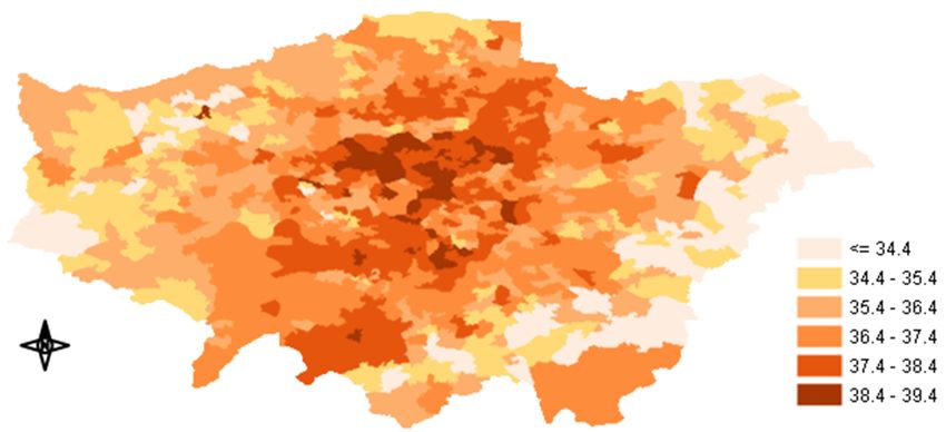
Int. J. Environ. Res. Public Health 2020, 17, x 2 of 21
Int. J. Environ. Res. Public Health 2020, 17, 1099 2 of 21
by the uncertainty of predicted population exposure. Quantifying the population exposure to air
pollution is subject to several challenges:
The spatiotemporal
The spatiotemporalvariability
variabilityofof ambient
ambient concentration
concentrationisis strongly
strongly influenced
influenced by by emissions
emissions
dynamics, predominantly from road transport, (such as peaks in traffic-related pollution
dynamics, predominantly from road transport, (such as peaks in traffic-related pollution during rush during rush
hours),meteorological
hours), meteorologicalconditions,
conditions,which
whichdetermine
determinethe thetransport
transportand anddilution
dilutionofofair
airpollutants
pollutantsandand
local conditions such as the urban form (e.g., the presence of high buildings can reduce
local conditions such as the urban form (e.g., the presence of high buildings can reduce the dispersion the dispersion
of the
of the pollutants),
pollutants),which
whichareare
thethe
most important
most factors
important leading
factors to significant
leading variationvariation
to significant of air pollutants
of air
in urban areas.
pollutants in urban areas.
Theproportion
The proportionof ofoutdoor
outdoorairairinfiltrated
infiltratedtotoindoor
indoormicroenvironments
microenvironments(MEs) (MEs)isisinfluenced
influencedby by
different housing
different housing designs
designs and
and patterns
patterns of of behaviour
behaviour inside
inside the
the building.
building.
Thespatiotemporal
The spatiotemporalvariability
variabilityof
ofpeople’s
people’sactivity
activity(population
(populationtime–activity
time–activitypatterns)
patterns)in invarious
various
MEs [4].
MEs [4].
Around75%
Around 75%of of European
Europeanpopulations
populationslive liveinincities,
cities,with
withaa highly
highly variable
variable range
range of
of activities
activities
carried out at different times and in different places [5]. The quality of data,
carried out at different times and in different places [5]. The quality of data, or the absence ofor the absence ofkey
key
components within an epidemiological exposure assessment, is likely to affect
components within an epidemiological exposure assessment, is likely to affect the magnitude and the magnitude and
significanceof
significance ofthe
theprediction
predictionmisclassification
misclassification in in aa health
health burden
burden assessment
assessment (Figure 1).
Figure 1.Figure 1. Schematic
Schematic diagramdiagram of an exposure
of an exposure assessment
assessment structurestructure forburden
for health health misclassification.
burden
misclassification.
Traditionally, epidemiological studies relied on centralized ambient concentration measurements
of limited monitoring
Traditionally, sites [6–10]. This studies
epidemiological is likely torelied
lead toon an exposure error,ambient
centralized since several monitoring
concentration
studies have suggested
measurements of limited that air pollution
monitoring data
sites from aThis
[6–10]. single site can
is likely torepresent
lead to anonly a small surrounding
exposure error, since
area especially
several monitoring in urban
studiesenvironments,
have suggested due that
to pollutants’
air pollution spatial
dataheterogeneity
from a single[11,12].
site canAmbient
representair
pollutant
only concentration
a small surrounding can be estimated
area in several
especially ways such
in urban as through due
environments, field to
observations,
pollutants’statistical
spatial
modelling such
heterogeneity as land-use
[11,12]. Ambient regression (LUR)
air pollutant and air quality
concentration candispersion
be estimatedmodels (AQM)
in several thatsuch
ways can use
as
various field
through spatial resolutions statistical
observations, [13]. Willers et al. [14]
modelling suchindicated
as land-use that regression
using air quality
(LUR) and dataair
measured
quality
at a singlemodels
dispersion site and(AQM)
assuming that that exposure
can use various across
spatialcities was the [13].
resolutions same, couldetcause
Willers considerable
al. [14] indicated
misclassification
that using air qualityof exposure.
data measuredIn their
at study,
a single they
siteexamined
and assuming the difference in mortality
that exposure risk between
across cities was the
neighborhoods
same, could cause in the city of Rotterdam
considerable and found that
misclassification the mortality
of exposure. risks between
In their neighborhoods
study, they examined thehad
a difference
difference inofmortality
up to 7%.risk By between
utilizing land use regression
neighborhoods in thetechniques and air quality
city of Rotterdam and models,
found thatseveral
the
studies have
mortality risksmanaged
betweentoneighborhoods
demonstrate that hadanaincreased
differencespatial
of up resolution of the exposure
to 7%. By utilizing land use concentration
regression
could lead to
techniques andsignificantly
air qualitydifferent
models, exposure or health
several studies haveburden
managedestimates [15–18]. Similarly,
to demonstrate that anPunger and
increased
West [19]
spatial assessedof
resolution thethe
effect of spatial
exposure resolution tocould
concentration population-weighted
lead to significantly PM2.5different
concentrations
exposurein the
or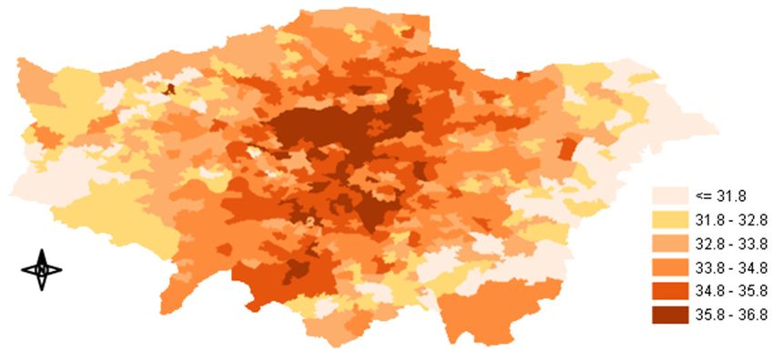
Int. J. Environ. Res. Public Health 2020, 17, 1099                                                   3 of 21

U.S. by utilizing the Community Multiscale Air Quality (CMAQ) model. They found that population
exposures, maximum concentrations and standard deviations all reduced at coarser resolutions.
At 408 km resolution, exposure and maximum concentration were 27% and 71% lower, respectively
than those at 12km resolution. Attributable mortality also reduced as the resolution became coarser.
Several studies have shown that coarse resolutions might result in lower mortality attributed to
PM2.5 [20]. Fenech et al. [21] concluded that total mortality estimates were sensitive to model resolution
up to ±5% across Europe, whereas Korhonen et al. [22] found that, considering only local sources of
primary PM2.5 , the mortality reduced by 70% in the whole country (Finland) and 74% in urban areas
when the resolution changed from 250 m to 50 km.
      Apart from the exposure misclassification due to the different levels of spatiotemporal resolution
of outdoor concentration, there are other significant contributors, in particular the infiltration of
outdoor pollutants to indoor MEs and different time-activity patterns in MEs. As particles infiltrate
and persist indoors, where people living in urban areas spent over 80% of their daily time [23], most
of the exposure to PM2.5 actually occurred in the indoor microenvironments [23–25]. The fraction
of ambient PM2.5 that infiltrates indoor microenvironments can vary due to particle size, building
characteristics, meteorological conditions and human activities [26]. Consequently, relying on outdoor
measurements alone can therefore lead to exposure misclassification. Moreover, variations in the time
spent in various MEs (e.g., outdoors, indoors, vehicles, subway) also influence population exposure
to outdoor-generated PM2.5 due to the spatial variability of both outdoor concentrations and the
indoor transport of ambient PM2.5 . Baxter et al. [27] compared four different approaches to PM2.5
exposure prediction, where each model was of a different complexity. In their study they focused
on the heterogeneity in exposures but did not investigate the influence on health effect predictions.
They suggested that geographic heterogeneity in both housing stock (and thus a relatively consistent
Air Change Rate) and human activity patterns contribute to significant heterogeneity in ambient
PM2.5 exposure both within and between cities that is not demonstrated by stationary monitors.
Ma et al. [28] compared three different types of PM2.5 exposure estimates to illustrate the differences
in exposure levels between estimates obtained from different approaches. They found that the daily
average PM2.5 exposures for residents with different activity patterns may vary significantly even
when they were living in the same neighborhood. Several studies have also investigated the correlation
between outdoor PM2.5 and mortality, although their results are skewed by the fact that people spend
the majority of the time indoors. Ji and Zhao [29] used existing epidemiological data on ambient
PM2.5 -related mortality to estimate mortality associated with indoor exposure to outdoor-generated PM.
This was the first attempt to quantify that relationship and their results indicated that outdoor PM had
substantial effects on health caused by exposure within indoor MEs. Recently, Fenech and Aquilina [30]
used the annual mean PM2.5 concentrations derived from local fixed monitoring stations to estimate
the PM2.5 -related mortality in the Maltese Islands. They found that the attributable fraction of all-cause
mortality associated with long-term PM2.5 exposure ranged from 5.9% to 11.8%, indicating that PM2.5
concentration is a major component of attributable deaths. Azimi and Stephens [31] used a modified
version of the common exposure-response function and developed a framework for estimating the
total U.S. mortality burden attributed to exposure to PM2.5 of both indoor and outdoor origins. They
found that residential exposure to outdoor-generated PM2.5 accounted for 36% to 48% of total exposure,
indicating that efforts to mitigate mortality associated with exposure to PM2.5 should consider indoor
pollution control as well.
      That of particular importance is how different exposure approaches impact long-term health
burden/mortality predictions and the magnitude of the resultant impact. We made multiple comparisons
between refined ambient PM2.5 exposure surrogates (that account for important factors such as the
infiltration and time-activity) and the fixed-site monitor PM2.5 concentrations to indicate the importance
of including more dynamic data to epidemiological studies and to demonstrate how more complex
modelling approaches modify mortality predictions. By using BenMap-CE we were able to provide the
spatial distribution of health outcomes influenced by the exposure misclassification. While a number
Int. J. Environ. Res. Public Health 2020, 17, 1099                                                                     4 of 21

of studies have already investigated exposure misclassification when using different approaches and
others have estimated health effects based on specific exposure metrics, the aim of this work is to move
one step further and answer the question: how much is the misclassification that occurs when using
different exposure approaches to predict health burden?

2. Materials and Methods
       This work aims to quantify the long-term health burden misclassification that occurs when different
PM2.5 exposure metrics are utilized. An ecologic design was used to generate associations between air
pollution exposure and health outcomes. We investigated the Greater London Area (GLA), building
on recent exposure studies that have explicitly estimated London population exposure using hybrid
dynamic models [32]. Here, we have described five different exposure Tier-models of incrementally
increased complexity are considered by gradually including data of important MEs, such as infiltration
rates of the different dwelling types and the London Underground, where London’s population spend
most or part of their daily time. The London Travel Demand Survey (LTDS) space-activity data
were categorized into three major ME groups. The analysis estimated the magnitude of the change
(i.e., avoided or incurred) in mortalities when moving from the central-site monitored concentrations as
a surrogate for population exposure (Tier-model 1) to more refined exposure Tier-models. The original
ambient PM2.5 concentrations were based on average hourly data measured by 23 monitoring stations
located in the GLA [33] and the examined MEs were: i) indoors (i.e., home-indoor), ii) aboveground
transportation iii) the London Underground and iv) outdoors. The following sections describe the
structure of the methodology and the development of each component.

2.1. Developing Tier Models to Estimate Human Exposure
     To capture different exposure assessment methods that have been used in epidemiology,
we developed five different Tier models of increased complexity, moving from static to more
dynamic approaches (Table 1). This method was separated into two parts: i) The microenvironments
and time-activity patterns were classified and calculated based on the derived information; ii) the
time-activity information was matched with corresponding microenvironmental concentrations to
estimate the dynamic time-weighted exposure. The exposure time was considered costly and the
metrics estimated the annual hourly-average PM2.5 exposures, which were then used as an input for
BenMap-CE [34].

                             Table 1. Tier models for assessing the time-weighted exposure.

  Tier Models                             Exposure Equation                                         Approach
  Tier model 1                                  E = Cout                                           Outdoors only
  Tier model 2                                  E = Cind                                            Indoor only
                                            E = Cout *Fi *xi ,
                                                P
  Tier model 3                                                                                 Indoor only (dwellings)
                        E = (Cout *tout ) +( Cout *Fi *xi )*tind + ( Cout * Fj )*       Outdoor + Indoor + Transportation
                                             P                        P
  Tier model 4
                                          tabg + (Cundg *tundg )                                  (abg. and undg.)
                       E = (Cout * tout ) + [( Cout *Fi *xi )*tind ] + ( Cout * Fj )*   Outdoor + Indoor + Transportation
                                              P                         P
  Tier model 5
                      tabg + (Cundg-hvac *tundg-hvac )+(Cdeep-undg *tdeep-undg )        (abg., deep-line + subsurface undg)

      The Tier-model stages and the respective approaches are briefly described below.
      Tier model 1: Outdoor
                                              E = Cout ,                                                                  (1)

where E is mean exposure and Cout is mean outdoor concentration of PM2.5 .
     Hourly readings were extracted from the London Air Quality Network (LAQN) [33]. LAQN
consists of automatic monitoring equipment in fixed cabins, which measures air pollution at breathing
height. It provides electronically available data on concentrations of major urban pollutants and has
been used in several studies [35,36]. The ratified concentration data from 23 available monitoring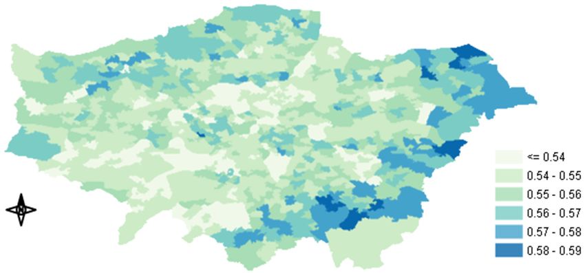
Int. J. Environ. Res. Public Health 2020, 17, 1099                                                                5 of 21

stations in GLA were downloaded and added to BenMap-CE. Only the monitors that could provide at
least 70% of the data for the whole year were selected. The ambient concentration was considered as
representative of the total population exposure.
      Tier model 2: Indoor
                                               E = Cin ,                                        (2)

where Cin is the mean indoor (i.e., home-indoor) concentration.
    This Tier model utilized the information of the spatially distributed concentration and the total
average Indoor/Outdoor (I/O) ratio in GLA to estimate the exposure inside the residence [37].
    Tier model 3: Indoor (dwellings)
                                                          X
                                                     E=        Cout * Fi * xi ,                                      (3)

where Fi is the infiltration rate of each dwelling type (i) and xi is the frequency (%) of this type
in London.
      In this study, all the indoor environments were combined into one single ME (i.e., home-indoor)
without considering other indoor environments, such as office or commercial buildings, due to the
lack of infiltration data. Subsequently, the I/O ratios that we used also represented offices and other
indoor places, assuming that the I/O ratios for other indoor MEs had the same values as domestic home
buildings [32]. The I/O ratios of London’s housing stock were obtained from Taylor et al. [37]. In their
study they estimated the Indoor/Outdoor ratio of 15 building archetypes. We grouped these archetypes
into five main dwelling types in response to available housing stock data in Middle-Super-Output-Area
resolution obtained from the Mayor of London, Datastore [38]: i) flat, ii) bungalow, iii) terraced,
iv) semi-detached and v) detached (Table 2). The frequency of each type could be calculated from the
number of properties in the GLA, which represented 98.7% of the housing (The average I/O ratio was
assigned to the unknown 1.13%). Figure 2 shows the annual average I/O ratios of PM2.5 concentration
in the GLA. The average ratios, including all dwelling types and their frequency, ranged from less
than 0.54 to 0.59. The highest ratios were observed in Outer London, whereas the lowest ratios were
observed in Inner and South West London, probably due to the newer building stock and the large
number of flats in large buildings (London Datastore), where the available surface for infiltration was
considerably smaller.

      Table 2. London’s dwelling group type descriptions, frequency in stock and average Indoor/Outdoor
      (I/O) ratios.

          Dwelling Type          Frequency %         I/O Ratios         Total Average I/O Ratio (All Dwellings)
             Bungalow                  1.81            0.63
                Flat                   50.4            0.54
              Terraced                 28.1             0.56
                                                                                         0.56
           Semi-detached               14.5            0.585
             Detached                  4.06            0.585
             Unknown                   1.13             0.56

      Tier model 4: Outdoor + Indoor + Transportation (aboveground and underground)
                                       X                         X
                 E = (Cout * tout ) + ( Cout *Fi *xi ) * tind + ( Cout * Fj ) * tabg + (Cundg * tundg ),             (4)

where (j) is each aboveground transport-ME (tMEs) and tout , tind , tabg and tundg is the fractional
time spent (%) annually outdoors, indoors, aboveground tME and London Underground (LU) tME,
respectively.
     This Tier-model includes transportation as an additional microenvironment, where an urban
population spends time during the day. This ME was categorized into aboveground and underground
transportation. Aboveground transportation refers to car, bus and train, whereas underground to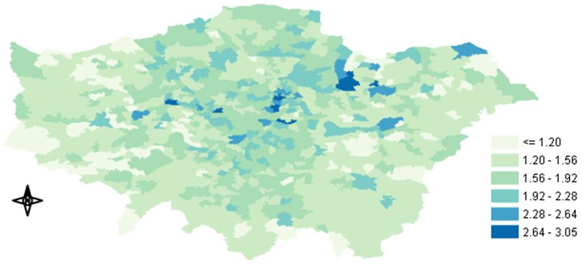
Int. J. Environ. Res. Public Health 2020, 17, 1099                                                                    6 of 21

London subway. By separating transportation into 2 groups we were able to evaluate the influence
of a highly polluted ME, like the London Underground (described in the next section), on the total
population
Int. J. Environ. exposure     concentration.
                 Res. Public Health 2020, 17, x                                            6 of 21

                   Figure 2.
                   Figure    Map of
                          2. Map of annual
                                    annual average
                                           average Indoor/Outdoor
                                                   Indoor/Outdoor (I/O)
                                                                  (I/O) ratios
                                                                        ratios used
                                                                               used in
                                                                                    in our
                                                                                       our study.
                                                                                           study.

     The
     Tier space–time–activity
          model 4: Outdoor + data Indoor for+our study were based
                                              Transportation            on the London
                                                                  (aboveground                Travel Transport Agency
                                                                                       and underground)
(LTDS) of Transport for London (TfL) [39] for the period between 2005 and 2010 (Table 3). The data
were generated fromEthe = (C out* tout) + (∑Cout*Fi *xi) * tind + (∑Cout* Fj) * tabg + (Cundg* tundg),
                           interviews     of approximately 8000 households per year, providing very useful                (4)
information  about
     where (j)      their
               is each    daily time–activity
                       aboveground                patterns,
                                          transport-ME         including
                                                           (tMEs)    and touttravel
                                                                              , tind, tmodes
                                                                                       abg and tand    trip
                                                                                                 undg is thetimes. The time
                                                                                                             fractional  data
were
spentscaled  to represent
      (%) annually         the population
                       outdoors,     indoors,ofaboveground
                                                 London, excluding        children
                                                                    tME and       London under    five years old(LU)
                                                                                             Underground           [32].tME,
respectively.
                                Table 3. Summary table of the time–activity data.
     This Tier-model includes       transportation as an additional microenvironment, where an urban
population spends       time during
               Microenvironments          the day. This Mode/Place
                                      (Groups)               ME was categorized          into
                                                                                      Time   Spentaboveground
                                                                                                     (%)           and
underground transportation. Aboveground transportation refers to car, bus and train, whereas
                                                              Walking                         1.3
underground to LondonOutdoorsubway. By separating transportation
                                                              Cycling into 2 groups we0.1     were able to evaluate
the influence Transportation
               of a highly polluted     ME, like the London Underground
                               (public/private)                 Bus               (described  0.7in the next section),
on the total population exposure concentration.                 Car                           1.6
     The space–time–activity     data   for our  study  were    Rail on the London Travel
                                                              based                           0.2 Transport Agency
                           Indoor
                                                         Underground/DLR                      0.4
(LTDS) of Transport for London (TfL) [39] for the period between 2005 and 2010 (Table 3). The data
                                                     Home, office, other indoor              95.7
were generated from the interviews of approximately 8000 households per year, providing very useful
information about their daily time–activity patterns, including travel modes and trip times. The data
wereAccording     to Smiththe
      scaled to represent    et al. [32], the of
                                population    average
                                                 London,daily  percentage
                                                          excluding          of time
                                                                      children   under spent
                                                                                          five indoors
                                                                                                years oldwas
                                                                                                           [32].95.7 %,
whereas   people   spent  2.5%,  0.4%   and  1.4%   in aboveground     transportation,      London
     According to Smith et al. [32], the average daily percentage of time spent indoors was 95.7 %,    Underground
and  outside
whereas people(walking
                   spentor  cycling),
                          2.5%,  0.4% respectively.     This proportion
                                         and 1.4% in aboveground            of time spentLondon
                                                                        transportation,      indoorsUnderground
                                                                                                        also includes
approximately   20%   of surveyed    people,  who   did not leave their  house.   In this
and outside (walking or cycling), respectively. This proportion of time spent indoors also study,  these  percentages
                                                                                                             includes
were  used  as annual    averages   for the  whole   population   over   five years
approximately 20% of surveyed people, who did not leave their house. In this study,   old,  including    the different
                                                                                                                  these
times  spent during   weekdays    and   weekends.
percentages were used as annual averages for the whole population over five years old, including
     For the in-vehicle
the different times spent exposure
                            during of    the aboveground
                                      weekdays               sub-microenvironment, we calculated the PM2.5
                                                   and weekends.
concentration by solving the mass balance equation [30]:
                                     Table 3. Summary table of the time–activity data.
                   dCin / dt = λwin * (Cout − Cin ) − ηλHVAC * Cin − Vg * (A’ / V) * Cin + Q/V,                          (5)
                  Microenvironments (Groups)            Mode/Place           Time Spent (%)
where Cout is the outdoor                                 Walking
                              concentration around the vehicle, Cin the concentration1.3 inside the vehicle,
                           Outdoor
                                                          Cycling
λwin and λHVAC are the hourly air exchange rates from the windows and mechanical     0.1 ventilation system,
               Transportation (public/private)               Bus                     0.7
respectively, n is the filter removal efficiency taking values between 0–1, Vg is the deposition velocity
                                                             Car                     1.6
in (m/h), A’ is the internal surface area, V is the volume of the vehicle and Q is the in-vehicle particle
                                                             Rail                    0.2
emission rate in µg/h. ToIndoor
                             solve this equation, the same values with Smith et al. [32] were used except
                                                      Underground/DLR                0.4
                                                  Home, office, other indoor        95.7
    For the in-vehicle exposure of the aboveground sub-microenvironment, we calculated the PM2.5
concentration by solving the mass balance equation [30]:
                          dCin / dt = λwin * (Cout – Cin) - ηλHVAC * Cin – Vg * (A’ / V) * Cin + Q/V,                    (5)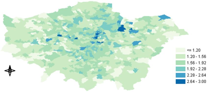
Int. J. Environ. Res. Public Health 2020, 17, 1099                                                                 7 of 21

for the concentrations and the commuter’s surface was derived from Song et al. [40], in order to
calculate A’.
     Tier model 5: Outdoor + Indoor + Transportation (aboveground and underground→ deep lines +
subsurface lines).
     The time-weighted exposure equation associated with this Tier model stage is:

           E = (Cout * tout ) + [( Cout * Fi * xi ) * tind ] + ( Cout * Fj ) * tabg + (Cundg-hvac * tundg-hvac )
                                  P                             P
                                                                                                                      (6)
                                             + (Cdeep-undg * tdeep-undg ),

     In the 5th and most complex Tier model, the same procedure as in Tier 4 was followed but the
London underground microenvironment was further divided into subsurface and deep lines to reflect
the significant difference in concentration on two types of lines. The use of mechanical ventilation in
the subsurface lines results in much lower PM2.5 concentrations than the deep lines due to air filtration
(explicitly described in the next section). Hence, by dividing the underground into two subgroups
we were able to improve the exposure estimates and to examine the contribution of a very highly
polluted microenvironment to the total exposure. The proportion of time spent in each of those two
subcategories was assumed according to the number of annual journeys completed in each line during
2017, where 77% were made by the deep-line underground and 33% by the subsurface.

PM2.5 Concentration in the London Underground
      As the London Underground microenvironment was unable to be accurately represented by
the outdoor measurements, due to its high concentration of PM2.5 and its limited connection to the
outside world, a series of air pollution measurements were conducted inside the London Underground.
The PM2.5 measurements took place on five major London Underground platforms and trains (Bakerloo
line, Circle line, Central line, District line and Victoria line) by using the portable DustTrak II Aerosol
Monitor 8534, a light scatter laser photometer, which could provide a large number of real-time
readings. The current selection of the lines was decided in order for both the deep without mechanical
ventilation lines and the subsurface with HVAC lines to be represented by our measurements.
      Our original intention was that the measurements would reflect the cold and the warm period
of 2017. Hence, the experiment was conducted during the morning and the afternoon for one week
in February and one week in July. The average concentration in the London Underground for the
whole year was very high, approximately 218 µg/m3 , albeit when we grouped the lines into deep
without HVAC lines (Central, Bakerloo and Victoria) and subsurface lines with HVAC (Circle, District)
we noticed a remarkable difference between the two concentrations (70.2 µg/m3 for the subsurface
lines and 365.6 µg/m3 for the deep lines). The PM2.5 concentration levels in the unmeasured lines
were assumed to be similar to these measured. The classification of the unmeasured lines was made
according to their depth and ventilation system.
      In the London Underground, Seaton et al. [41] reported higher platform concentrations of
480 µg/m3 . Recently, Smith et al. [42] assessed day to day variation in LU concentrations and compared
them with those above ground. During their campaign, 22 repeat journeys were made on weekday
mornings over a period of five months. They found that the subsurface ventilated District line
had the lowest PM2.5 concentration levels (i.e., mean 32 µg/m3 ) and the deep unventilated Victoria
line the highest (i.e., mean 381 µg/m3 ), while the mean concentration in the LU, according to their
measurements, was 302 µg/m3 . Although their monitoring method and equipment were different from
those used in this study and the sampling period was longer, their findings do not differ significantly
from ours. Even though the station measurements in the UK are limited, most of the studies made so
far have measured approximately two times higher concentrations in the London Underground than
in other undergrounds worldwide [43,44], probably due to its age and the limited ventilation systems.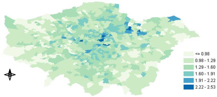
Int. J. Environ. Res. Public Health 2020, 17, 1099                                                    8 of 21

2.2. Simulating PM2.5 Exposure Concentration and Estimating Health Impact Using BenMap-CE
      The environmental Benefits Mapping and Analysis Program—Community Edition (BenMap-CE)
is a powerful Geographical Information system (GIS)-based program that estimates the health effects
associated with the change in air quality [34,45]. These data consisted of a middle layer super output
areas (MSOA) map of GLA, the derived monitoring data and London’s population data, in order to
estimate the health impact. BenMap-CE provides three interpolation methods: the closest monitor,
the fixed radius, and Voronoi Neighbour Averaging (VNA). Among the incorporated methods, VNA
was the most suitable for our case, covering the unmonitored areas and giving the best spatial
distribution of the concentration.
      After uploading the essential data and determining the appropriate Health Impact Function
(HIF) for our analysis, we were able to quantify the health impact misclassification (i.e., change in
all-cause mortality, either incurred or avoided) resulting from the exposure metric differences. In this
study, the following long-term health impact function was used to estimate the change in all-cause
mortality [46]:
                                      ∆Y = Y0 * (1 − e−β∆PM ) * Pop,                                 (7)

where ∆Y is the change in health effect, Y0 is the baseline mortality rate (the mortality rate at minimum
risk concentration), β is the unitless beta coefficient, ∆PM is the change in the exposure rates between
Tier 1 and the other Tier models (Tier 1 is the base case) and Pop is the exposed population.
      One limitation of the aforementioned effort to estimate the health impact of indoor air pollution
is the use of the mortality effect estimate (i.e., beta coefficient) that is usually taken directly from the
epidemiology literature on the studies conducted for outdoor air pollution. Therefore, to account
for that fact, some studies on the health effects of outdoor-generated PM2.5 introduced a method for
modifying the mortality effect estimate (i.e., beta coefficient) based on the average infiltration factor
combined with the mean fraction of time spent in indoor MEs [13,47,48]. However, the application
of the adjusted coefficient is solely for the component of indoor PM2.5 of outdoor origin and not
of indoor PM2.5 in total. The way indoor particle sources are treated has a larger impact than the
adjustment of the coefficient for the outdoor-generated fine particles and remains an evidence gap
of considerable public health importance. In another study, Logue et al. [49] used a central estimate
of the beta coefficient for premature mortality related to both indoor- and outdoor-generated PM2.5 ,
which was directly derived from the epidemiology literature. In our case, due to the mobile monitoring
conducted in the LU and the distinct function of BenMap-CE, a central mortality effect coefficient
from Pope et al. [50] was used as an input. The mortality effect coefficient was utilized to generate
BenMap’s health impact functions in the direction of estimating the change in estimates of mortality
(either avoided or incurred) when using different exposure metrics. Furthermore, we estimated the
percentage decrease in the predicted avoided cases when moving from the less complex (static) metrics
to more dynamic metrics.

3. Results

3.1. Exposure Metrics Summary
     The highest annual average exposure concentration was approximately 13.1 µg/m3 for Tier model
1. Tier model 2 and Tier model 3 indicated that the exposure that occurred indoors was much lower
than outdoors due to the infiltration rates of the buildings, resulting in annual average exposure
concentrations of 7.18 µg/m3 and 7.26 µg/m3 , respectively. There was an approximately 45% reduction
between Tier 1 and Tier 3. This result clearly suggests that spending long periods of time indoors,
reduces the exposure to outdoor-generated air pollution. The incorporation of transportation and
predominately the highly polluted London Underground in Tier model 4 resulted in an elevated
exposure concentration (8.28 µg/m3 ), pinpointing that even though the time spent in transit is only
2.9%, this microenvironment has a significant contribution to the total exposure. By dividing the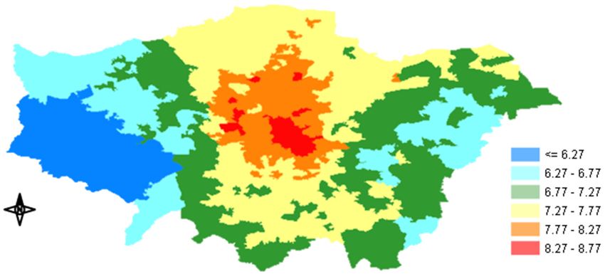
Int. J. Environ. Res. Public Health 2020, 17, 1099 9 of 21
London Underground into subsurface with HVAC and deep line without HVAC, we were able to
quantify the impact of the most highly polluted ME on the total exposures (the deep-line underground).
Tier 5 showed an approximately 0.30 µg/m3 higher exposure concentration (8.60 µg/m3 ) than Tier 4,
where an average concentration for the whole underground was used (Table 4).
Table 4. Annual exposure calculated in each model stage.
Tier Models Annual Exposure (µg/m3 ) Standard Deviation (+/– µg/m3 )
Tier model 1 13.07 1.2
Tier model 2 7.18 0.66
Tier model 3 7.26 0.66
Tier model 4 8.3 0.67
Tier model 5 8.6 0.67
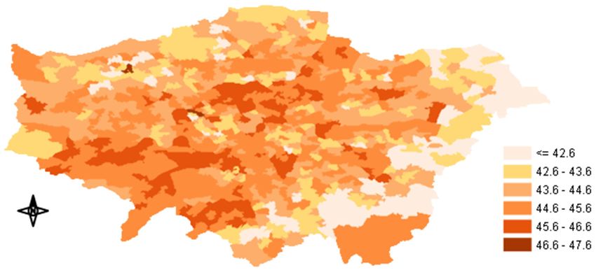
PM2.5 exposure concentration maps for each Tier-model stage were created by BenMap-CE
showing how the exposure was distributed across GLA. Figure 3a,b illustrate the spatial distribution
of the annual exposures in Tier 1 and 5. The maps of Tiers 2, 3 and 4 are included in the Supplementary
Information (Figure A1a–c in the Appendix A.1). The highest exposure concentrations occurred
in Inner London for both Tier 1 and Tier 5 (15.4 µg/m3 and 10.1 µg/m3 , respectively), whereas the
lowest exposures were observed in Western GLA (less than 10.9 and less than 7.10 µg/m3 for Tier
1 and 5, respectively). The incorporation of indoor infiltration along with time-activity data led to
an overall mitigation of the exposure concentrations in GLA when Tiers 2, 3, 4 and 5 were used. After
the utilization of our most complex model, Tier 5 had the highest difference observed at the centre
with approximately 37% (Figure 3c), while average reduction in GLA was approximately 34%. Inner
London continued to show the highest values (Figure 3b), although the infiltration factors in Inner
London were lower than in the outskirts. This could be due to the much higher outdoor concentrations
in Inner GLA than in the Outer. In Inner London, the higher number of sources of anthropogenic
and traffic-related pollutants, including PM2.5, generate significantly higher ambient pollution levels.
Several studies suggest that traffic pollutants are elevated above background concentrations around
major roads and highways [13,51]. The percentage of exposure concentration reduction in Tiers 2, 3
and 4 after comparison with our baseline exposure concentration (Tier 1), is illustrated in Figure A2a–c
in the Appendix A.2. Apart from proximity to roads, fewer green spaces and the densely constructed
city center may also contribute to the higher levels of outdoor particulate pollution [52–54]. Urban
populations are subject to daily activity patterns, so that exposure is not a static phenomenon but should
be quantified as a function of concentration and time [4]. Therefore, by assigning people’s exposure to
a single location (e.g., at their residence) and ignoring highly polluted MEs such as the subway, it is
unlikely to accurately represent total exposure. Hence, by gradually incorporating time-activity data
and indoor MEs, the spatial variability of the exposure concentration across GLA increased. Since we
used annual average time-activity data for the entire GLA, time-activity could not change the spatial
pattern of the exposure. In our case, the spatial variability of the housing stock and I/O ratios across
GLA were the main reasons for any increase in the spatial variability of the exposure concentration.
Figure 4 presents the contribution of each examined microenvironment to the total exposure
estimated by Tier-model 5. Indoor exposure concentration is clearly the dominating contributor
(approximately 83%) to the total exposure (due to the time that people spent there–95.7%) followed
by the deep-line underground ME (14%) albeit people spent on average only 0.31% of their annual
time. According to our measurements, the PM2.5 concentration in deep underground lines was around
28 times higher than the outdoor levels, which rationalized the high contribution of that ME to total
exposure. In contrast, London population spent only 1.4% of its annual time outside and the outdoor
ME contributed only 2% to the total exposure concentration. The findings described above indicate
that outdoor PM2.5 levels are unlikely to accurately represent the total exposure of an urban population
like in London.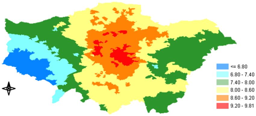
ignoring highly polluted MEs such as the subway, it is unlikely to accurately represent total exposure.
 Hence, by gradually incorporating time-activity data and indoor MEs, the spatial variability of the
 exposure concentration across GLA increased. Since we used annual average time-activity data for
 the entire GLA, time-activity could not change the spatial pattern of the exposure. In our case, the
 spatial variability of the housing stock and I/O ratios across GLA were the main reasons for any
Int. J. Environ. Res. Public Health 2020, 17, 1099                                               10 of 21
 increase in the spatial variability of the exposure concentration.

  a)

Int. J. Environ. Res. Public Health 2020, 17, x                                                                     10 of 21

  b)

   c)

       Figure      Mapsofofannual
        Figure3.3. Maps       annual  distributions
                                    distributions    across
                                                  across thethe   Greater
                                                             Greater         London
                                                                          London AreaArea  (GLA):
                                                                                      (GLA):        (a) Tier-model
                                                                                             (a) Tier-model          1
                                                                                                               1 annual
       annual mean     PM     exposure   concentration  (µg/m 3 ), (b) Tier-model 5 annual mean PM           exposure
        mean PM2.5 exposure concentration (μg/m ), (b) Tier-model 5 annual mean PM2.5 exposure
                          2.5                             3                                              2.5
       concentration          3 and (c) percentage of the PM
        concentration(µg/m
                        (μg/m),3), and (c) percentage of the PM    2.52.5exposure
                                                                          exposureconcentration
                                                                                   concentrationdifference
                                                                                                  differencebetween
                                                                                                               between
       Tier-model   1 and Tier-model
        Tier-model 1 and Tier-model 5. 5.

     Figure 4 presents the contribution of each examined microenvironment to the total exposure
estimated by Tier-model 5. Indoor exposure concentration is clearly the dominating contributor
(approximately 83%) to the total exposure (due to the time that people spent there–95.7%) followed
by the deep-line underground ME (14%) albeit people spent on average only 0.31% of their annual
time. According to our measurements, the PM2.5 concentration in deep underground lines was
around 28 times higher than the outdoor levels, which rationalized the high contribution of that ME
to total exposure. In contrast, London population spent only 1.4% of its annual time outside and the
outdoor ME contributed only 2% to the total exposure concentration. The findings described above
Int. J. Environ. Res. Public Health 2020, 17, 1099 11 of 21
Int. J. Environ. Res. Public Health 2020, 17, x 11 of 21
Figure 4. Contribution of each microenvironment (ME) to the total exposure. Indoor exposure shows
Figure 4. Contribution of each microenvironment (ME) to the total exposure. Indoor exposure shows
the greater contribution followed by the deep underground lines.
the greater contribution followed by the deep underground lines.
3.2. Epidemiological Implications and Health Impact Misclassification
3.2. Epidemiological Implications and Health Impact Misclassification
Because in epidemiology the concentration from central-site monitors is used as a proxy for the
Because
exposure in epidemiology
to air pollution, wethe concentration
selected Tier 1 asfrom central-siteand
our reference monitors
compared is used as a the
it with proxy for the
estimates
exposure to air pollution, we selected Tier 1 as our reference and compared
of Tiers 2, 3, 4 and 5. The mean change in the estimates of all-cause mortality when applying Tier it with the estimates of
Tiers 2, 3, 4 and 5. The mean change in the estimates of all-cause mortality
model 2 was predicted to be 1541 (95% CI: (427–2633)) deaths, while when using Tier 3 exposure when applying Tier model
2concentration
was predicted to be the
estimates 1541 (95%cases
death CI: were
(427–2633))
reduceddeaths,
to 1521 while
(95% CI: when
(421– using
2598)).TierThe3 impact
exposureon
concentration estimates the death
th cases were reduced to 1521 (95%
mortality when applying the 4 Tier model, which included the transportation microenvironments CI: (421– 2598)). The impact on
mortality
(tMEs), was when applying
estimated the1257
to be 4th Tier
(95% model, which included
CI: (347–2151)) cases. Duethe transportation
to the significance microenvironments
of the deep-line
(tMEs), was estimated to be 1257 (95% CI: (347–2151)) cases. Due
underground, the most complex Tier model 5 presented the lowest number of cases compared to the significance of the deep-line
with the
underground, the most complex Tier model 5 presented the lowest number
other 3 metrics (Tiers 2, 3 and 4). Namely, once Tier 5 was applied the prediction for the estimated of cases compared with
the other mortalities
avoided 3 metrics (Tiers were2,1174
3 and(95%
4). Namely,
CI: (324once Tier 5We
– 2010)). was applied
can assume thethat
prediction for the estimated
the calculated change in
avoided mortalities were 1174 (95% CI: (324 – 2010)). We can assume
mortality represents the potential health burden misclassification that might occur when changing that the calculated change in
mortality represents the potential health burden misclassification that
the exposure metrics to assess the population exposure. Subsequently, we were able to estimate might occur when changing
the
the exposure
percentage metrics to assess
decrease the population
in predicted exposure.
mortalities whenSubsequently, we were metric’s
altering the exposure able to estimate the
complexity.
percentage decrease in predicted mortalities when altering the exposure
The substantial changes in avoided mortality predictions indicate that using a static exposure approachmetric’s complexity. The
substantial changes
in a study might in to
lead avoided mortality
significant predictions
uncertainty indicate
in a health that using
burden a static exposure
assessment. approach
As anticipated, the
in a study might lead to significant uncertainty in a health burden assessment.
predicted mortality was significantly reduced when increasing the model complexity. The highest As anticipated, the
predicted
changes were mortality
observedwas in
significantly
Tier-modelreduced2 and 3,whendue to increasing
the time the thatmodel
peoplecomplexity.
spent indoors Theinhighest
urban
changes
areas, thewere observed in
big difference Tier-model
between outdoor2 andand3, indoor
due to exposure
the time thatand people spentofindoors
the absence highly in urban
polluted
areas, the big difference
transportation between outdoor
MEs, pinpointing and indoor
the importance exposure
of taking into and
seriousthe consideration
absence of highly polluted
the exposure
transportation MEs, pinpointing the importance of taking into serious
that occurs inside buildings when estimating health effects. The model predicted most avoided cases consideration the exposure
that
when occurs
Tier 2inside buildings
was applied andwhen
whileestimating
increasinghealth effects.
complexity theThe model
cases showedpredicted mostof
a decrease avoided cases
1.95%, 18.4%
when Tier 2 was applied and while increasing complexity the cases showed
and 23.8% for Tier 3, 4 and 5, respectively. As explained above, the London Underground contributes a decrease of 1.95%,
18.4% and 23.8%
significantly to thefortotal
Tieraverage
3, 4 and 5, respectively.
exposure As explained
concentration above,
of the study the London
population Underground
by increasing the
contributes
estimates. Therefore, we can securely presume that this is the main reason for the high decreaseby
significantly to the total average exposure concentration of the study population in
increasing the estimates.
avoided mortalities whenTherefore,
Tier 4 and, we can securely presume
predominantly, Tier 5 werethatused
this isinthe main reason for the high
BenMap-CE.
decrease in avoided
All results mortalities when
are summarized in TableTier5.4 and, predominantly, Tier 5 were used in BenMap-CE.
All results are summarized in Table 4.
Table 4. Change in the annual mean estimates of mortality (predicted avoided mortalities) between
the different exposure metrics and decrease between the estimated change in mortality predictions.Int. J. Environ. Res. Public Health 2020, 17, 1099 12 of 21
Table 5. Change in the annual mean estimates of mortality (predicted avoided mortalities) between the
different exposure metrics and decrease between the estimated change in mortality predictions.
Tier Models 2.5th percentile 97.5th percentile Mean Decrease (%)
Int. J. Environ. Res.
TierPublic
modelsHealth
1–22020, 17, x 427 2633 1541 12 of 21
Tier models 1–3 421 2598 1521 1.95
Tier
Tier Models
models 1–4 2.5th percentile
347 97.5th 2151
percentile Mean
1257 Decrease
18.4(%)
Tier
Tiermodels
models1–5
1–2 324
427 2010
2633 1174
1541 23.8
Tier models 1–3 421 2598 1521 1.95
Tier models 1–4 347 2151 1257 18.4
Looking at the
Tier spatial
models 1–5 distribution
324 of the predicted
2010 change 1174
in mortalities
23.8shown in Figure 5
(Tier 1–Tier 5) we
Looking canspatial
at the noticedistribution
that the biggest change inchange
of the predicted mortality occurredshown
in mortalities in central GLA.5 Several
in Figure (Tier
factors could explain this result such as the outdoor
1–Tier 5) we can notice that the biggest change in mortality PM 2.5 occurred in central GLA. Several(I/O
concentration, the housing stock ratios)
factors
and the explain
could population. As described
this result such as the above,
outdoor after
PMthe inclusion of the
2.5 concentration, the time-activity
housing stockdata there was
(I/O ratios) and an
overall reduction in
the population. Asexposure
describedconcentration
above, after the because people
inclusion usually
of the spend most
time-activity of their
data there wastimean (>95%)
overall in
indoor MEs in
reduction (excluding
exposure transportation),
concentration becausewherepeople
the concentration
usually spend of outdoor
most of PM is lower
their2.5time thaninthe
(> 95%)
measured
indoor MEsambient levels.transportation),
(excluding Because the health where impact function used
the concentration of by BenMap-CE
outdoor PM2.5 is islower
a concentration
than the
measured
response ambientthe
function, levels.
amountBecause
of thethereduced
health impact
exposurefunction used by BenMap-CE
concentration determinesis the a concentration
fraction of the
responsereduction.
mortality function, the amount
In our case,ofknowing
the reducedthatexposure
moving from concentration
Tier 1 to determines
Tier 5 would theresult
fraction
in aofgreater
the
mortality reduction. In our case, knowing that moving from Tier 1 to Tier 5
reduction of exposure concentration that appeared in central GLA (Figure 3c), we could presume that would result in a greater
thereduction of exposure
high outdoor PM2.5 concentration
concentrationthat andappeared
the buildingin central
typeGLA (Figure
of that area, 3c), welargely
were could presume
responsiblethatfor
the high outdoor PM 2.5 concentration and the building type of that area, were largely responsible for
the mortality change. The similar distribution patterns between Figures 3c and 5 also supported this
the mortality
argument. change.shown
As already The similar distribution
in Figure patterns between
2, the infiltration factorsFigure
of the 3c and Figure
buildings there5 also
were supported
lower than
this argument. As already shown in Figure 2, the infiltration factors of the
the rest of the GLA, leading to higher mitigation of the exposure concentration. In the Appendix buildings there were lowerA.3,
than the rest of the GLA, leading to higher mitigation of the exposure concentration. In the Appendix
Figure A3a–c show the spatial distribution of the predicted change in mortality between Tier 1 and
A.3, Figure A3a–c show the spatial distribution of the predicted change in mortality between Tier 1
Tiers 2, 3 and 4, respectively.
and Tiers 2, 3 and 4, respectively.
Figure5. 5. Spatial
Figure Spatial distribution
distribution ofof the
the predicted
predicted change
changeininthe
theestimates
estimatesofofmortality
mortality burden
burden
misclassification (in death cases) between Tier model 1 and Tier model
misclassification (in death cases) between Tier model 1 and Tier model 5. 5.
Overall,
Overall,these
theseoutcomes
outcomesdemonstrate the importance
demonstrate the importanceofofthethecomplexity
complexityofofanan exposure
exposure metric
metric
when incorporated into an epidemiological study. Here, we proved that indoor MEs such
when incorporated into an epidemiological study. Here, we proved that indoor MEs such as the home as the home
andand the subway are governing human exposure to air pollution and any possible absence in a metric is
the subway are governing human exposure to air pollution and any possible absence in a metric
likely to cause
is likely considerable
to cause misclassification
considerable of of
misclassification thethe
magnitude
magnitudeofofmortality.
mortality.
4. 4.
Discussion
Discussion
Due
Duetoto
the
thelimited
limitedtime
timemost
mostpeople
people spend outside, the
spend outside, theamount
amountofofambient
ambientconcentration
concentration
ofof
PM PM
2.5 2.5
that people
that areare
people directly exposed
directly to istolikely
exposed to betodifferent
is likely based
be different on variation
based in people’s
on variation behavior
in people’s and the
behavior
and the performance characteristics of the buildings they are occupying [55]. Consequently, spatial
variability, time-activity and losses due to outdoor-to-indoor transport are all sources of exposure
uncertainty in the epidemiological analysis, when fixed-site monitor concentrations are used as
surrogates for exposure to air pollution. In this work we established a more comprehensiveInt. J. Environ. Res. Public Health 2020, 17, 1099 13 of 21 performance characteristics of the buildings they are occupying [55]. Consequently, spatial variability, time-activity and losses due to outdoor-to-indoor transport are all sources of exposure uncertainty in the epidemiological analysis, when fixed-site monitor concentrations are used as surrogates for exposure to air pollution. In this work we established a more comprehensive understanding of population exposure concentration and the impact that different exposure metrics can make on all-cause mortality predictions. We showed that the I/O ratios and individual’s patterns of movement play a key role in estimating exposure to PM2.5 and that transportation-MEs, predominately the highly polluted London Underground, are important in accurately establishing exposure. We demonstrated that subway and Indoor MEs make a significant contribution to the exposure misclassification and therefore mortality change predictions. Azimi and Stephens [31] highlighted the importance of including indoor MEs when estimating the total exposure and the need for a better understanding of how the infiltration factors vary by building type in order to improve the exposure estimates and reduce the uncertainty. Based on field measurements, they found that exposure to PM2.5 of outdoor origin inside the residence contributed around 67% to the total U.S. mortality burden. In our analysis, we found that the Indoor environment contributed approximately 83% to the total mortality burden in London. The difference in our results may be explained by the different MEs considered in each study. As our aim was to quantify the misclassification and give an insight into how the absence of significant MEs from an exposure assessment could increase the uncertainty, we mainly focused on the different infiltration factors of home types and the LU. Martins et al. [56] determined the PM2.5 exposure and estimated the daily PM2.5 dose during Barcelona subway commuting. They estimated that the PM2.5 dose received by an adult in the subway contributed approximately 46% to the total daily dose in the respiratory tract. In our study, LU contributed approximately 15% to the total health burden. Due to the different methods used and different health endpoints, their results cannot directly be compared to ours. However, their outcomes indicate the non-trivial contribution from subway ME on health effects estimates. Several studies have compared static (home address-based) with more dynamic air pollution methods and proved that there is a reduction in average total exposure levels in urban areas with related characteristics as GLA [32,57]. Tang et al. [57] used a staged modelling approach to evaluate the use of static ambient concentrations as exposure estimates and examined the impact of dynamic components on estimated air pollution exposure. They found that the mean population exposures in Hong Kong for their full dynamic model were approximately 20% lower than the ambient baseline estimates of the static approach. Smith et al. [32] combined a dispersion modelling approach with building infiltration factors and travel behavior in order to create the London Hybrid Exposure Model (LHEM). They found that their model’s estimates were around 37% lower for PM2.5 than the static approach (residential address-based). Similarly, by adopting a staged modelling approach to evaluate the effect of including dynamic components to our exposure models we found that the absence of mobility and infiltration factors in the static Tier-model 1 led to an overestimation of annual PM2.5 population exposure. Overall, the exposure estimates of our most complex model (Tier 5) were around 34% lower than those of the static baseline model (Tier 1). These findings were different from Tang et al.’s [57] study but very similar to the LHEM study, mainly because the study population was the same and similar travel behavior data was used. Recently, Singh et al. [58] quantified the population exposure to PM2.5 concentrations in London and assessed the importance of including movement and indoor infiltration to total population exposure. They found that their refined exposure assessment predicted 28% lower total population exposure than the traditional static exposure method. As in this study, the time-activity data were derived from the LTDS [39] and the study area was London. However, the small difference between their results and ours could be explained by the different datasets used for the infiltration factors and the different concept used for the key MEs (e.g., the London Underground). Results from other similar studies are difficult to find as we compare different exposure estimates during the same time period (2017) in an effort to examine the effect on all-cause mortality predictions. We showed that using a static exposure metric instead of a more dynamic approach (based on time-activity data and indoor infiltration) to predict the mortality in the GLA population
You can also read