THE ENVIRONMENTAL AND ECONOMIC BENEFITS OF HIGHWAY ACCESS MANAGEMENT: A MULTIVARIATE ANALYSIS USING SYSTEM DYNAMICS
←
→
Page content transcription
If your browser does not render page correctly, please read the page content below
THE ENVIRONMENTAL AND ECONOMIC BENEFITS OF
        HIGHWAY ACCESS MANAGEMENT:
A MULTIVARIATE ANALYSIS USING SYSTEM DYNAMICS

                                    By

                              Dan Andersen

           A professional paper submitted in partial fulfillment
                       of the requirements for the

   Master of Science Degree in Environmental Policy and Management
                  Department of Environmental Studies
                  Greenspun College of Urban Affairs

                           Graduate College
                    University of Nevada, Las Vegas
                            December 2008

Abstract
         Better management of highway operations can be achieved, in part, by controlling

vehicular access to adjacent properties and cross streets. This tactic, referred to as access

management, has proven safety and operational benefits. However, doubts remain

regarding its environmental and economic benefits.

         I hypothesize that one environmental indicator, carbon emissions, will decrease with

proper access management. Controlling access increases the speed at which vehicles travel,

improving fuel efficiency and reducing carbon emissions. My hypothesis relative to

financial impacts is that access management will neither help nor harm businesses.

Controlling access can reduce travel time which has the effect of increasing the size of the

market area for businesses located on that roadway, thereby increasing their customer base.

This benefit may be off-set by the loss of some customers who are inconvenienced by

limited access.

         I used a system dynamics approach to test these hypotheses, following these five

steps: articulate the problem, formulate a dynamic hypothesis, develop a simulation model,

validate the model, and use it to evaluate policy options for addressing the problem. The

model shows that the amount of carbon emitted per vehicle mile traveled decreases 0.25%

with better access control. While this is a small amount, it equates to a 185 kg/day reduction

in carbon emissions along one sample roadway segment, and over 5,000 metric tons per

year from the entire Las Vegas Valley. The model helps us to understand how access

management impacts adjacent businesses, however the degree to which they are impacted is

inconclusive. In order to accurately model these impacts we need better data on the portion

of customers that would be deterred from visiting a business because of reduced access.

DAN ANDERSEN                                                                                     I
Table of Contents
Abstract.....................................................................................................................................i
Table of Contents ................................................................................................................ iii
Acronyms ................................................................................................................................ v
1. Introduction............................................................................................................... 1
1.1 Research Questions ...................................................................................... 1
1.2 Hypotheses.................................................................................................... 2
2. Research Method ...................................................................................................... 5
2.1 Modeling Approaches and Software Considered ................................... 5
2.1.1 Static Modeling................................................................................. 5
2.1.2 Dynamic Modeling .......................................................................... 6
2.1.3 Software for Creating System Dynamic Simulation Models ..... 8
2.2 System Dynamics Approach to Modeling Access Management........... 9
2.2.1 Problem Articulation ....................................................................... 9
2.2.2 Dynamic Hypothesis ..................................................................... 19
2.2.3 The Simulation Model ................................................................... 22
2.2.4 Model Validation ........................................................................... 32
3. Model Results and Policy Evaluation................................................................. 37
3.1 Results of Policy Tests................................................................................ 37
3.2 Results of Customer Assumptions........................................................... 40
3.3 Other Observed Results............................................................................. 42
3.4 Combined Policy Results and Evaluation............................................... 43
DAN ANDERSEN IIITABLE OF CONTENTS
4. Discussion................................................................................................................ 47
5. References................................................................................................................ 49
Tables
1 Type of Data Collected on Each Segment ........................................................................ 23
2 Arterial Segment Characteristics ....................................................................................... 24
3 Population Projections ........................................................................................................ 24
4 Carbon Emissions Formulas .............................................................................................. 26
5 Crash Rate Formulas ........................................................................................................... 27
6 Travel Speed Formulas ....................................................................................................... 28
7 Guidelines for Access Spacing (ft) on Suburban Roads (Layton 1998, TRB 2003) ..... 31
8 Output from Customer Assumptions............................................................................... 42
9 Comparative Results from the Cheyenne, Charleston, and Commerce Models........ 45
Figures
1 Reference Mode: Carbon Emissions in the Absence of Access Management ............... 3
2 Reference Mode: Decreasing Number of Customers Caused by Poor Access
Management........................................................................................................................... 4
3 Reduction in Conflict Points (TRB 2003) .......................................................................... 11
4 5-Legged Intersection.......................................................................................................... 12
5 The Compromise between Access and Mobility (TRB 2003)......................................... 14
6 Fuel Efficiency Curve (West, et. al. 1999, and DOE and EPA 2008) ............................. 16
7 Effects of Travel Time on Market Area (TRB 2003, Stover and Koepke 1988)............ 19
8 Causal Loop Diagram ......................................................................................................... 20
9 Root Model Structure.......................................................................................................... 22
10 Relationships Container Structure .................................................................................... 25
11 Carbon Emissions Relationship Diagram ........................................................................ 26
12 Crash Rate Relationship Diagram ..................................................................................... 27
13 Travel Speed Relationship Diagram ................................................................................. 28
14 Reference Mode: Carbon Emissions in the Absence of Access Management ............. 33
15 Model Output: Carbon Emissions in the Absence of Access Management ................ 33
16 Reference Mode: Number of Customers resulting from Poor Access Management . 34
17 Model Output: Number of Customers resulting from Poor Access Management .... 34
18 Market Population............................................................................................................... 35
19 Daily Traffic.......................................................................................................................... 35
20 Average Travel Speed ......................................................................................................... 36
21 Number of Driveways per Mile ........................................................................................ 36
22 Results of Driveway Spacing Policy Tests ....................................................................... 38
23 Results of Driveway Consolidation Policy Tests ............................................................ 39
24 Results of Median Installation Policy Tests ..................................................................... 41
DAN ANDERSEN IVAcronyms
AADT average annual daily traffic
CO2 carbon dioxide
DOE US Department of Energy
EPA US Environmental Protection Agency
GIS geographic information systems
HEC Hydrologic Engineering Center
MPG miles per gallon
MPH miles per hour
NCHRP National Cooperative Highway Research Program
NDOT Nevada Department of Transportation
RTC Regional Transportation Commission of Southern Nevada
TRB Transportation Research Board
TWLTL two-way left turn lanes
UNLV University of Nevada, Las Vegas
V/C volume/capacity
DAN ANDERSEN V1. Introduction
Better management of highway operations can be achieved, in part, by controlling
vehicular access to adjacent properties and cross streets. This tactic, referred to as access
management, has proven safety and operational benefits (Transportation Research Board
[TRB] 2003), however, the leading transportation research agency in the United States, the
Transportation Research Board (TRB) acknowledged that research conducted to date on the
environmental and economic impacts of access management is limited (TRB 2007). The TRB
has initiated a new research project: “Determining the Economic Value of Roadway Access
Management” (TRB 2007).
1.1 Research Questions
There are several techniques used to control access, including limiting the number of
driveways, installing raised medians, limiting the number of traffic signals, spacing traffic
signals, use of exclusive turning lanes, and implementing landuse policies that influence the
type of development adjacent to a roadway. My research focuses on the effects of the first
two techniques: limiting the number of driveways and installing raised medians. The
primary question I seek to answer through this project is how these two access management
techniques affect air quality and the financial performance of businesses that front the
roadway.
From available research we know that traffic congestion increases carbon emissions,
and we know that access management reduces traffic congestion. Therefore, we can assume
that good access management will reduce carbon emissions, but to what extent can the two
access management techniques studied here reduce carbon emissions?
DAN ANDERSEN 11. INTRODUCTION
Changing or restricting how property owners can access their property, or worse,
how customers can access businesses, is usually met with great opposition. We need to
know if access management has a negative impact on businesses. Will fewer customers visit
a store because there are fewer driveways to that store, or because there is a center median
prohibiting left-turns?
Transportation engineers and planners around the US have requested tools for
communicating the benefits of access management, needed to develop public support for
such policies (TRB 2008). Are there other benefits of access management that we can
communicate to help reduce public resistance?
1.2 Hypotheses
Relative to the effect that access management has on the environment, my
hypothesis is that uncontrolled access slows the speed at which vehicles travel, reducing
fuel efficiency and increasing carbon emissions. Therefore, controlling access by limiting the
number of driveways and installing center medians will reduce the total amount of daily
carbon emitted from vehicles using a given roadway. Without knowing exact values, I
hypothesize that carbon emissions will increase at a gradual rate in relation to traffic
congestion, as shown in Figure 1.
DAN ANDERSEN 21. INTRODUCTION
FIGURE 1
Reference Mode: Carbon Emissions in the Absence of Access Management
Carbon Dioxide Carbon Em issions w ithout Access Managem ent
08
10
12
14
16
18
20
22
24
26
28
30
20
20
20
20
20
20
20
20
20
20
20
20
Year
Relative to financial impacts to businesses, I hypothesize that limiting the number of
driveways and installing center medians may cause an initial and temporary dip in
customers, but over time will have no impact to local businesses that do not rely heavily on
drive-by traffic. Uncontrolled access slows the speed at which vehicles travel, increasing the
time it takes to travel to a particular destination on that roadway. Increased travel time has
the effect of reducing the size of the market area of the businesses located on that roadway.
Therefore, reducing the market area reduces the number of customers that will visit the
store. Figure 2 illustrates this gradual reduction in customers that may occur as a result of
poor access management. Controlling access increases the market area and market
population. A portion of customers may be lost due to the inconvenience of reduced access,
off-setting the potential increase in customers gained from increasing the market area. As
the portion of drive-by customers increases, the potential for losing them due to the
inconveniences caused by access management increases. Therefore, stores that rely on drive-
by customers will be negatively impacted by access management, while stores with a more
loyal customer base will not be negatively or positively impacted by access management.
DAN ANDERSEN 31. INTRODUCTION
FIGURE 2
Reference Mode: Decreasing Number of Customers Caused by Poor Access Management
Decreasing Num ber of Custom ers
Caused by Poor Access Managem ent
Customers
08
10
12
14
16
18
20
22
24
26
28
30
20
20
20
20
20
20
20
20
20
20
20
20
Year
DAN ANDERSEN 42. Research Method
This study follows a system dynamics approach to examine these questions. I will
first describe various modeling approaches, why I selected system dynamics, and the
software program I used. This is followed by a detailed description of the standard system
dynamics approach as I applied it to this project.
2.1 Modeling Approaches and Software Considered
There are various approaches to modeling the effects of access management.
Conceptual models—written or verbal descriptions—are used to explain theories, but lack
quantitative evidence. Physical models, such as maps and figures, can help illustrate
theories, but still lack the quantitative analysis that computer models provide. The two most
common computer models used in engineering are static and dynamic, described below.
2.1.1 Static Modeling
Models are frequently used in the field of engineering to solve complex problems—
to find the best, and sometimes only solution. The Hydrologic Engineering Center (HEC) of
the U.S. Army Corps of Engineers has developed several programs for modeling
precipitation runoff, reservoir operations, river hydraulics, sediment transport, and related
surface and groundwater hydrology (U.S. Army Corps of Engineers, 2008). Other civil
engineering models are used for modeling systems such as air dispersion, traffic patterns,
and water and wastewater distribution and treatment processes. Some are simple
spreadsheet models while others are unique software programs. Most engineers, at some
DAN ANDERSEN 52. RESEARCH METHOD
point in their education or work experience, have used models, and many use them on a
regular basis.
Some of these models are static models. Bob Diamond, president of Imagine That
Inc., a modeling software company, offers a definition of static models (2008):
“Static models describe a system mathematically, in terms of equations, where the
potential effect of each alternative is ascertained by a single computation of the equation.
The variables used in the computations are averages. The performance of the system is
determined by summing individual effects. Static models ignore time-based variances. Also,
static models do not take into account the synergy of the components of a system, where the
actions of separate elements can have a different effect on the total system than the sum of
their individual effects would indicate.”
Historically, civil engineering focused on design-related problems, whose solution
could often be derived with static models. Engineers are now called on to solve any number
of challenges, including developing management strategies and policies that guide
engineering solutions. New tools are needed to understand the complex systems that
influence policy and managerial options.
2.1.2 Dynamic Modeling
In a complex system, like highway operations, a change in one variable will cause a
change in another which ripples through the system and returns to influence the original
variable. This effect is called feedback. System dynamics describes that feedback and the
dynamic relationships, and models them to simulate the effects of implementing various
policies. Diamond provides a definition of dynamic modeling (2008):
DAN ANDERSEN 62. RESEARCH METHOD
“Dynamic modeling is a software representation of the dynamic or time-based
behavior of a system. While a static model involves a single computation of an equation,
dynamic modeling, on the other hand, is iterative. A dynamic model constantly recomputes
its equations as time changes. Dynamic modeling can predict the outcomes of possible
courses of action and can account for the effects of variances or randomness. You cannot
control the occurrence of random events. You can, however, use dynamic modeling to
predict the likelihood and the consequences of their occurring.”
The field of system dynamics was founded by Jay Forrester, aided by the advent of
computer technology that made it possible to model complex systems. In 1956, Professor
Forrester started the System Dynamics Group at the Sloan School of Management, at
Massachusetts Institute of Technology. He wrote the first book on the subject, Industrial
Dynamics, in 1961. Today system dynamics is used in a variety of disciplines, as noted by the
System Dynamics Society (2008), such as:
• “corporate planning and policy design,
• public management and policy,
• biological and medical modeling,
• energy and the environment,
• theory development in the natural and social sciences,
• dynamic decision making, and
• complex nonlinear dynamics”
DAN ANDERSEN 72. RESEARCH METHOD
2.1.3 Software for Creating System Dynamic Simulation Models
In 1985, two companies developed the next generation of computer-based system
dynamics modeling programs based on the structure of stocks and flows developed by Jay
Forrester. Ventana Systems created Vensim (Vensim 2008), and High Performance Systems
(they later changed the name to isee systems) developed Stella (isee 2008). Both have
evolved over time and are in wide use today. Powersim Software (Powersim 2008) later
introduced a similar platform which is also capable of integrating with geographic
information systems (GIS) for simulating geographical data over time.
Material and information flow into and out of stocks, where they accumulate over
time. Traditional system dynamics modeling software, such as Vensim, Stella, and
Powersim, use an icon to represent each stock. The rate at which material and information
enter and exit each stock is represented by a “flow” icon. Any number and type of variables
may influence, or be influenced by, the stocks and flows. Arrows connect the icons and
show the direction of influence. These three icons can be used to represent the structure of
any system, which makes it easy for anyone familiar with the basic concepts of system
dynamics to understand the model.
Other programs released in the past decade incorporate more graphics in an effort to
make it easier for those unfamiliar with system dynamics to understand the structure of the
model and the formulas that define it. In 1999, GoldSim introduced a graphical simulation
program that combined three types of modeling: system dynamics, discrete simulators, and
probabilistic modeling (GoldSim 2008). I developed the access management simulation
model for this project using GoldSim software. GoldSim uses many different icons, called
elements, to represent the components of the system being modeled. The system is shown
DAN ANDERSEN 82. RESEARCH METHOD
schematically and can incorporate graphics. Each element of the system can be opened to
view the formulas and relationships. This object-oriented graphical interface is helpful for
showing model logic.
2.2 System Dynamics Approach to Modeling Access
Management
The system dynamics process I followed, as described by John Sterman (2000),
involves five steps: articulate the problem, formulate a dynamic hypothesis, develop a
simulation model, validate the model, and use it to evaluate policy options for addressing
the problem.
2.2.1 Problem Articulation
More cars and trucks are using our highways than they were designed to hold,
leading to more crashes, traffic congestion, air pollution, and time spent behind the wheel.
The most common solutions to this problem are: increasing the capacity of highways,
reducing the number of vehicles on the road, and better management of highway
operations.
Increasing capacity is accomplished by building more roads or expanding the ones
we have. This helps, but is expensive, not sustainable, and environmentally damaging. The
number of vehicles on the road can be reduced by getting people to leave their cars at home
and take public transit or join a car pool. This option is the most environmentally friendly
and sustainable solution, but the least convenient. Public transit is also costly, both in terms
of the initial capital expenditure and ongoing maintenance and operations.
Better management of highway operations can be achieved, in part, by controlling
vehicular access to adjacent properties and cross streets. This tactic, referred to as access
DAN ANDERSEN 92. RESEARCH METHOD
management, is relatively effective and economical. State and local agencies are searching
for solutions to transportation problems that offer the greatest return on their investment,
especially in the face of declining tax revenues resulting from the 2008 economic slowdown.
2.2.1.1 What is Access and When is it a Problem?
Driveways and cross-streets provide drivers access to a roadway. If a driver is able
to enter or exit a driveway from any direction, that driveway has full access to the adjacent
road. Roads that have a raised center median separating opposing lanes of traffic, in front of
a driveway or at a cross-street, prevent left turns into and out of that driveway or cross-
street, and therefore limit the access at that point.
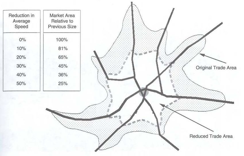
Everywhere two roads or a road and driveway meet, there are opportunities for
vehicles to collide—called conflict points. Figure 3 illustrates the number of conflict points at
a four-way intersection with and without a median. An intersection with full access has 32
conflict points, versus only 8 at an intersection with a directional median opening, which
offers some access by allowing U-turns and left turns into the cross-street. A closed median
at this intersection would only have 4 conflict points—possible rear-end collisions caused
when a vehicle makes a right-in or right-out turn.
DAN ANDERSEN 102. RESEARCH METHOD
FIGURE 3
Reduction in Conflict Points (TRB 2003)
Vehicular conflict points at a typical four-way intersection versus a directional median opening.
Even if vehicles don’t crash at a conflict point, they often have to slow down to avoid
a collision, thus slowing the flow of traffic. This slowdown creates the congestion that we all
observe, reduces fuel efficiency (US Environmental Protection Agency [EPA] 2008), and
increases emissions of greenhouse gases (Frey, et. al. 2001) which are not as immediately
discernable.
Imagine a roadway with several driveways and cross-streets in close proximity. The
conflict points at each point of access would overlap and grow significantly. To illustrate, I
was recently visiting the town of Portales, New Mexico, and observed a 5-legged
intersection surrounded by several driveways in close proximity, illustrated in Figure 4.
Standing on the northeast corner of Avenue I and 1st Street, I witnessed a northbound car on
Avenue I and a northbound car Avenue G play a game of chicken to see which could cross
1st Street first, and continue north on Avenue I. The two drivers had to be aware not only of
each other and the cross traffic on 1st Street, but of other drivers entering and exiting from
DAN ANDERSEN 112. RESEARCH METHOD
nearby driveways and cross-streets. I counted a total of 18 access points within two blocks,
and didn’t attempt to count the conflict points. This intersection has one of the highest crash
rates in Portales. Traffic volumes are not very high in Portales, so it is difficult to gauge the
effect that poor access management has on operations.
FIGURE 4
5-Legged Intersection
Within one block, 1st Street in Portales, NM, has 11 access points and an additional 7 close-by on cross-streets, shown in
red dots. The photograph was taken from the NE corner of 1st Street and Avenue I.
Avenue I
et
re
St
1 st
2.2.1.2 How is Access Managed?
Managing access involves controlling the number and spacing of driveways and
cross-streets, and the type of access provided to each. For example, a reasonable approach to
managing access at the 5-legged intersection in Portales could include closing Avenue G at
1st Street, consolidating the driveways at the parcel on the southwest corner of 1st Street and
Avenue I, and where possible, moving driveways away from the intersection. This would
reduce by a third the number of access points from this area and still provide ample access
to the church, car wash, store, laundromat, and apartment complex located at each of the
five legs of this intersection. Additional driveway consolidation would only be necessary if
crashes, volumes and congestion were very high or projected to increase significantly.
DAN ANDERSEN 122. RESEARCH METHOD
Another access management technique is the use of median treatments, including
two-way left turn lanes (TWLTL) and raised medians. Two-way left turn lanes mitigate and
reduce the effects of conflict points by removing left-turning vehicles from through traffic
lanes, therefore providing some safety and mobility benefits, however they do not reduce
the number of conflict points. Only raised medians reduce the number of conflict points.
Directional median openings typically allow left turns and U-turns to vehicles traveling on
the primary arterial, and prohibit vehicles turning left in to the arterial from a driveway or
cross-street. A fully closed median prevents all vehicles from crossing the primary arterial
and making any left turn movements.
Another technique involves the adequate spacing and timing progression of traffic
signals. Even when signals are linked together in a computerized network, it is very difficult
to time their progression when signals are too close together and not evenly spaced. Other
techniques are generally related to these and include use of exclusive turning lanes, use of
service and frontage roads, land use policies that limit right-of-way access to highways, and
separation of conflict points to reduce driver workload. My study focuses on the most
common access management techniques of installing closed medians and controlling
driveway spacing.
2.2.1.3 Balancing Access and Mobility
All of these techniques require a supporting street network to create alternate access.
A road through a residential neighborhood has a much different purpose than a freeway or
an urban arterial. Each roadway in a transportation network is assigned a functional
classification which designates the level of access it should provide and its priority within
the network. Local residential roads are allowed full access, and therefore have limited
DAN ANDERSEN 132. RESEARCH METHOD
mobility, while major highways and freeways are allowed very little access and therefore
offer greater mobility. Figure 5 illustrates the negative correlation between access and
mobility—as access decreases, mobility increases—and the types of functional classifications
associated with each. In the case of Portales’ 5-legged intersection, Avenue G is a local road,
Avenue I a collector, and 1st Street an arterial. Each serves a different purpose and should
have differing levels of access, although at present that is not the case.
FIGURE 5
The Compromise between Access and Mobility (TRB 2003)
2.2.1.4 Existing Research on the Effects of Access Management
A significant amount of research has been conducted on the effects of access
management since the 1970’s. The most comprehensive of these was conducted by the
Transportation Research Board, and published in the “Access Management Manual” which
includes a compendium of the prior research (TRB 2003). According to the TRB, access
management has an effect on safety, operations, economics, and the environment. The TRB
cites several studies to describe and quantify each of these effects. For purposes of this
DAN ANDERSEN 142. RESEARCH METHOD
study, only one methodology for quantifying the effect of each area impacted was selected
and is summarized below.
Safety
Numerous studies have shown that the crash rate increases proportionately with
access density—the number of driveways per mile. One study calculated that “crash rates
generally increase by the square root of the change in access density. Thus, an increase from
10 to 20 access points per mile would translate into about a 41% increase in the crash rate
(Levinson 2000, TRB 2003).
Roadways with continuous two-way left-turn lanes (TWLTL) are safer than
undivided roadways, while the safest roadways have nontraversable center medians. On
average, “the crash rate on roadways with a nontraversable median is about 30% less than
on those with a TWLTL” (Gluck, Levinson, Stover 1999; and TRB 2003).
Operations
Once the volume of vehicles using a roadway exceeds the free-flow capacity of that
roadway, it is congested. Congestion is measured in terms of volume/capacity (V/C). As
V/C increases, travel time on that roadway and the likelihood of vehicles crashing into each
other increases. Uncontrolled access further increases the travel time and crash rate.
Vehicles turning off of a highway must slow down to safely negotiate the turn, and as they
do so, vehicles behind them must also slow down. Numerous access points on a highway,
result in numerous opportunities for turning vehicles—slowing down the flow of traffic.
One study calculated that the overall free-flow speed is reduced by 0.15 mph per access
point (Reilly et. al. 1989 and TRB 2003).
Traffic signals also slow traffic significantly. The reduction in travel time for an
average arterial in Las Vegas, Nevada is approximately 20 seconds per traffic signal. This is
DAN ANDERSEN 152. RESEARCH METHOD
based on calculations from Las Vegas’ Regional Travel Demand Model. The formula was
modified from the Highway Capacity Manual and is based on the posted speed, signal cycle
length, green time, and signal progression on a 2-way grid (Parsons 2007).
Environment
Vehicles traveling at slower speeds, and in start and stop conditions, consume more
fuel and emit more pollutants. The operational benefits of access management, described
above, translate into better fuel efficiency and fewer emissions. Carbon emissions are
directly linked to fuel efficiency. The more fuel efficient the vehicle, the less carbon, and
other pollutants, are emitted into the environment. The US Department of Energy (DOE)
and the Environmental Protection Agency (EPA) sponsor the website
www.fueleconomy.gov to promote fuel efficient vehicles and practices. They cite a study
that states that the average vehicle achieves the greatest fuel efficiency at 60 mph (West, et.
al. 1999, and DOE and EPA 2008). At speeds slower and greater than 60 mph, vehicles
consume more fuel, as illustrated in Figure 6.
FIGURE 6
Fuel Efficiency Curve (West, et. al. 1999, and DOE and EPA 2008)
Fuel Efficiency Curve
35
30
25
Fuel Economy (mpg)
20
15
10
5
0
5 10 15 20 25 30 35 40 45 50 55 60 65 70 75
Speed (m ph)
DAN ANDERSEN 162. RESEARCH METHOD
The US EPA posts a Greenhouse Gas Equivalencies Calculator on their website
(EPA 2008) for calculating, among other things, the carbon emissions generated from
burning a gallon of gasoline—approximately 8.8 kg/gallon. Therefore, knowing the average
number of vehicles traveling a highway and the average speed at which they travel, we can
estimate the total amount of fuel consumed and carbon emitted. While not terribly accurate,
this simple method of calculating emissions is useful for comparative purposes and can be
applied to any roadway. The EPA has much more precise computer models for estimating
emissions from various vehicles, sources, and fuels under differing conditions, when those
parameters are known and available.
Economics
The economic effects of access management are the most difficult to quantify and the
most controversial. Access management is often perceived to be economically adverse to
businesses because its goal is explicitly to limit access, which most equate with limiting a
customer’s access to businesses adjacent to the roadway. Business owners want to make it as
easy as possible for customers to get to their business, by providing multiple driveways
with unrestricted access, and if possible, by installing traffic signals in front of their
business. Most feel that restricting their access will hurt their business.
On the other hand, there is anecdotal evidence that a lack of access management can
contribute to the economic decline of a business corridor. Similar to the tragedy of the
commons, a roadway is a common area available to all, but with limited capacity. For a
time, each business can have an unlimited amount of access to the highway without
adversely affecting the highway. At some point however, the highway reaches its capacity
and each additional unrestricted access point slows traffic and increases the number of
crashes. Congestion reaches a level that drivers begin to avoid the highway, when possible,
DAN ANDERSEN 172. RESEARCH METHOD
and shop at businesses located on other roadways that are safer and less congested. All
businesses along the congested roadway suffer when that occurs. To correct this, all
business must agree to share the resources of the highway by equally restricting their access.
Landscaped medians not only provide operational and safety improvements, but can
beautify a business corridor and support revitalization.
Beginning in the 1990’s, several states, most notably Kansas, Texas, Florida, and
Iowa, began studying the economic impacts of installing raised medians and consolidating
driveways (TRB 2003, Maze 1997, Eisele and Frawley 1999). These studies showed that in
implementing access management had no economic impact to most businesses. However,
businesses that rely heavily on pass-by customers, such as gasoline stations, experienced a
drop in sales after their access was restricted. In some cases, the value of adjacent properties
increased following improvements to access. These studies were primarily based on survey
results, and did not provide sufficient detail to quantify the economic impacts of access
management.
One study showed a quantifiable relationship between travel time and the size of the
market area. “Market area analysis demonstrates that increases in average travel times
translate into longer commute times and reduce the market area for businesses” (TRB 2003,
Stover and Koepke 1988). Figure 7 illustrates this effect.
DAN ANDERSEN 182. RESEARCH METHOD
FIGURE 7
Effects of Travel Time on Market Area (TRB 2003, Stover and Koepke 1988)
2.2.2 Dynamic Hypothesis
The dynamic hypothesis is developed to describe the structure of the system that is
causing the problem under consideration. This is typically accomplished with a causal loop
diagram which displays the relationships of the variables within the system. The causal loop
diagram for this study is shown in Figure 8 and described below.
DAN ANDERSEN 192. RESEARCH METHOD
FIGURE 8
Causal Loop Diagram
+
geographic size
of the market
+
number of
signals
+
number of
driveways
-
demand for
+ driveways and signals
crash rate - - +
medians
-
- + number of +
travel speed
- + businesses market
congestion + population
+
daily traffic
+ +
carbon emissions
+ + normal population
+
- +
The crash rate is influenced by the presence or absence of medians, and the
concentration of driveways and signals. Installing medians is a policy decision, and
therefore not directly influenced by other variables. There is an interesting loop affecting the
number of driveways and signals. As travel speed increases, the market area increases,
which results in an increase in the market population and therefore the number of business
along the roadway. This has the effect of increasing the demand for driveways and signals.
If the demand for driveways and signals exceeds the existing number, then more are added
DAN ANDERSEN 202. RESEARCH METHOD
which reduces the travel speed, market area and population, and puts downward pressure
on the demand for more driveways and signals. This is called a balancing feedback loop—
alternating pressures keep it somewhat balanced. Finding which has a stronger pull is
determined when these relationships are quantified.
Congestion is part of a similar balancing loop. In the absence of congestion, travel
speeds increase, increasing market area and population, and daily traffic counts. The
increased traffic increases congestion, reduces the speed, market area and population, and
eventually the daily traffic.
Carbon emissions are part of the same feedback loop with congestion, only in this
model, increased emissions don’t affect other variables. In reality, emissions could reach a
point where they influence the desirability of the area and therefore the population, but that
would likely be over a longer time period than the parameters of this model. Federal
transportation funding would be reduced if emissions exceed federal air quality standards,
but financial impacts are also outside the parameters of this model.
Customers are also part of the same feedback loop with congestion and carbon
emissions, in that they are affected by the volume of daily traffic. In addition, as access is
increased with more driveways and signals, the number of customers increases; and as
medians are installed, the number of customers decreases.
The market population will grow (or decline) according to the normal population
growth (or decline) in the area—even if the geographic size of the market remains
unchanged. A decline in the geographic size of the market, due to a decline in travel speed,
could cancel out the normal population growth in the area. Conversely, an increase in the
geographic size of the market could accelerate the normal population growth.
DAN ANDERSEN 212. RESEARCH METHOD
2.2.3 The Simulation Model
In order to test the dynamic hypothesis to see if the model reproduces the behavior I
anticipate, I developed a simulation model using GoldSim. I assigned values to each of the
variables shown in the causal loop diagram (Figure 8) and developed formulas to describe
their relationships with each other. GoldSim uses a hierarchal structure of containers and
sub-containers to organize the model. The root containers in my model include parameters,
relationships, and policies, as shown in Figure 9. The model parameters contain the values
of the data used to describe the current conditions of the roadway segment I am testing. The
relationships container houses the formulas that quantify all of the relationships among the
variables. The policies container includes policy levers used to manipulate the model, to test
various policy options. The dashboard is used to run the model, and the results container
holds graphical outputs of each model run.
FIGURE 9
Root Model Structure
Policies Relationships Parameters
DashBoard1 Results
2.2.3.1 Model Parameters
Most of the data that I used came from a study I am managing at CH2M HILL, for
the Regional Transportation Commission of Southern Nevada (RTC) (CH2M HILL 2008).
DAN ANDERSEN 222. RESEARCH METHOD
We collected data on 75 segments of arterial roadways, each approximately 7 miles in
length, throughout the Las Vegas Valley. A description of the type of data collected, and the
source for each, is shown in Table 1.
TABLE 1
Type of Data Collected on Each Segment
Characteristic Description Source
Average V/C Weighted average of V/C RTC Travel Demand Model
Average Speed Weighted average of posted speed limits RTC Travel Demand Model
Signals/Mile Total number of signals divided by the segment RTC
length
Driveways/Mile Total number of driveways divided by the segment RTC
length
Average Volume AADT averaged from NDOT traffic count locations NDOT and RTC
along the segment.
Raised Median Percent of the segment with raised median. Visual inspection using
Google Earth aerial
photographs.
Crashes/Mile Gross number of crashes from 2002 to 2006, divided UNLV, Transportation
by the segment length. Research Center
Three segments were selected for testing in the simulation model. Cheyenne Avenue
East had fairly average characteristics. Charleston Boulevard East is an older, built-out
segment with an above average number of driveways, signals, congestion, crash rate and
other characteristics. Commerce Street is less developed and has below average
characteristics. The characteristics of the selected segments, and the minimum, maximum,
and mean for the entire sampling of 75 segments are shown in Table 2. I first developed a
model using the parameters for the Cheyenne East segment. Once the Cheyenne model was
complete, I made two copies of it and changed the parameters to match those of Charleston
and Commerce.
DAN ANDERSEN 232. RESEARCH METHOD
TABLE 2
Arterial Segment Characteristics
Average Annual
Average Posted
Traveled (VMT)
Raised Median
Length (miles)
Segment with
Vehicle Miles
Speed (mph)
(5-year total)
Average V/C
Daily Traffic
Driveways
Percent of
Crashes
Signals
(AADT)
Segment
Cheyenne East 5.5 0.72 45.5 14 112 39,122 25% 2,359 216,661
Charleston East 6.8 0.76 41.9 19 273 48,900 48% 5,155 332,482
Commerce 6.4 0.49 32.8 4 63 10,070 4% 482 64,130
Min 2.2 0.07 25.9 0 15 140 0% 75 429
Max 11.9 1.17 49.7 34 428 59,763 100% 8,086 511,668
Average 7.3 0.61 38.9 13 149 25,605 38% 2,300 196,149
CH2M HILL also collected population projections in 0.5-, 1.5-, and 3-mile radii
around each segment, to the year 2030 (CH2M HILL 2008). I input this data into a 2-D table
in the model and used it to estimate population in a given year and according to the
geographic size of the market area, shown in Table 3.
TABLE 3
Population Projections
Commerce Charleston Cheyenne
0.5-mile 1.5-mile 3-mile 0.5-mile 1.5-mile 3-mile 0.5-mile 1.5-mile 3-mile
Year radius radius radius radius radius radius radius radius radius
2009 63,278 190,573 387,993 89,768 209,001 461,565 71,226 153,552 378,929
2010 67,232 199,695 406,021 91,052 212,084 469,733 72,666 157,437 390,271
2011 70,006 206,624 421,699 92,198 213,846 473,414 72,931 159,347 393,916
2012 72,780 213,552 437,377 93,344 215,607 477,095 73,195 161,256 397,561
2013 75,554 220,481 453,054 94,490 217,369 480,776 73,459 163,166 401,207
2015 81,103 234,338 484,410 96,781 220,892 488,137 73,988 166,985 408,498
2017 81,487 248,640 512,131 97,159 221,900 489,906 74,021 168,226 412,754
2020 82,062 270,093 553,713 97,725 223,411 492,559 74,070 170,088 419,138
2025 84,102 277,798 619,001 97,888 223,930 493,531 76,093 173,696 423,283
2030 85,804 283,301 654,542 99,827 228,354 503,257 77,471 176,992 431,501
DAN ANDERSEN 242. RESEARCH METHOD
2.2.3.2 Model Relationships
All of the formulas driving the model are included in the relationships container.
The sub-containers, as shown in Figure 10, help to organize the model and visually display
its structure, similar to the causal loop diagram. Each sub-container includes individual
variables, or elements, with mathematical equations describing its value in relationship to
other elements in the model.
FIGURE 10
Relationships Container Structure
+ +
-
Market_Population Market_Area Travel_Speed
-
+
+
Crash_Rate
+ Driveways Congestion
+ -
+
+
Customers
+ Daily_Traffic
+ Carbon_Emissions
The full equations and diagrams for carbon emissions, crash rate, and travel speed
are described below in detail, followed by summaries of the other sub-containers. The
carbon emissions sub-container, shown in Figure 11, includes 10 elements. The formulas
used to calculate the carbon emitted by all vehicles traveling a segment of roadway over a
given period of time are shown in Table 4. The crash rate and travel speed sub-containers
are shown in Figures 12 and 13, with the formulas used to calculate each in Tables 5 and 6.
DAN ANDERSEN 252. RESEARCH METHOD
FIGURE 11
Carbon Emissions Relationship Diagram
X
X
AADT_actual_copy
3.14
X
X X
X 16
effect_of_speed_on_mpg average_mpg daily_fuel_consumption length_copy
3.14
16 X
X
CO2_per_gallon daily_CO2_emissions
X
X X
X
CO2_per_VMT VMT_copy
TABLE 4
Carbon Emissions Formulas
Element Formula
daily_CO2_emissions daily_fuel_consumption*CO2_per_gallon
CO2_per_gallon 8.8 kg/gal (EPA 2008)
daily_fuel_consumption (length_copy/average_mpg)*AADT_actual_copy
length_copy length of the segment (a copy from the Parameters container)
AADT_actual_copy modeled average annual daily traffic (a copy from the Daily_Traffic container)
average_mpg effect_of_speed_on_mpg*average_speed_actual
average_speed_actual modeled average speed of traffic (from the Daily_Traffic container)
effect_of_speed_on_mpg look-up table based on the information illustrated in Figure 6, Fuel Efficiency Curve
CO2_per_VMT daily_CO2_emissions/VMT_copy
VMT_copy modeled vehicle miles traveled (a copy from the Daily_Traffic container)
DAN ANDERSEN 262. RESEARCH METHOD
FIGURE 12
Crash Rate Relationship Diagram
3.14 3.14 3.14
16 16 X
X 16
initial_AADT median_policy median_effect_on_crashes initial_percent_medians
3.14 B
A
C
16 X
X X
X
segment_length initial_crash_rate actual_crash_rate median_installation
3.14
16 X
X X
X
number_of_crashes driveway_effect_on_crashes driveway_increase_factor
TABLE 5
Crash Rate Formulas
Element Formula
initial_crash_rate (number_of_crashes*1,000,000)/(segment_length*5*initial_AADT*365.25 day)
initial_AADT 39,122 1/day
segment_length 5.53809625096 miles
number_of_crashes 2,359 (over a 5-year period)
actual_crash_rate initial_crash_rate*driveway_effect_on_crashes*median_installation
driveway_effect_on_crashes sqrt(driveway_increase_factor) (TRB 2003)
driveway_increase_factor driveways_per_mile_actual/driveways_per_mile_2008 (from the Driveways sub-
container)
median_installation This is a switch, or if/then/else statement, that triggers the
median_effect_on_crashes element according to the policy implementation year.
median_effect_on_crashes 1.0-0.3*(median_policy-initial_percent_medians) (TRB 2003; “The average crash
rate on roadways with a nontraversable median is about 30% less than on those
with a TWLTL.”)
median_policy User defined
initial_percent_medians 25%
DAN ANDERSEN 272. RESEARCH METHOD
FIGURE 13
Travel Speed Relationship Diagram
X
X X
X
driveways_per_mile_modeled volume_delay_function_actual
X
X X
X X
X X
X
speed_with_driveways TT_with_drive_and_signals TT_with_volume_delay average_speed_actual
3.14 3.14 3.14 3.14
X
X 16 16 16 16 X
X
cruise_speed delay_per_driveway number_signals delay_per_signal segment_length percent_change_in_speed
X
X X
X X
X X
X
speed_with_driveways_initial TT_with_drive_and_signals_ini TT_with_volume_delay_initial average_speed_initial
3.14
X
X 16 X
X
driveways_per_mile_initial initial_driveways volume_delay_function_initial
TABLE 6
Travel Speed Formulas
Elements (left to right, and Formula
top to bottom)
driveways_per_mile_modeled total_driveways/segment_length
volume_delay_function_actual 1+0.15*V_over_C_actual^4 (Bureau of Public Roads 1964)
speed_with_driveways cruise_speed-(driveways_per_mile_modeled*1 mi* delay_per_driveway)
TT_with_drive_and_signals (segment_length/speed_with_driveways)+(delay_per_signal*number_signals)
TT_with_volume_delay TT_with_drive_and_signals*volume_delay_function_actual
average_speed_actual segment_length/TT_with_volume_delay
cruise_speed speed_limit + 5 mph
delay_per_driveway 0.15 mph (TRB 2003)
number_signals 14
delay_per_signal 0.33 min (Parsons 2007; Formlua modified from Highway Capacity Manual.
Calculation is based on: 40 mph posted speed, 140 second signal cycle length with
50% green time, and signal progression on a 2-way grid.)
DAN ANDERSEN 282. RESEARCH METHOD
TABLE 6
Travel Speed Formulas
Elements (left to right, and Formula
top to bottom)
segment_length 5.53809625096 mi
percent_change_in_speed (average_speed_actual-average_speed_initial)/average_speed_initial
speed_with_driveways_initial cruise_speed-(driveways_per_mile_initial*1 mi* delay_per_driveway)
TT_with_drive_and_signals_ini (segment_length/speed_with_driveways_initial)+(delay_per_signal*number_signals)
TT_with_volume_delay_initial TT_with_drive_and_signals_ini*volume_delay_function_initial
average_speed_initial segment_length/TT_with_volume_delay_initial
driveways_per_mile_initial initial_driveways/segment_length
initial_driveways 112
volume_delay_function_initial 1+0.15*V_over_C_initial^4 (Bureau of Public Roads 1964)
The Market Population is a function of the Market Area. As the market area grows
or shrinks, it encompasses a larger or smaller portion of the population surrounding the
roadway segment. Population projections were collected from a Clark County, Nevada
geographic information system (GIS) database, in 0.5-, 1.5-, and 3-mile radii around each
segment, to the year 2030, as shown earlier in Table 3.
The Market Area assumes a starting radius of 1.5 miles around the segment. As the
as average speed at which vehicles travel through the segment decreases, due to poor
operations and congestion, the market area decreases. This is described in section 3.1.4, and
shown in Figure 8, Effects of Travel Time on Market Area.
Driveways are assumed to change in proportion to the population. This reflects the
likelihood that as the population increases in the area, their will be an increased demand for
services. More businesses will open, and as a result, more curb cuts, or driveways, will be
created.
DAN ANDERSEN 292. RESEARCH METHOD
Congestion is a simple calculation of the volume of vehicles using the segment
divided by its capacity. The capacity is assumed not to change, however volume does
change with the population.
Daily Traffic is the average annual daily traffic (AADT), which changes in
proportion with the population. In complex traffic models, AADT is a function of
population, origin and destination trips, and many other factors. To create a generic formula
applicable to any roadway segment, only population was used in this model.
Customers grow in direct proportion to the market population. Improvements in
access management increase the travel speed, which increases the market area and
population, increasing the number of customers. To date, studies have not been able to
quantify the number of customers deterred from visiting a business because of reduced
access, so assumptions are used in this model. Studies have shown that businesses that rely
on drive-by customers are impacted the most. Therefore, the model accepts user-defined
input to the current number of daily customers, the percentage of those customers that are
drive-by customers, and the percentage of total customers that are assumed to be lost as a
result of installing medians and consolidating driveways. The model outputs the number of
customers based on these assumptions. The percent of customers lost due to access
management is only the percent of drive-by customers. The model assumes that other
customers intend to visit that place of business and will find a way to gain access.
2.2.3.3 Access Management Policies
The policies tested in this model are driveway spacing and consolidation, median
installation, and the year in which these policies are implemented. The TRB published
guidelines for access spacing on principle and minor arterials, shown in Table 7 (TRB 2003).
DAN ANDERSEN 302. RESEARCH METHOD
The average arterial in the Las Vegas Valley has 20 driveways per mile, on both sides of the
road, which equates to 10 driveways per mile in each direction, for an average spacing of
528 feet. Because opposition to installing medians is far less than the opposition to
consolidating driveways, median installation will always be considered and implemented
first. For this reason, the likelihood of having a principal arterial with full median openings
(no median) is very low and the need for 2640-foot spacing not necessary. Based on this
information, the spacing options considered in this study are 330-, 660-, and 1320-feet.
TABLE 7
Guidelines for Access Spacing (ft) on Suburban Roads (Layton 1998, TRB 2003)
Functional Full Median Opening Closed Median Directional Median
Classification of Opening
Roadway (Right In/Out Only)
(left turns and U-turns)
Principal Arterial 2640 1320 1320
Minor Arterial 1320 330 660
There are two options for access spacing built in to this model. The first considers
access spacing as a policy that only applies to new development, after the policy is
implemented, and would not affect existing development. The second policy in the model
would consolidate existing driveways to meet the revised spacing requirements. In each
case, the year these policies are implemented is input into the model.
The model assumes that all medians installed will be closed, and only allow right-in
and right-out movements. The model input for this policy lever is the percent of the
segment with medians, to a maximum of 100% (openings at signalized intersections are
assumed).
The other levers relate to the customer assumptions explained at the end of section
3.3.2. These levers, or inputs, allow the user to test various customer loss assumptions. Even
DAN ANDERSEN 312. RESEARCH METHOD
the worse-case assumptions may not behave as poorly as expected, due to the positive
growth pressures that accompany good access management.
2.2.4 Model Validation
Model validation was an iterative process conducted throughout development of the
Cheyenne model—the model I later cloned to create models of Charleston and Commerce.
As each new sub-container was added to the model, the model was tested and results
checked against expected behavior. Figure 14 is a copy of the reference mode, or expected
behavior, for carbon emissions in the absence of access management. Figure 15 is the actual
model output. The trend is roughly the same.
Customer growth in the absence of access management is shown in Figure 16, the
reference mode, and Figure 17, the model output. The model output graph includes two
trend lines: actual and normal. The normal trend line assumes that customers grow directly
proportional to the projected population growth. The actual trend line assumes that
customers grow proportional to the modeled population growth, which is shrinking with
the market area as a result of poor access management. So while the modeled business is not
losing customers because of poor access management, as the reference mode suggests,
customer growth is nevertheless slower than what would otherwise have been projected.
Other selected outputs are shown in Figures 18 – 21: market population, daily traffic,
average travel speed, and the number of driveways per mile. The behavior of each matches
the expected trend.
DAN ANDERSEN 32You can also read