Global and regional climate models, sensitivity and impact experiments, response to external forcing
←
→
Page content transcription
If your browser does not render page correctly, please read the page content below
Section 7

Global and regional climate models,
sensitivity and impact experiments,
   response to external forcing
Sensitivity of Snow Water Equivalent Distribution to Variations of Critical
Snow Albedo in GCM Experiments of Hydrometcentre of Russia
Valentina M. Khan*, Konstantin Rubinstein*, Marina Zoloeva*
*- Hydrometeorological Research Center of the Russian Federation
e-mail: khan@mecom.ru
Snow is a very important component of climate system. Adequate simulation of snow cover
characteristics in hydrodynamical models is one of the indicators parameterization reliability
of hydrological and heat balance processes of the model. Simulation of snow cover area
(SCA) at global and regional scale in AMIP - type experiments was the point of special
interest in a number of publications (e.g. Frei et al. 2005). Hall & Qu, 2006, Roesch 2006
showed that snow albedo feedback is critical for climate models prediction. The objective of
the present study is to examine the effects related with introducing variable critical surface
albedo of snow in model which is in winter time directly depend on snow cover. Information
about snow density of different class of snow was obtained from Sturm, 1995 classification
approach. Then own critical value of albedo is prescribed for each class of snow cover (Tudra
– 0.95, Taiga – 0.95, Maritime – 0.7, Ephemeral – 0.5, Prairie – 0.76, Mountain – 0.87). In
the model was introduced procedure of counting dynamics of snow classes, depending on
three month mean surface air temperature, precipitation and wind. According to class of snow
cover these critical snow albedo values were introduced for experiment. For comparison, in
model control run the critical value of surface snow albedo is assumed as a constant (0.8). In
this study the SWE parameter is validated as effect of varying of snow critical albedo on the
surface.
Before evaluation process of model SWE data, we investigated which of is snow data set can
be used as etalon for evaluation of model. There is no global snow water equivalent and snow
depth datasets with good spatial and temporal resolution. Brown et al. (2003) developed
regional gridded monthly snow depth and water equivalent data set for period from 1979 to
1996 with good spatial resolution over North America region. It is not possible elaborate the
same dataset at global scale due to insufficient number of observations in situ over other parts
of the globe. In this study we verified quality of reanalysis to adequately reproduce SWE.
Validation of snow water equivalent (SWE) from 4 types of reanalysis (ERA-40 (ECMWF),
NCEP/NCAR, NCEP/DOE and JRA-25) against measured SWE from snow survey routs over
FSU territory for period from 1979 to 2000 using several statistical criteria was performed
(Khan et al., 2007). The results of comparative analysis indicated that SWE from ECMWF is
the closest to observational data for mostly FSU territory. SWE from JRA-25 reanalysis is
reasonably reproducing observational data since 1986. NCEP/DOE is only able adequately
simulate the long-term tendencies of SWE averaged over large regions. So, the global SWE
from ERA-40, ECMWF reanalysis was used for validation of outputs from GCM of
Hydrometcentre of Russia.
Both GCM experiments (control and with different albedo of classes) correspond to AMIP
protocol requirements. In the second experimental run the effect of varying surface albedo
tend to be closer to surface albedo climatologies from remote-sensed estimations.
Preliminary results indicate that seasonal variability of SWE is reproduced well in the model
for both runs, although the spatial distribution in some regions contradicts with etalon data.
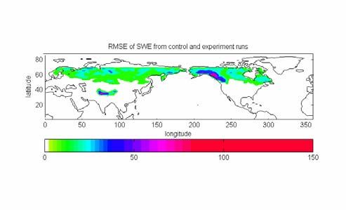
Figure 1. demonstrates seasonal distribution of SWE averaged over North America, Europe
and Asia. Results from both control and experimental runs are close to each other over large
integrated areas although they can substantially diverge at separate points. Over Europe, the
Section 07 Page 1 of 20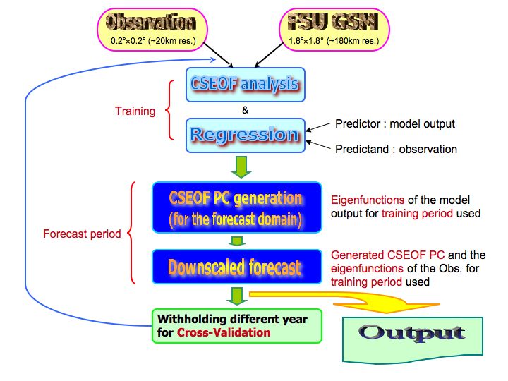
seasonal variability is reproduced well by phase, but the amplitude is underestimated by
model runs almost in twice. For Asia and North America, formation of snow cover is
simulated very close to etalon data, but the melting processes of snow are significantly
delayed. SWE from model runs overestimate SWE from ERA-40 in a range from 50%-100%.

Influence of introducing of variable critical albedo in GCM for simulation of SWE can be
seen from Figure 2. Spatial distribution of RMSE of SWE from control and experimental runs
exhibits geographical areas over globe most sensible to more accurate albedo description in
the model.

Figure1. Seasonal variability of SWE from Figure2. Spatial distribution of RMSE of
ERA-40 reanalysis, control and albedo SWE from control and experimental runs
experiments runs averaged over Europe, Asia
and North America regions
This work has been supported by the INTAS Project 03-51-5296 and NATO ESP CLG grant
981942.

References:
Brown, R. D., B. Brasnett and D. Robinson, 2003: Gridded North American Monthly Snow Depth and Snow
Water Equivalent for GCM Evaluation, Atmosphere-Ocean, 41 (1), 1–14
Frei, A., R. Brown, J.A. Miller and D.A.Robinson, 2005, Snow mass over North America: observations and
results from the second phase of the Atmospheric Model Intercomparison Project (AMIP-2), Journal of
Hydrometeorology, 6, 681-695.

Khan V.M., K.G. Rubinshtein, A.B. Shmakin, 2007, Comparison of Seasonal and Interannual Variability of
Snow Cover in Russian Watersheds According to Observations and Reanalyses , Izvestiya, Atmospheric and
Oceanic Physics, Vol. 43, No. 1, pp. 69-80

Hall, A., and X. Qu (2006), Using the current seasonal cycle to constrain snow albedo feedback in future climate
change, Geophys. Res. Lett., 33, L03502, doi:10.1029/2005GL025127.

Roesch, A., 2006, Evaluation of surface albedo and snow cover in AR4 coupled climate models, J. Geophys.
Res., 111, D15111, doi:10.1029/2005JD006473

Sturm, M., J. Holmgren, G.E. Liston, A seasonal snow cover classification system for
local to global applications, J. Climate, 8(5), 1261–1283, 1995

Section 07                                                                                            Page 2 of 20
Changes of seasonal ice area in the Arctic Ocean
                        from model simulations with IPCC SRES scenario

                              V.Ch. Khon1, I.I. Mokhov1, E. Roeckner2
             1
                 A.M. Obukhov Institute of Atmospheric Physics RAS, Moscow, Russia
                     2
                       Max-Planck Institute for Meteorology, Hamburg, Germany
                                           (khon@ifaran.ru)

     Analysis of sea ice characteristics such as a thickness and area of seasonal sea ice (or first-
year ice) area was performed using simulations with global climate model ECHAM5/MPI-
OM (Marsland et al., 2003; Roeckner et al., 2003) with the SRES A1B scenario (Houghton et
al., 2001). This scenario reaches 720ppm CO2 levels by 2100 and is one of the middle SRES
scenarios used in IPCC runs.
     Sea ice concentration and thickness were used for calculating of seasonal sea ice area.
Multiyear ice is ice that has survived at least one summer melt season (Zhang and Walsh,
2006). Consequently, we can use the summer minimum sea ice area as an indicator of
multiyear ice area. Therefore we define an area of seasonal sea ice as the difference between
the largest (April-May) sea ice area and the summer minimum (August-September) sea ice
area (Holland et al., 2006) for each year. Sea ice thickness was averaged for areas with ice
concentration more than 0.15. The Arctic region (68-90N) has been partitioned to the western
(90W; 90E) and eastern (90E; 270E) parts for the regional analysis (ACIA, 2004).
     Figure 1 shows March ice thickness (a) and the area of seasonal ice (b) as a function of the
March ice thickness for the eastern and western parts of the Arctic basin. Over the run (Figure
1), the ice cover thins from about 2 m to less than 1 m for the western Arctic and from about 4
m to less than 1.5 m for the eastern Arctic. As a result there is increasing of seasonal ice area
in the both regions. The strongest (nonlinearly as function of March ice thickness) increase of
seasonal ice has been indicated for the eastern Arctic. For the western Arctic model results
show weaker increasing of seasonal ice area with decreasing of ice thickness.

Figure 1. (a) March ice thickness and (b) the seasonal ice area as a function of the March ice thickness
for the eastern and western parts of the Arctic basin. The seasonal ice area (or open water formation
during melt season) equals the difference between the largest sea ice area and summer minimum sea
ice area for each year.

Section 07                                                                                    Page 3 of 20
This effect can be explained by changes in annual cycle of open water formation for the
selected regions of the western (Barents Sea sector) and eastern (Laptev Sea sector) Arctic.
Figure 2 shows mean area (in %) of open water in the sector of the Barents (a) and Laptev (b)
Seas for the consequent 20-years periods (2001-2020, 2021-2040, 2041-2060, 2061-2080,
2081-2100) of model simulations. For the Barents Sea model results show nearly uniform
increase of ice melting for each month. For the Laptev Sea there is strong increase of
amplitude (difference between maximum and minimum ice extent) of annual cycle due to
strong decrease of sea ice during melt season.
Figure 2. Open water area (%) in the Barents (a) and Laptev (b) Sea sectors according to model
simulations for the consequent 20-years periods (1 – [2001-2020], 2 – [2021-2040], 3 – [2041-2060], 4
– [2061-2080], 5 – [2081-2100]).
According to model results an increasing of the open water area in the Barents Sea is
connected with earlier ice melting and later ice freezing in the XXI century. For the Laptev
Sea model results show the increase for intensity of ice melting (due to strong increasing of
seasonal ice area) during warm season with a tendency to later ice freezing in the XXI
century.
This work was supported by the Russian Foundation for Basic Research and INTAS
Fellowship Grant for Young Scientists (06-1000014-6556).
References
Houghton, J. T., Y. Ding, D. J. Griggs, M. Noguer, P. J. van der Linden, X. Dai, K. Maskell,
and C. A. Johnson, Eds., 2001: Climate Change 2001: The Scientific Basis. Cambridge
University Press, 881 pp.
ACIA, 2004: Arctic Climate Impact Assessment: Scientific Report. Cambridge University
Press, 144 pp.
Marsland, S. J., H. Haak, J. H. Jungclaus, M. Latif, and F. Röske, 2003: The Max-Planck-
Institute global ocean/sea ice model with orthogonal curvilinear coordinates. Ocean Model.,
5, 91–127.
Roeckner E., Bäuml G., Bonaventura L., Brokopf R., Esch M., Giorgetta M., Hagemann S.,
Kirchner I., Kornblueh L., Manzini E., Rhodin A., Schlese U., Schulzweida U., Tompkins
A. The atmospheric general circulation model ECHAM 5. Part I: Model description / MPI
Rep. 349, Max Planck Institute for Meteorology, Hamburg. 2003.
Zhang, X., and J. E. Walsh (2006), Toward a seasonally ice-covered Arctic Ocean: Scenarios
from the IPCC AR4 model simulations, J. Clim., 19, 1730– 1747.
Holland, M. M., C. M. Bitz, and B. Tremblay (2006), Future abrupt reductions in the summer
Arctic sea ice, Geophys. Res. Lett., 33, L23503, doi:10.1029/2006GL028024.
Section 07 Page 4 of 20Impact of the North Atlantic thermohaline circulation
on the European and Northern Atlantic weather in a coupled GCM simulation
V.Ch. Khon1, M. Latif2, I.I. Mokhov1, E. Roeckner3, V. A. Semenov1,2
1
A.M. Obukhov Institute of Atmospheric Physics RAS, Moscow, Russia
2
Leibniz Institute of Marine Sciences at the University of Kiel, Germany
3
Max-Planck Institute for Meteorology, Hamburg, Germany
(khon@ifaran.ru)
Impact of the North Atlantic thermohaline
circulation (THC) on the European weather
characteristics has been analyzed using a 500-
years control simulation with the global coupled
atmosphere-ocean general circulation model
ECHAM5/MPI-OM (Marsland et al., 2003;
Roeckner et al., 2003) of spatial resolution T42
(Jungclaus et al., 2004; 2007; Pohlmann et al.,
2006). Index of North Atlantic THC was
defined as a maximum strength of ocean
meridional overturning at 30N.
Correlations between annual mean North
Atlantic THC index and precipitation, sea level
pressure (SLP), and surface air temperature
(SAT) has been computed for different seasons.
The strongest correlations are found for boreal
winter season, whilst summer season in general
does not show significant correlations. The
winter correlations are shown in the Figure 1.
As can be seen, the positive phase of the
THC is related to increase of precipitation
(decrease of SLP) over Norwegian-Barents Seas
and northern Eurasia and warming over North
Atlantic, Europe and northern Asia. These
changes are due to increased sea surface
temperatures (SST) in the Northern Atlantic
related to the positive THC phase (Latif et al.,
2004). These induce intensified advection from
the ocean to the western part of Eurasia.
Another mechanism is an increase of the
oceanic inflow to the marginal Arctic seas with
corresponding sea ice retreat. This causes
particular strong correlations in the Norwegian
and Barents Sea areas.
Changes in the SST can affect large-scale Figure 1. Correlations between low-passed
atmospheric circulation in the Northern (20-year running means) annual mean THC
Atlantic. Figure 2 shows 20-years running index and precipitation (top), sea level
mean time series of annual North Atlantic THC pressure (middle), surface air temperature
index and anomalies of wintertime Icelandic (bottom) for the winter according to model
Low intensity index in the control run. simulations. 95% significance level is +-
0.45.
Section 07 Page 5 of 20Figure 2 Time series of annual mean North Atlantic THC index and wintertime Icelandic Low (IL)
intensity index (1000mb minus SLP in the center of IL) in the control run (20-years running means).
According to the model simulation (Figure 2), there is significant modulation of the
Iceland Low intensity by the North Atlantic THC on the multidecadal timescale.
Intensification of the Iceland Low (and increase of atmospheric zonal circulation,
respectively) can produce large-scale positive anomalies in the surface air temperature over
the Eurasian continent (Figure 1, bottom).
This work was supported by the Russian Foundation for Basic Research, NATO CLG
grant 982423 (Collaborative Linkage Grant) and INTAS Fellowship Grant for Young
Scientists (06-1000014-6556).
References
Jungclaus J., Haak H., Latif M., and U. Mikolajewicz (2005), Arctic-North Atlantic
interactions and multidecadal variability of the meridional overturning circulation. J. Climate,
18, 4013-4031.
Latif, M., Roeckner, E., Botzet, M., Esch, M., Haak, H., Hagemann, S., Jungclaus, J.,
Legutke, S., Marsland, S., Mikolajewicz, U., and J. Mitchell (2004), Reconstructing,
monitoring, and predicting multidecadal-scale changes in the North Atlantic thermohaline
circulation with sea surface temperature. J. Climate, 17, 1605-1614.
Marsland, S. J., H. Haak, J. H. Jungclaus, M. Latif, and F. Rцske (2003) The Max-Planck-
Institute global ocean/sea ice model with orthogonal curvilinear coordinates. Ocean Model.,
5, 91–127.
Roeckner E., Bäuml G., Bonaventura L., Brokopf R., Esch M., Giorgetta M., Hagemann S.,
Kirchner I., Kornblueh L., Manzini E., Rhodin A., Schlese U., Schulzweida U., Tompkins A.
The atmospheric general circulation model ECHAM 5. Part I: Model description / MPI Rep.
349, Max Planck Institute for Meteorology, Hamburg. 2003.
Pohlmann H., Sienz F., and M. Latif (2006), Influence of the multidecadal Atlantic
meridional overturning circulation variability on European climate. J. Climate, 19, 6062-
6067.
Section 07 Page 6 of 20The transferability of Regional Climate Models through an assessment
of the diurnal cycle
Zavareh Kothavala1, Colin Jones1 , Dominique Paquin2 and Ayrton Zadra3
1
Centre ESCER, Université du Québec à Montréal, Canada. (Email: zav@sca.uqam.ca)
2
Ouranos Consortium, 550 Sherbrooke Street West, Montréal, Canada
3
Recherche en Prévision Numérique, Meteorological Services of Canada, Dorval, Canada
1. Introduction Site lon lat CEOP Model - Obs
Obs (K) RCA3 GEM MRCC
Three Regional Climate Models (RCMs) were imple- 1 4.93 51.97 289.94 -0.08, 1.69, -1.19
mented over seven different regions of the globe with the 2 -105.1 53.99 289.77 -1.11, 2.11, -3.17
objective of assessing their transferability to different cli- 3 106.26 45.74 291.76 -0.75, -1.10, 2.73
mate regimes. This can be explained as the ability of 4 -61.93 -10.08 299.01 4.17, 2.00, -0.93
RCMs to simulate the variability of continental scale cli- 5 147.43 -2.06 300.69 0.23, 0.19, -1.21
mates over different regions of the world with minimal pa-
rameter changes [4]. The models are: the Rossby Centre Table 1: Average July August and September 2001 2-
Regional Atmospheric Climate Model (RCA3) from Swe- meter temperature: 1. Cabauw; 2. BERMS Old Black
den [3]; the Canadian Regional Climate Model (MRCC) Spruce; 3. Mongolia; 4. Rondonia; 5. Tropical Western
[1]; and the climate version of the operational forecast Pacific (Manus). Negative anomaly values imply that the
model of Environment Canada (GEM) [2]. The RCMs model is colder than observations.
were piloted by ERA-40 and NCEP boundary conditions
for a five year period spanning from 2000 to 2004. To
fully assess the ability of the RCMs to represent the ob- is furthest from the observed at the BERMS boreal forest
served variability, field observations collected as part of the site. MRCC is closest to the observed over the tropical
Coordinated Enhanced Observation Period (CEOP) pro- rain forest and is furthest from the observed over the bo-
gram over the same period, were used as a baseline. The real Black Spruce forest. To explain these differences, an
variability of surface temperature, precipitation, humid- examination of the diurnal cycle helps yield insight into
ity, wind speed, sensible heat, latent heat, and the surface the underlying model variability.
radiation fields were examined. A succinct description of
the analysis of the diurnal cycle of precipitation and tem-
perature with three RCMs is presented for a site at a non-
native domain spanning July to September 2001.
2. Analyses
Table 1 lists the observed average temperature and
the difference from this value that was simulated by the
RCA3, GEM, and MRCC models. In order to highlight
the scope of the project, values from five sites in five dif-
ferent model domains are presented. These sites highlight
different climate regimes and a different land surface char-
acteristics. The Cabauw and Mongolia sites are grasslands
situated in maritime and continental climates respectively. Figure 1: Diurnal cycle of JAS 2001 precipitation.
The BERMS site is over the boreal forest with Old Black
Spruce vegetation. The Rondonia site covers a tropical Figure 1 shows the diurnal cycle of precipitation of the
rain forest in the Amazon. The site at Manus, is located three RCMs compared to the observations for Mongolia
on an island in the tropical western Pacific ocean. (local time = UTC + 8 hours). The precipitation accu-
For simplicity, one could regard an anomaly value close mulated over three-hour intervals were averaged over the
to ±1 K to signify that the model simulations are similar 92 days from July to September 2001. The site experi-
to the observations. By this measure, RCA3 simulates ences a dry continental climate. The CEOP observations
temperature closest to the observations for four of the five show that the time of the day with the maximum precip-
sites in Table 1. GEM simulates temperature closest to itation is at 9 hours UTC. This implies that during the
the observed at Manus in the tropical western Pacific and northern hemisphere summer, the site received most of
Section 07 Page 7 of 20the daily precipitation in the late afternoon. The three
RCMs simulate precipitation at night, unlike the observa-
tions. RCA3 simulates more than twice the total amount
of precipitation observed during this period at this site,
while GEM simulates less than half the amount observed.
Figure 2 shows the box-whisker diagrams of 3-hourly
surface temperature for the observations and the RCMs
at the same site and for the same period. The box shows
the inter-quartile range and the whiskers show the 5% and
95% values. The CEOP observations show the maximum
temperature of the day at 9 hours UTC (1700 hours local).
This corresponds to the time of maximum precipitation
in the afternoon. On the other hand, the three RCMs
show the maximum temperature at 6 hours UTC. The
excessive warm temperatures simulated by GEM causes
greater dryness due to evaporation and subsequently the
least precipitation. Interestingly, although RCA3 has an
average temperature close to the CEOP observations, the
range of temperatures is larger at all hours of the diurnal
cycle. MRCC has the coldest temperatures at 18 and 21
hours UTC i.e. the early hours of the morning at this site.
3. Summary
Only two variables at one reference site and one sea-
son are examined here due to space limitations. It should
be stressed that transferability is not an inter-comparison
exercise. The understanding of the response of RCMs to
different continental forcings have profound implications
for the hydrologic cycle and associated feedbacks, which
are vital to the study of present and future climates. The
analyses of these processes are currently being assessed.
References
[1] D. Caya and R. Laprise. A semi-implicit semi-
Lagrangian regional climate model: The Canadian
RCM. Monthly Weather Review, 127:341–362, 1999.
[2] J. Côté, S. Gravel, A. Methot, A. Patoine, M. Roch,
and A. Staniforth. The operational CMC-MRB Global
Environmental Multiscale (GEM) model. Part I: De-
sign considerations and formulation. Monthly Weather
Review, 126:1373–1395, 1998.
[3] C.G. Jones, U. Willen, A. Ullerstig, and U. Hans-
son. The Rossby Centre regional atmospheric climate
model Part 1: Model climatology and performance for
the present climate over Europe. Ambio, 33:199–210,
2004.
[4] E.S. Tackle, J. Roads, B. Rockel, W.J. Gutowski Jr,
R.W. Arritt, I. Meinke, C.G. Jones, and A. Zadra.
Transferability Intercomparison: An opportunity for
new insight on the global water cycle and energy bud-
get. Bulletin of the American Meteorological Society, Figure 2: Box-whisker diagrams of 3-hourly surface tem-
88:In Press, 2007. perature during July to September 2001 (⋆=mean).
Section 07 Page 8 of 20Sensitivity of the general circulation and extratropical cyclone characteristics to
tropical and polar heating
Eun-Pa Lim1 and Ian Simmonds2
1 Bureau of Meteorology Research Centre, GPO Box 1289K, Victoria 3001, Australia
2
School of Earth Sciences, University of Melbourne, Victoria 3010, Australia
E-mail: e.lim@bom.gov.au
In a warmer globe caused by increasing CO2 greater warming is expected over the polar region in the
lower troposphere and over the tropics in the upper troposphere (Figure 1) (IPCC 2001), and
Southern Hemisphere winter extratropical cyclones in the CSIRO Mark2 atmosphere-ocean coupled
model are seen to reduce in their number with doubled CO2 (Figure 2) (Sinclair and Watterson 1999,
Lim 2005). In this study we examine the influence of each of the tropical and the polar warming on
the general circulation and the characteristics of Southern Hemisphere (SH) extratropical low
pressure systems by conducting idealised temperature 'nudging' experiments.
Using Melbourne University atmospheric general circulation model (MUGCM, R21/L9),
warm temperature anomaly, 0.04ºC hr-1 was nudged over (a) the tropics between 21.5ºS and 21.5ºN at
sigma level = 0.336 - TU (Tropics/Upper level); (b) the high latitudes between 65ºand 90º latitudes in
both hemispheres at sigma = 0.991 and 0.926 - HL (High latitude/Lower level); and (c) the tropics at
sigma = 0.336 and the high latitudes at sigma = 0.991 and 0.926 - TU+HL. These warm anomalies
were forced at all points on the relevant latitude circles. The resultant vertical temperature profile is
shown in Figure 3.
Our three sets of 8 year MUGCM simulations demonstrate that warming over the tropics in
the upper troposphere results in stronger Ferrel circulation and westerlies between 40ºS and 60ºS in
winter. Whereas, warming over the high latitudes in the lower troposphere causes the meridional and
vertical circulations to be slightly weaker over most of the SH extratropics and the upper level zonal
winds to be less strong over the 60ºS latitude band. When the equal amount of positive temperature
anomaly was nudged over the high latitudes in the lower troposphere and over the tropics in the
upper troposphere, the weakening of the meridional-vertical circulation is more obvious than that in
the HL experiment. The axis of westerly jet tends to move equatorward.
Figure 4 shows zonal means of winter MSLP cyclone system density and depth which were
simulated in three different nudging experiments. Warming in the TU experiment tends to cause the
frequency and depth of extratropical cyclones to increase in the high latitudes at the surface. By
contrast, warming over the high latitudes in the lower troposphere (HL and TU+HL), the frequency
and depth of MSLP cyclones tend to decrease in the higher latitudes. In the midlatitudes between
30º-50ºS fewer surface cyclones are found with the TU warming, but slightly more systems are found
with the HL and TU+HL warming. However, the cyclone property changes with the HL and TU+HL
warmings are very subtle in the midlatitudes, and it needs further investigation whether this less
sensitivity to the polar warming is model dependent or not.
Consequently, the TU warming seems an important contributor to the decrease in cyclone
system density over most of the SH extratropics in a doubled CO2 atmosphere shown in Figure 2.
IPCC (2001). Climate Change 2001, The scientific basis, edited by Houghton, J.
T., Y. Ding, D. J. Griggs, M. Noguer, P. J. van der Linden, X.Dai, K. Maskell
and C. A. Johnson. Cambridge, U.K.: New York, USA: Cambridge University Press.
Lim, E.-P. (2005). Global changes in synoptic activity with increasing atmospheric CO2, Ph. D.
thesis, University of Melbourne, Victoria, Australia
Sinclair, M. R. and I. G. Watterson (1999). Objective assessment of extratropical weather systems in
simulated climates, Journal of Climate, 12, 3467-3485.
Section 07 Page 9 of 20Figure 1 Vertical profile of annual mean temperature Figure 2 Changes in MSLP cyclone system
change of 2xCO2-1xCO2 simulated in the CSIRO Mk2 density from 1xCO2 to 2xCO2 simulated in
AOGCM. The contour interval is 0.5 K. the CSIRO Mk2 AOGCM. Shaded areas
show
positive changes, and stiples show
statistically
significant changes at the 95% confidence
level
(a) (b) (c)
Figure 3 Vertical profile of annually averaged temperature difference between the control experiment and
(a) the tropical/upper troposphere (TU) warming, (b) the high latitudes/lower troposphere (HL) warming,
and (c) the TU+HL warming experiments. The arrows indicate the locations where the temperature forcing
is placed. The contour interval is 0.5 K.
(a) (b)
Figure 4 Zonal means of MSLP cyclone (a) system density and (b) depth simulated in the control run
(solid line) and the transient runs with the TU warming (solid long dash line), the HL warming (solid short
dash line), and the TU+HL warming (short dash line)
Section 07 Page 10 of 20Categorical predictability of regionalized surface temperature and
precipitation over the southeast United States
Young-Kwon Lim, D. W. Shin, T. E. LaRow, and S. Cocke
Center for Ocean-Atmospheric Prediction Studies, Florida State University, Tallahassee, FL 32306-2840
(lim@coaps.fsu.edu)
Coarsely resolved surface temperature and precipitation which are seasonally integrated
using the FSU/COAPS GSM (Florida State University/Center for Ocean-Atmospheric Prediction
Studies Global Spectral Model, ~1.8° lon.-lat. (T63)) for the period of 1994 to 2002 (March
through September each year) are downscaled to local spatial scale of ~20 km for the southeast
United States (Florida, Georgia, and Alabama) by applying both dynamical and statistical
methods. This study is performed since 1) the individual local areas over the southeast United
States frequently face extremely high temperature and the heavy rainfall with severe storms
during summer, resulting in the devastating property damage and injuries. An accurate seasonal
forecast with higher spatial resolution is essential to mitigate damage in advance. 2) This region is
also noted for some of the largest areas of agricultural farms in the nation. Various kinds of crops
and fruits (e.g., peach, tomato, corn, tangerine, peanut, citrus, and strawberry) are raised in these
regions. Farmers and agricultural researchers need accurate climate forecasting to adapt
management, increase profits, and reduce production risks.
Dynamical downscaling is conducted by running the FSU/COAPS Nested Regional
Spectral Model (NRSM), which is nested into the domain of the FSU/COAPS GSM (GSM) (Shin
et al. 2006; Cocke et al. 2007). A statistical downscaling is newly developed in this study. The
rationale for this approach is that clearer separation of prominent local climate signals (e.g.,
seasonal cycle, dominant intraseasonal or interannual oscillations) in the observations and the
GSM over the training period can facilitate the identification of the statistical relationship
associated with climate variability between two datasets, which eventually leads to better
prediction of local climate scenario from the large-scale simulations. The techniques primarily
applied for statistical downscaling are Cyclostationary EOF (CSEOF) [Kim and North, 1997],
multiple regressions, stochastic time series generation, and the cross-validation. Overall
downscaling procedures are illustrated by the schematic diagram in Fig. 1.
Downscaled data are compared with the FSU/COAPS GSM fields and observations.
Downscaled seasonal anomalies reasonably produce the local surface temperature and
precipitation scenario from the coarsely resolved large-scale simulations. A series of evaluations
including correlations, frequency of extreme events, and categorical predictability demonstrate
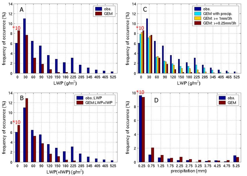
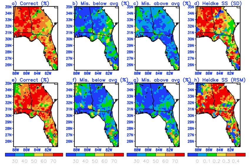
the reliability of these downscaling models. As shown in Fig. 2 and 3 as examples, categorical
predictability for seasonal maximum temperature anomaly (Tmax) and rainy/dry periods reveals
the correctness in percentage prevailing from 60 to 80 (Tmax) and, from 50 to 70 (precipitation) by
both downscaling methods, supporting that our downscalings yield the predictability perceptibly
greater than random chance. The skill of this local forecast is comparable to or greater than
predictability of large-scale NCEP climate seasonal forecasts [Saha et al., 2006]. Much lower
incorrectness in percentage shown on the second and third column of figures, and the Heidke skill
scores on the fourth column demonstrate the reliable skill of these downscaling approaches.
Although there still remains a room for the improvement in predictive skill, these downscaled
model results are reliable and can be used in many application models (e.g., crop model).
Acknowledgement
COAPS receives its base support from the Applied Research Center, funded by NOAA Office of Global
Programs awarded to Dr. James J. O’Brien.
Section 07 Page 11 of 20Figure 2. Categorical predictability in percentage
(the left three columns) and Heidke Skill Score
(right column) for the downscaled seasonal Tmax
anomaly. Two classes from categorization are 1)
above climatological Tmax and 2) below
climatological Tmax. Top panel depicts the result
from the statistical downscaling whereas bottom
Figure 1. Schematic diagram of statistical panel the dynamical downscaling (the NRSM).
downscaling procedure in the present study. The first three columns from the left illustrate the
Downscaling has been conducted using percentage of 1) correct prediction (the sign of
Cyclostationary EOF, multiple regression, and the downscaled anomaly & observed anomaly is
time series generation techniques. Downscaled data Pab
are produced over 9 years (1994-2002) by same), 2) ! 100 (see the schematic
repeatedly withholding a particular year and placing Paa + Pab
it on the prediction period under the cross-validation Pba
framwork. probability table below), and 3) ! 100
Pba + Pbb
(see table below).
Downscaled Forecast Downscaled Forecast
Verifying analysis
Verifying analysis
above below above below
average average
Obs. Above Paa Pba
average
PaP
avera
Obs. Below PabAbove Pbb Pb P P
aa Pba
Below Pab Pbb
PaF PbF 1
PaF PbF
Downscaled Forecast
Verifying analysis
wet period dry period
Obs. wet period Paa Pba PaP
Figure 3. Same as Fig. 2 but for rainfall periods. dry period Pab Pbb PbP
The 5-day interval during which precipitation
amount is greater than 5mm is classified into wet PaF PbF 1
period otherwise the dry period (see table right).
References
Cocke, S., T. E. LaRow, and D. W. Shin, 2007: Seasonal rainfall prediction over the southeast U.S. using
the FSU nested regional spectral model. J. Geophys. Res., 112, D4, D04106, doi:10.1029/2006JD007535.
Saha, S., and Coauthors, 2006: The NCEP climate forecast system. J. Climate, 19, 3483-3517.
Shin, D. W., J. G. Bellow, T. E. LaRow, S. Cocke, and J. J. O’Brien, 2006: The role of an advanced land
model in seasonal dynamical downscaling for crop model application. J. Appl. Meteor. Climatol., 45, 686-
701.
Section 07 Page 12 of 20The Simulated Surface Radiation Budget over North America
in a Suite of Regional Climate Models
Marko Markovic 1 , Colin Jones 1 , Paul Vaillancourt 2 , Dominique Paquin 3
1
University of Quebec at Montreal, 2Environment Canada, 3Consortium Ouranos
markovic@sca.uqam.ca
Downward longwave €radiation (DLR) € and shortwave€radiation (ISR) are€important parameters in
climate models, being the main terms in the surface energy balance controlling the evolution of surface
temperature and soil moisture. Systematic biases in the representation of surface radiation can lead to
errors in a number of key near surface climate variables (e.g. soil moisture, snow cover and sea-ice). In
this report we evaluate the DLR and ISR simulated by 3 Regional Climate Models (RCMs) over North
America. The RCMs used are: The Canadian Regional Climate Model (CRCM, version 4.0.2) (Caya
and Laprise 1999), GEM-LAM, the regional version of the Global Environmental Multiscale Model
(Côté et al 1998) and the Swedish Rossby Centre Regional Climate Model, RCA3, (Jones et al. 2004).
Observations are derived from six measurement sites within the NOAA-SURFRAD (Surface Radiation
Budget) network, representing a cross-section of various climate types over North America. 3-hourly,
grid point DLR and ISR values, collocated with the 6 SURFRAD sites, were extracted from the
respective RCM simulations and form the basis for an evaluation of the simulated surface radiation.
Figure 1 presents a normalized frequency distribution (FD) of surface ISR and DLR separately for
summer (JJA) and winter (DJF) from the 3 models and surface observations. The FDs are averaged over
the 6 observation sites. Cloud free conditions are defined as a given 3-hour period having a cloud cover
less than 10% in both observations and model, while cloudy conditions are when each data set has a
cloud cover value greater than 90%. All sky is the total surface radiation for all cloud cover conditions.
The DJF distribution of all-sky DLR (Fig. 1d) shows all models biased towards low values. For RCA3
and GEM-LAM this is due to a negative bias in the clear-sky DLR frequency distribution (Fig. 1e),
cloudy-sky DJF DLR (Fig. 1f) being well simulated by these 2 models. A negative bias in simulated
clear sky DLR in cold, dry winter conditions was also seen by Wild et al. (2000). This problem is often
due to inaccuracies in either the representation of the water vapor continuum in dry conditions or
deficiencies in including the contribution of trace gases and aerosols to the total DLR. CRCM has the
same DLR clear-sky error (Fig. 1e) but also a negative bias in DJF DLR under cloudy skies (Fig. 1f).
GEM-LAM and CRCM represent the distribution of all-sky DJF ISR well (Fig. 1a). Clear sky ISR DJF
(Fig. 1b) is accurate in both models, while GEM shows the best result in cloudy conditions (Fig. 1c).
The cloudy-sky DJF ISR is biased low in CRCM, suggesting winter clouds are optically too thick with
respect to solar radiation. This is in contrast to the DJF DLR cloudy-sky errors in CRCM, biased
towards low values, which is consistent with too low cloud emissivity. Cloud water appears to be treated
in an inconsistent manner between the 2 radiation streams in CRCM. The negative bias in CRCM DJF
cloudy-sky ISR (Fig. 1c) is balanced by an overestimate of the occurrence of clear-sky conditions
(underestimated cloud cover, not shown). RCA3 DJF all sky ISR (Fig. 1a) has too few occurrences of
low ISR (< 200Wm-2) and too many occurrences in the range 200-600Wm-2. RCA3 simulated clouds in
DJF appear to contain too little water or have a systematic underestimate in the effective radius leading
to winter clouds that have too low albedo. Clear sky DJF ISR (Fig. 1b) is quite accurate in RCA3.
In JJA CRCM has a bias towards low values of all-sky DLR (Fig.1j), due to an underestimate of cloudy-
sky DLR (Fig. 1l), also consistent with an underestimate of cloud emissivity. The negative bias in
cloudy-sky DLR in CRCM during JJA is partially balanced by a positive bias in clear-sky DLR. This
arises either from the CRCM atmosphere being too warm, and/or clear-sky conditions in CRCM, at high
Section 07 Page 13 of 20water vapor concentrations, being frequently simulated as cloud-free while the same moisture conditions
produce a cloud in observations (CRCM systematically underestimates JJA cloud cover, not shown).
GEM-LAM has a similar bias to CRCM in clear sky JJA DLR (Fig. 1k), probably for similar reasons.
RCA3 gives an accurate JJA ISR all-sky distribution (Fig. 1g) while both GEM-LAM and CRCM
overestimate the occurrence of high ISR values. RCA3 is biased towards too many occurrences of very
low ISR (440Wm-2) in RCA3 in JJA(Fig. 1l). All 3 models underestimate cloud fraction
in the JJA, we therefore conclude that the accurate total sky ISR (Fig. 1g) in RCA3 results from an
overestimate of clear-sky radiation, due to an overestimate of clear-sky occurrence, balanced by clouds
that are too reflective when present. GEM-LAM has numerous occurrences of very high cloudy-sky ISR
in JJA (>800Wm-2) (Fig. 1i). These cloudy-sky ISR values only occur for optically thin cirrus,
suggesting an overestimate of these cloud types in GEM-LAM. The JJA ISR bias in CRCM seems
mainly due to clear sky errors (e.g. the clear sky is too transmissive).
Figure 1: Distribution of ISR and DLR
3-hourly radiation fluxes from RCMs
and observations. The period 15-21
UTC is analysed due to cloud
observations only being available
during sunlight: a) winter ISR all sky,
b) winter ISR cloud free, c) winter ISR
cloudy, d) winter DLR all sky, e) winter
DLR cloud free, f) winter DLR cloudy,
g) summer ISR all sky, h) summer ISR
cloud free, i) summer ISR cloudy, j)
summer DLR all sky, k) summer DLR
cloud free, l) summer DLR cloudy.
References:
Caya D and Laprise R. 1999: A Semi-Implicit Semi-Lagrangian Regional Climate Model: The Canadian RCM. Monthly
Weather Review, 127: 341-362.
Jones, C. G., Willén, U., Ullerstig, A. and Hansson, U 2004: The Rossby Centre Regional Atmospheric Climate Model Part I:
Model Climatology and Performance for the Present Climate over Europe. Ambio 33:4-5, 199-210., 2004
Cote, J., S. Gravel, A.Methot, A. Patoine, M. Roch, and A. Staniforth 1998: The operational CMC-MRB global
environmental multiscale (GEM) model. Part I: Design considerations and formulation. Mon. Wea. Rev, 126, 1373-1395.
Wild et al. Evaluation of Downward Longwave Radiation in General Circulation Models, Journal of Climate, 2000
Section 07 Page 14 of 20Comparison of cloudiness and cyclonic activity changes over extratropical latitudes in
Northern Hemisphere from model simulations and from satellite and reanalysis data
I.I. Mokhov1, M.G. Akperov1, A.V. Chernokulsky1, J.-L. Dufresne2, H. Le Treut2
1
Obukhov Institute of Atmospheric Physics RAS, Moscow, Russia
2
Laboratoire Meteorologie Dynamique du CNRS, Paris, France
mokhov@ifaran.ru
Changes of cloudiness and cyclonic activity over extratropical latitudes in the
Northern Hemisphere (NH) from simulations with the coupled general circulation model
(CGCM) are analyzed in comparison with satellite and reanalysis data.
Results of the IPSL-CM4 (version 1) CGCM (Marti et al., 2005) simulations for 1860-
2000 with the greenhouse gases concentrations in the atmosphere from observations and for
2001-2100 with the SRES-A2 scenario are used.
Model results are compared to the cyclonic activity characteristics (Bardin and
Polonsky, 2005; Golitsyn et al., 2006; Golitsyn et al., 2007) on the basis of NCEP/NCAR
reanalysis data (Kistler et al., 2001) during 1952-2000 and to the satellite cloudiness data
(Rossow and Duenas, 2004) for 1983-2000.
Daily data for cyclonic characteristics from model simulations were obtained similar
to (Bardin and Polonsky, 2005; Golitsyn et al., 2006; Golitsyn et al., 2007). Here we analyze,
in particular, the part of total area covered by cyclones or density of cyclones packing (DCP)
defined similar to (Mokhov et al., 1992).
Figure 1 shows changes of total cloudiness and DCP over extratropical latitudes (20-
o
80 N) from model simulations for periods 1860-2000 (a) and 2001-2100 (b). Values on Fig.1
were normalized on their mean values for the period 1961-1990. Figure 1a does not show
significant changes in total cloudiness and DCP while Fig.1b shows tendency of decrease for
both variables in the 21st century. This tendency is related to a general tendency of decrease in
the temperature difference between high and low latitudes with a general decrease of
tropospheric baroclinic instability under global warming (Mokhov et al., 1992).
Analysis of relationship between total cloudiness by satellite monthly data and DCP
by reanalysis monthly data for the NH extratopics shows significant positive correlation for
the period 1983-2000 while no correlation was found by annual-mean data. Model
simulations do not exhibit significant correlation for this period both by monthly-mean and
annual-mean data but display positive correlation for longer periods during 1860-2100. Figure
2 shows relationship between total cloudiness and DCP for the NH extratopics from model
simulations for the 21st century.
This work was supported by the CNRS/RAS Joint Agreement Program, Russian
Foundation for Basic Research, Programs of the Russian Academy of Sciences and Russian
President Scientific Grant.
References
Bardin, M.Yu., and A.B. Polonsky, 2005: North Atlantic Oscillation and synoptic variability
in European-Atlantic region in winter period. Izvestiya, Atmos. Oceanic Phys., 41, 127-
136.
Section 07 Page 15 of 20Golitsyn, G.S., I.I. Mokhov, M.G. Akperov, and M.Yu. Bardin, 2006: Estimates of
hydrometeorogical risks and dostribution functions for cyclones and anticyclones in
dependence on their size and energy after reanalysis and some climate models. Intern.
conf. on the problems of hydrometeorological security, Plenary’s abstracts, Moscow, 35.
Golitsyn, G.S., I.I. Mokhov, M.G. Akperov, and M.Yu. Bardin, 2007: Probability distribution
functions for cyclones and anticyclones. Doklady, Earth Sci. (in press)
Kistler, R., E. Kalnay, W. Collins. et al., 2001: The NCEP 50-year reanalysis: monthly means
CD-ROM and documentation. Bull. Amer. Met. Soc., 82, 247-266.
Marti, O. et al., 2005. The new IPSL climate system model: IPSL-CM4.
http://dods.ipsl.jussieu.fr/omamce/IPSLCM4/DocIPSLCM4/FILES/DocIPSLCM4.pdf
Mokhov, I.I., O.I. Mokhov, V.K. Petukhov, and R.R. Khairullin, 1992: Influence of global
climate changes on eddy activity in the atmosphere. Izvestiya, Atmos. Oceanic Phys., 28,
11-26.
Rossow, W.B., and E. Duenas, 2004: The International Satellite Cloud Climatology Project
(ISCCP) web site: An online resource for research. Bull. Amer. Meteorol. Soc., 85, 167-
172.
DSP (total area of cy clones)
1.1 Cloudness
1
0.9
1860 1900 1940 1980
DSP (total area of cy clones)
1.1 Cloudness
1
0.9
2000 2020 2040 2060 2080 2100
Fig. 1. Changes of normalized total cloudiness and DCP over extratropical latitudes (20-80N)
from model simulations for periods 1860-2000 (a) and 2001-2100 (b).
0.68
0.67
Cloudness
0.66
0.65
0.64
0.63
0.1 0.102 0.104 0.106 0.108 0.11 0.112 0.114 0.116 0.118 0.12
DCP
Fig. 2. Total cloudiness independence on DCP for the NH extratopics from model simulations
for the 21st century.
Section 07 Page 16 of 20Comparison of Cloud Microphysics between GEM and ARM-SGP Observations
Danahé Paquin-Ricard1 , Colin Jones1 , Paul Vaillancourt2
1
CRCMD, Université du Québec à Montréal, 2 Environnement Canada
danahe@sca.uqam.ca
Introduction
Microphysical processes play a key role in controlling the liquid and ice water content of sim-
ulated clouds and, as a result, are important controls on precipitation and on the interaction of
clouds with both solar and terrestrial radiation. Due to their extreme complexity most microphys-
ical processes are highly parameterized in present-day climate models. In this article, we evaluate
the microphysical parameterizations in the new Canadian Regional Climate Model, based on the
limited area version of GEM (Global Environmental Multiscale Model, [1]). We compare simu-
lated frequency distributions of Liquid Water Path (LWP) and precipitation rate, with observed
distributions.
Model and Observations
Observations comes from the ARM Southern Great Plains (SGP) site, at the central facility
(CF-1). Data streams used for this model evaluation are the “improved MicroWave Radiome-
ter RETrivals of cloud liquid water (LWP) and precipitable water vapor (PWV)” (MWRRET,
www.arm.gov/data/pi products.stm) with LWP and PWV retrieved from the 2-channel microwave
radiometer, the “Surface Meteorological Observation Station” (SMOS) which gives precipitation
as a 1min average and the “ShortWave Flux Analysis on SIRS data by the LONG algorithm”
(SWFANAL, [2]) which provides observed surface shortwave radiation and cloud cover at a 15min
time resolution.
GEM uses a prognostic total cloud water variable, with a Sundqvist-type, bulk-microphysics
scheme. GEM-LAM was integrated for the period 1998-2004 over a domain centred on the ARM-
SGP site CF-1 (37◦ N, 97 ◦ W). The integration used ECMWF reanalysis as lateral boundary con-
ditions, prescribed SSTs and employed a horizontal resolution of ∼42km.
Both observations and model are averaged (for LWP) or accumulated (for precipitation) over
3h periods for the entire 7 years. The MWR cannot operate when its teflon window is wet. For this
reason, all precipitation events greater than 0.25mm/3h are removed from the dataset of LWP for
both observations and model. The uncertainty of observations is estimated to be around ±15g/m2
for LWP and ±0.25mm under normal conditions (without strong winds) for precipitation.
Results
In this section, we present results from one season, the winter (DJF), to focus on particularities
of the winter cloud and synoptic regimes. We present normalized frequency distributions of LWP
or precipitation for observations, in blue, and model, in red. The frequency of occurence of each
bin represent a percentage of the observed or modelled total occurence separately. The first bin is
divided by 10 due to its disproportionate size. Values on the x-axis represent a centred value for
that bin.
Figure A shows the normalized PDF of LWP for observations and model. Relative to obser-
vations, GEM underestimates the occurence of LWP (for LWP≥ 30g/m2 ) and overestimates the
occurence of LWP between 0 and 15g/m2 . This underestimate can arise from a number of sources
such as: an overestimate of cloud-free occurences, precipitation too frequently triggered at too low
LWP in the simulated clouds, or from an incorrect separation of cloud water into liquid and ice. If
precipitation is triggered at too low LWP, there are two consequences: (i) the LWP value is removed
from the model results and (ii) the simulated LWP is reduced due to precipitation removal.
Section 07 Page 17 of 20Figure B shows the
same observations as in
A, but, for the GEM
results, the ice water
path (IWP) is combined
with LWP to determine
whether some of the
model LWP underesti-
mate arises from the
model classifying liquid
as ice to frequently. Even
with the inclusion of
IWP, GEM still underes-
timate the occurence of
high amounts of LWP
(≥90g/m2 ). This under-
estimation occurs at a
LWP range where cloud
albedo varies greatly with
LWP whereas the cloud emissivity is already at saturation.
Figure C shows the same observations (dark blue) and model (red) data as for A. The orange
data set is the simulated LWP with a different threshold for removing precipitation: 1mm/3h
instead of 0.25mm/3h. The light blue data set is the simulated LWP for all conditions (precipitation
events not removed). Simulated LWP, even when all LWP events, irrespective of precipitation
occurences, are included is still underestimated for all LWP bins ≥30g/m2 . One can also see that
filtering of precipitation with the threshold of 0.25mm/3h in GEM has a large impact on LWP
classes ≥120g/m2 suggesting precipitation removal of cloud liquid water begins to occur efficiently
at too low LWP in the GEM microphysics.
Finally, figure D shows the overestimation of the frequency of precipitation in GEM relative to
observations for the range [0.75:3.25]mm/3h confirming the general overestimate of light precipita-
tion in GEM. This problem of overestimation of light precipitation and underestimation of LWP
exists for all seasons, with winter being the worst example and summer closest to observed values.
Conclusions
From these initial results, we conclude that the underestimate of LWP in GEM has two main
causes. First, GEM too frequently simulates clear-sky conditions, reducing the occurence of higher
LWP values. Second, even when GEM simulates clouds with higher LWP, when occurences of
precipitation are removed, the majority of these LWP events are also removed, thus GEM has
too many occurences of light precipitation and as a direct consequence of this, systematically too
low LWP values. This underestimate of LWP can have a large impact on the simulated surface
radiation budget.
Acknowledgements: Data were obtained from the ARM Program sponsored by the U.S. DOE. (www.arm.gov)
References
[1] Côté J., et al., 1998. The operational CMC-MRB global environmental multi-scale (GEM) model. Part
I: Design considerations and formulation. Mon. Weather Rev.: 126, 1373-1395.
[2] Long, C. N., et al., 1999: Estimation of Fractional Sky Cover from Broadband SW Radiometer Measure-
ments, Proc. 10th Conf. on Atmos. Rad.
Section 07 Page 18 of 20Simulation of the Arctic temperature variability in the 20th century
with a set of atmospheric GCM experiments
V. A. Semenov (*)
Leibniz Institute of Marine Sciences at the University of Kiel, Germany
(*) Permanent at Obukhov Institute of Atmospheric Physics RAS, Moscow, Russia
vasemenov@mail.ru
The global warming during the last four decades exhibits highest trends in the Arctic [e.g. Jones
et al. 1999]. Mechanism beyond the huge Arctic surface air temperature (SAT) variations, in
particular strong recent warming trend or the early 20th century warming has not yet clarified
[Serreze and Francis 2006]. The positive trend of the Arctic Oscillation, local atmospheric
circulation changes [Bengtsson et al. 2004], or long-term oscillation involving the North Atlantic
thermohaline circulation and Arctic sea ice [Jungclaus et al. 2005] may be possible explanations.
Here, Arctic SAT in a set of simulations with the atmospheric general circulation model
ECHAM5 [Roeckner et al. 2003] forced by prescribed surface conditions (sea surface
temperatures, SST, and sea ice concentrations, SIC) is analyzed. The following experiments have
been performed: 4 member ensemble (with different initial atmospheric conditions) using Hadley
Center SST and SIC analysis for 1900-1998 (HadISST1 dataset [Rayner at al. 2003]), later cited
as HadISST, and 2 member ensemble using SST data from the HadISST1 dataset for the 1961-
1998 and climatological (no interannual variability) SIC for the year 1966, the year of the
minimum Arctic SAT in the second half of the 20th century, to be named as ClimSIC.
Fig. 1 shows wintertime Arctic SAT
(60°-90°N) anomalies as observed
(Jones data) and simulated in the
HadISST ensemble. The SAT trend
for the last 30 years of the 20th
century is very well reproduced.
Some cooling of the 1950s and 1960s
is also captured. However, the strong
early century warming is absent. The
Arctic SAT anomalies during winter
time are closely related to the sea ice
Fig. 1: Arctic winter time (Nov-Apr) SAT anomalies, K.
5 yr running means. Thick blue – ensemble mean. cover. Thus, the results imply a
significant sea ice reduction in the
Arctic, which is not described in the HadISST dataset. As it follows from the Fig. 2, the recent
warming in the Arctic is not necessarily caused by the corresponding increase of the North
Atlantic Oscillation (NAO). The model almost perfectly reproduced the SAT trend and captured
some part of decadal variability (Fig. 2a) despite very weak NAO trends (Fig. 2b).
Section 07 Page 19 of 20aa b
Fig. 2: observed (black) and simulated (colored, different ens. members) Arctic wintertime SAT anom.,
K (a), and SLP difference Lisbon-Iceland as an NAO index, mb (b). 7 yr running means and trends.
Without interannual variations of the Arctic sea
ice cover (ClimSIC experiments) no significant
Arctic SAT trend in the last decades of the 20th
century is simulated (Fig. 3). All these results
indicate that the sea ice cover extent in the
Arctic, as a modulator of the oceanic heat loss in
the marginal seas, may be the determining factor
for the long-term (interdecadal) wintertime SAT
variability. The sea ice analysis for the first half
of the 20th century should be improved in order
Fig. 3: Wintertime Arctic SAT anomalies in
to represent presumably large anomaly
HadISST and ClimSIC simulations, K. corresponding to the early 20th century warming.
References
Jones, P. D., et al, Surface air temperature and its changes over the past 150 years. Rev.
Geophys., 37, 173-199, 1999.
Bengtsson L., Semenov V.A., and O. Johannessen, The early twentieth-century warming in the
Arctic - A possible mechanism. J. Climate, 17, 4045-4057, 2004.
Jungclaus J., Haak H., Latif M., and U. Mikolajewicz, Arctic-North Atlantic interactions and
multidecadal variability of the meridional overturning circulation. J. Climate, 18, 4013-4031,
2005.
Rayner N.A., et al, Global analyses of sea surface temperature, sea ice, and night marine air
temperature since the late nineteenth century. Journal of Geophysical Research, 108, D14, 4407,
doi:10.1029/2002JD002670, 2003.
Roeckner, E., et al, The atmospheric general circulation model CHAM 5. Part I: Model
description, Report 349, Max-Planck-Institute for Meteorology, Hamburg, 2003.
Serreze, M.C., and J.A. Francis, The Arctic amplification debate. Climatic Change, 76, 241-264,
2006.
Section 07 Page 20 of 20You can also read