Quantifying the Impact of Latency on High Frequency Trading - Yehonatan Rubin - Technion - Computer Science Department - M.Sc. Thesis MSC-2020-16 ...
←
→
Page content transcription
If your browser does not render page correctly, please read the page content below
Quantifying the Impact of
                          Latency on High Frequency
                                    Trading

                                             Yehonatan Rubin

Technion - Computer Science Department - M.Sc. Thesis MSC-2020-16 - 2020
Technion - Computer Science Department - M.Sc. Thesis MSC-2020-16 - 2020
Quantifying the Impact of
                          Latency on High Frequency
                                    Trading

                                                    Research Thesis

                                   Submitted in partial fulfillment of the requirements
                                 for the degree of Master of Science in Computer Science

                                             Yehonatan Rubin

                                                Submitted to the Senate
                                     of the Technion — Israel Institute of Technology
                                      Kislev 5780       Haifa       December 2019

Technion - Computer Science Department - M.Sc. Thesis MSC-2020-16 - 2020
Technion - Computer Science Department - M.Sc. Thesis MSC-2020-16 - 2020
This research was carried out under the supervision of Prof. Danny Raz, in the Faculty
                  of Computer Science.

                                                Acknowledgements
                   In this long-awaited position of submitting my research Thesis, I would like to make
                  a few, very important thanks to those, without whom I wouldn’t have reached this
                  esteemed place.

                  First, I would like to thank my advisor – Professor Danny Raz. Whose Wisdom and
                  advices are not limited to the academic field.

                  To the Technion for funding my research and their great acceptance for the need to
                  balance research with active service as an officer.

                  To my family, who pushed me to success through every hardship.

                  And last, but defiantly not least, To my colleague and long-time good friend Harris.
                  Who frequently mentioned that whenever the both of us argue, there is always two
                  sides – the wrong side, and his side.

                  The Technion’s funding of this research is hereby acknowledged.

Technion - Computer Science Department - M.Sc. Thesis MSC-2020-16 - 2020
Technion - Computer Science Department - M.Sc. Thesis MSC-2020-16 - 2020
Contents

                  List of Figures

                  Abstract                                                                                      1

                  Abbreviations and Notations                                                                   3

                  1 Introduction                                                                                5

                  2 Related Work                                                                                9
                      2.1   Social effects . . . . . . . . . . . . . . . . . . . . . . . . . . . . . . . . .    9
                      2.2   Securities prices modeling . . . . . . . . . . . . . . . . . . . . . . . . . .     10

                  3 Introduction to Brownian motion                                                            13
                      3.1   Definition of Brownian motion . . . . . . . . . . . . . . . . . . . . . . .        13
                      3.2   Martingale . . . . . . . . . . . . . . . . . . . . . . . . . . . . . . . . . . .   14

                  4 Geometric Brownian motion                                                                  15
                      4.1   Overview . . . . . . . . . . . . . . . . . . . . . . . . . . . . . . . . . . .     15
                      4.2   The intuition behind the GBM SDE equation . . . . . . . . . . . . . . .            15
                      4.3   Deriving GBM SDE . . . . . . . . . . . . . . . . . . . . . . . . . . . . .         16
                      4.4   Expected value and variance . . . . . . . . . . . . . . . . . . . . . . . . .      16
                      4.5   The affect of the different parameters . . . . . . . . . . . . . . . . . . . .     18

                  5 Ascertaining independence in real data price changes                                       21

                  6 Fitting the coefficients to real data                                                      23
                      6.1   Linear least square . . . . . . . . . . . . . . . . . . . . . . . . . . . . . .    23
                      6.2   Maximum likelihood estimation . . . . . . . . . . . . . . . . . . . . . . .        24

                  7 Feature Extraction                                                                         27
                      7.1   Overview of the data . . . . . . . . . . . . . . . . . . . . . . . . . . . . .     27
                      7.2   Algorithm for feature extraction . . . . . . . . . . . . . . . . . . . . . .       28
                      7.3   Verifying observation fit to model - AAPL . . . . . . . . . . . . . . . . .        28
                      7.4   Verifying observation fit to model - GOOG . . . . . . . . . . . . . . . .          29

Technion - Computer Science Department - M.Sc. Thesis MSC-2020-16 - 2020
Contents (Continued)
7.5 Analysis of a single trend market price changes . . . . . . . . . . . . . . 30
7.6 Observation fit as a function of sequence length . . . . . . . . . . . . . . 33
8 Forecasting accuracy 35
8.1 Accuracy as a function of delay . . . . . . . . . . . . . . . . . . . . . . . 35
8.2 Accuracy of forecast . . . . . . . . . . . . . . . . . . . . . . . . . . . . . 36
9 Potential profitability due to low latency 41
10 Conclusion 45
A Validity of the used data granularity 47
Hebrew Abstract i59+ 1
Technion - Computer Science Department - M.Sc. Thesis MSC-2020-16 - 2020List of Figures
4.1 GBM reaction to different values of σ . . . . . . . . . . . . . . . . . . . 18
4.2 GBM reaction to different values of µ . . . . . . . . . . . . . . . . . . . 19
5.1 Autocorrelation - AAPL 3 days price . . . . . . . . . . . . . . . . . . . . 22
6.1 Linear Least Square prices log . . . . . . . . . . . . . . . . . . . . . . . . 24
7.1 AAPL log returns - 22.04.19 . . . . . . . . . . . . . . . . . . . . . . . . . 29
7.2 GBM generated log returns . . . . . . . . . . . . . . . . . . . . . . . . . 29
7.3 GOOG log returns - 17.04.19 . . . . . . . . . . . . . . . . . . . . . . . . 29
7.4 GBM generated log returns . . . . . . . . . . . . . . . . . . . . . . . . . 29
7.5 AAPL stock prices - 22.4.19 . . . . . . . . . . . . . . . . . . . . . . . . . 30
7.6 Stock prices for minutes 35 to 110 . . . . . . . . . . . . . . . . . . . . . 30
7.7 AAPL prices from figure 7.6 with GBM results . . . . . . . . . . . . . . 31
7.8 GOOG stock prices - 17.4.19 . . . . . . . . . . . . . . . . . . . . . . . . 32
7.9 Stock prices for minutes 50 to 100 . . . . . . . . . . . . . . . . . . . . . 32
7.10 GOOG stock prices full day with GBM results
t-statisitcs −0.1265631600773.
p-value 0.8993198087993637. . . . . . . . . . . . . . . . . . . . . . . . . . 32
7.11 Stock prices for minutes 50 to 100 with GBM results.
t-statisitcs −0.034841261935855.
p-value 0.9722771861891476. . . . . . . . . . . . . . . . . . . . . . . . . . 32
7.12 Model p-value as a function of sequence length . . . . . . . . . . . . . . 33
8.1 Standard deviation as function of time units passed . . . . . . . . . . . . 36
8.2 Conducted on the AAPL security prices during the 22.04.2019.
. . . . . . . . . . . . . . . . . . . . . . . . . . . . . . . . . . . . . . . . . 37
8.3 Conducted on the GOOG security prices during the 17.04.2019.
. . . . . . . . . . . . . . . . . . . . . . . . . . . . . . . . . . . . . . . . . 37
8.4 Forecast Average accuracy as a function of time units amount . . . . . . 37
8.5 Forecast accuracy for longer test set. Conducted on GOOG prices during
the 17,18,22.04.2019 . . . . . . . . . . . . . . . . . . . . . . . . . . . . . 38
Technion - Computer Science Department - M.Sc. Thesis MSC-2020-16 - 20208.6 Forecast mistake as a function of train set length. Conducted on GOOG
prices during the 17,18,22.04.2019 . . . . . . . . . . . . . . . . . . . . . . 39
9.1 Conducted on the AAPL security prices during the 22.04.2019.
. . . . . . . . . . . . . . . . . . . . . . . . . . . . . . . . . . . . . . . . . 42
9.2 Conducted on the GOOG security prices during the 17/18/22.04.2019.
. . . . . . . . . . . . . . . . . . . . . . . . . . . . . . . . . . . . . . . . . 42
9.3 Accuracy percentage as a function of the delay . . . . . . . . . . . . . . 42
9.4 Conducted on the AAPL security prices during the 22.04.2019.
. . . . . . . . . . . . . . . . . . . . . . . . . . . . . . . . . . . . . . . . . 43
9.5 Conducted on the GOOG security prices during the 17/18/22.04.2019.
. . . . . . . . . . . . . . . . . . . . . . . . . . . . . . . . . . . . . . . . . 43
9.6 profitability as a function of delay . . . . . . . . . . . . . . . . . . . . . 43
9.7 Conducted on the AAPL security prices during the 22.04.2019.
. . . . . . . . . . . . . . . . . . . . . . . . . . . . . . . . . . . . . . . . . 44
9.8 Conducted on the GOOG security prices during the 17/18/22.04.2019.
. . . . . . . . . . . . . . . . . . . . . . . . . . . . . . . . . . . . . . . . . 44
9.9 impact of superior delay . . . . . . . . . . . . . . . . . . . . . . . . . . . 44
A.1 GBM behavior with X 10 interval . . . . . . . . . . . . . . . . . . . . . . 48
Technion - Computer Science Department - M.Sc. Thesis MSC-2020-16 - 2020Abstract
Establishing a low network latency connection to stock exchanges has been the desire
of trader for years. A well-known example is the extremely expensive construction of
an ultra-low latency fiber optic cable between New York and Chicago just for reducing
three millisecond in the round trip time. Yet, the exact possible usage and potential
profitability of such high end network connection remains mostly unclear.
In this Thesis, we address this point by studying the impact of latency on the prof-
itability of traders. We concentrate on the single security, single exchange case and
use the Geometric Brownian Motion (GBM) model as the underling model for stock
prices. Using this model, we are able to quantify the potential profit of traders as a
function of their latency. This is done by presenting the possible earning increase as a
result of reducing latency based on the intra-day security prices of the AAPL and the
GOOG shares. One outcome of this work is that the HFT trading race in the single
security single exchange case is not a zero one game, and profit can be made also by
slower players.
1
Technion - Computer Science Department - M.Sc. Thesis MSC-2020-16 - 20202 Technion - Computer Science Department - M.Sc. Thesis MSC-2020-16 - 2020
Abbreviations and Notations

                    W          :   Wiener process. may also be referred to as Brownian motion
                    St         :   value of a security at time t
                    Xt         :   natural logarithm of the value of a security at time t
                    µ          :   drift coefficient, used as a parameter for the geometric brownian motion
                    σ          :   diffusion coefficient, used as a parameter for the geometric brownian motion
                    AAPL       :   refers to the Apple company securities
                    GOOG       :   refers to the Google company securities
                    L          :   maximum likelihood function
                    L̂         :   log of maximum likelihood function

                                                              3

Technion - Computer Science Department - M.Sc. Thesis MSC-2020-16 - 2020
4 Technion - Computer Science Department - M.Sc. Thesis MSC-2020-16 - 2020
Chapter 1

                  Introduction

                  The fast development of computer communication and networking technology over re-
                  cent decades created a major shift in the way stocks are traded in stock exchanges.
                  The manual interaction of talking (shouting), note writing and hand shaking was re-
                  placed by a very fast communication infrastructure that allows sophisticated trading
                  algorithms to perform actions within milliseconds without any human intervention.

                  The goal of this thesis is to quantify the possible earnings that may be made by traders
                  based solely on their low network latency (speed of trade).

                  Stock exchange is an entity which allows trading of shares or securities. Transaction is
                  an event where a certain amount of shares (or other securities) are sold by the owner to
                  a buyer at a certain price. For this to happen the security has to be listed at a specific
                  exchange and the price the buyer is willing to pay, should at the very least, be the price
                  the owner requests.

                  There are more than 10 registered stock exchanges and dozens of private venues in
                  New York city, in which a single type of stock may be traded. The common scenario is
                  that in all of these locations, each of the major stocks has quotes for both buying and
                  selling.

                  In order to fully grasp the importance of low latency connection to high frequency
                  traders, consider the case of “Spread Networks”. “Spread Networks” is a fiber optic
                  cable company that at 2010 finished constructing a new cutting edge fiber optic cable
                  connection between New York and Chicago financial venues. The Price of the construc-
                  tion is estimated to be 300 million dollars and the outcome was the shortening of the
                  prior latency from roughly 16 milliseconds to about 13 milliseconds [1].

                  The extent of the race for low latency is not limited to inter cities or cross state dis-
                  tances. Today, most trading venues including the registered ones, offer market members
                  the ability to “co-locate” their servers next to the trading floor. This means that the

                                                              5

Technion - Computer Science Department - M.Sc. Thesis MSC-2020-16 - 2020
exchange members may place their own servers inside the exchange’s building in order
to shorten the connecting cable. Furthermore, due to member’s demand, these venues
have evolved to the following “co-location” service guaranty: Each member that uses
the “co-location” services of the exchange will be connected to the exchange server
using an equal length cable [3].
In their seminal work, Budish Cramton and Shim [9] focus on the profit that can be
made relaying strictly on speed. They do so by describing a scenario with N equal high
frequency traders; one of which is chosen randomly to be the market maker, and the
other N − 1 are said to be the “snipers”. Their results indicate that after every price
change which is greater than half the market spread, an arbitrage opportunity arises
and each of the N traders tries to catch it first. The N − 1 “snipers” try to act on the
old quote while the single market maker tries to cancel it.
This simplistic scenario leads the authors of [9] to raise a flag regrading inherent flaws
in current exchange market design. Those arbitrage opportunities represent a large
amount of money that can be made by the fastest trader; this leads the industry to
substantial spending on high end hardware which is capable of enabling such fast trade.
Eventhough the hardware spending is not a problem in and of itself, the reason for its
existent - an artificially made race for speed, rather than a race for best financial offer,
is a problem.
The above mentioned conclusion leads the authors to believe that major changes must
take place in current market design. The proposed solution is a switch to batch auctions
being conducted every t time units, where t is constant, known in advance and small
enough to allow for undisturbed trade.
In order to develop the mathematical model that is used to explain the profit making
process, few simplifying assumption are made in [9]. The first assumption is that there
exists a signal y for each security x whose price is (I) perfectly correlated with the price
of x and (II) publicly and simultaneously known to all. Such an assumption may seem
small at first glance but in fact it may be too powerful.
The authors use high end data at millisecond granularity of the ES and SPY indexes
to show how correlation between those two otherwise heavily correlated indexes break-
down as the interval goes down to millisecond level. It demonstrates how even though
arbitrage opportunities remain “open” for a shorter amount of time as the years go
by, the number of these opportunities remains constant. Thus, supporting the authors
claim as to the existence of inherent speed arms race.
As mentioned above, our goal is to quantify HFT potential profitability as a function
of the network latency. We do this by studying the well known Geometric Brownian
Motion (GBM) model and developing a model that quantifies the HFT earnings as a
function of network latency. The main contribution of this work is the mathematical
6
Technion - Computer Science Department - M.Sc. Thesis MSC-2020-16 - 2020analysis of HFT possible earnings in the context of network latency. Our works novelty
lies in the practical mathematical analysis of HFT earnings as a functions of their time
delay from the stock exchanges.
In our process of validating profitability derived solely from network latency, we differ
from [9] by (I) not using the simplifying assumption regarding the existence of the
public signal y, and (II) we attempt to explicitly quantify how fast a trader has to be
in order to make profit solely from network latency.
Using our tool for profitability analysis, we are able to compare the potential profit of
traders with different network latency. Our results indicates that HFT is not a zero
one game but rather an arena in which an algorithmic trader can make profit even if
he isn’t the fastest.
This thesis is structured as follows. In Chapter 2 we describe relevant related works.
In Chapter 3 we introduce the Brownian motion concept. Chapter 4 consists of a study
of the Geometric Brownian motion model from both a mathematical perspective and
a real life data perspective. In Chapter 5 we verify the underline assumption of the
GBM model regarding price changes behaviour. Chapter 6 consists of the methods we
use to fit the model parameters to real data. In Chapter 7 we show an algorithm for
parameter extraction from a given data set and verify the model behaviour using its
results. In Chapter 8 we analyse the accuracy of the model both on a full given data
set and on future data. Chapter 9 consists of an analysis as to the potential profit that
can be made by using the trading technique we propose. In Chapter 10 we conclude
the research and its results.
7
Technion - Computer Science Department - M.Sc. Thesis MSC-2020-16 - 20208 Technion - Computer Science Department - M.Sc. Thesis MSC-2020-16 - 2020
Chapter 2

                  Related Work

                  2.1     Social effects

                  The social affects of high frequency trading was the subject of several academic studies
                  in recent years [5, 9, 11, 23, 19, 24, 7, 8, 25]. One key question is whether the high
                  frequency traders are socially beneficial or not. In this context, high frequency traders
                  are the traders that use superior technology which relays on high end infrastructure
                  supplied by the stock exchanges. A major part of the earnings of these traders is based
                  on technology (speed) rather than on financial expertise.

                  As described in [23] high frequency traders may have some beneficial effects on the mar-
                  ket, such as increasing liquidity, shortening execution time and narrowing the spreads.
                  The congressional hearing report [25] claims that HFT techniques are divided into two
                  - passive and active. Active strategies relay mainly on attempting to force other algo-
                  rithm based traders into wrong action which will results in profit for the traders that
                  employ the active strategy. Such actions may include flooding the market with bid
                  requests and cancellations.

                  The second HFT technique is the passive one. According to [25] this method is based
                  on passive market making with attractive price offers that the traders are capable of
                  suggesting due to their superior knowledge at the time of the biding. Due to this method
                  of operation, HFT traders have the beneficial effects on the market of narrowing the
                  prices spreads.

                  Another beneficial effect of HFT traders on the market that is described in [7] is based
                  on their superior access to information. Where this issue is usually used against these
                  traders to claim adverse selection, it is claimed in [7] that this issue might be beneficial
                  to the economy as it leads the market towards the “real” price a security should have
                  and helps avoid pricing errors.

                                                               9

Technion - Computer Science Department - M.Sc. Thesis MSC-2020-16 - 2020
Adverse selection is caused when one side of a transaction (seller or buyer) has better
information about the quality of the goods than the other side. As described by Ak-
erlof’s market for lemons [2], adverse selection may very well cause the deterioration of
the market’s goods quality and even lead to a total collapse of the market.
A major issue raised by the authors of [5] is the case of possible adverse selection in the
securities market caused by HFT traders. This claim has two supporting pillars. First,
HFT traders have a better and more up to date view of the market condition. Second,
HFT traders also tend to invest in technologies which allow them a faster knowledge
of real world events which are likely to affect securities quality.
The authors of [5] continue by dealing with the question of how should the negative
externalities caused by such adverse selection be dealt with. Several approaches are
being investigated, including the complete ban of all high frequency practices. Since
HFT has social benefits, a more relaxed approach is proposed in the form of Pigouvian
taxes executed upon high frequency technology investments.
2.2 Securities prices modeling
Finding a way to model (with accuracy) the dynamic behaviour of securities values
over time gained a considerable amount of attention from the academic community
[9, 10, 17, 28, 21, 13, 22, 14].
One classical approach for the prediction of security prices is the chartist method. This
approach is based on the believe that history tends to repeat itself, and thus the study
of past patterns may predict future behavior [10]. To use this method one analyses
the sequence of past price changes in order to forecast future price changes. This
approach is inline with current trends in machine learning. Yet, Fama write in [10]:
“The techniques of the chartist have always been surrounded by a certain degree of
mysticism...”.
Another method is the intrinsic value approach. The underline assumption of this
approach is that every security has an intrinsic value and its actual value tends to move
towards it [10]. The endeavor to find this intrinsic value is what leads many mega sized
firms to maintain entire divisions of analysts who’s job is to asses the quality of many
aspects in companies such as the value of its assets, quality of the management and
other such attributes. The end game agenda is that knowledge of the intrinsic value is
similar to predicting the future price of a security.
It is not surprising to discover that the raise of artificial intelligence algorithms in
practically every aspect of our lives had not left the world of forecasting securities prices
untouched. Different machine learning and artificial intelligence approaches were used
10
Technion - Computer Science Department - M.Sc. Thesis MSC-2020-16 - 2020in the context of security price forecasting, see [14] for a recent survey. The authors of
[4] use Neuro-Fuzzy system to predict stock prices. The authors study several stocks
to determine the best model for prices prediction. The paper claims that the Neuro-
Fuzzy model indeed supply for relatively accurate results which were superior to other
investigated models. Another surveyed paper is [20]. In this paper, the authors use
stochastic time effective neural network in order to improve price prediction. This
method is based on adding weights to the training set so the more recent the price
change, the more important it is. This paper also concludes by stating that this model
improves accuracy of securities prices forecasting.
A different approach for the modeling of securities prices is called random walk. The
bulk part of [10] discusses this approach. It is distinctively different from other methods
since it is heavily rely on a random process. It assumes the market is unpredictable,
as stated in the paper: “the future path of the price level of a security is no more
predictable than the path of a series of cumulated random numbers.”
The underling assumptions of the random walk method about a sequence of an indi-
vidual security prices are (I) Price changes are uncorrelated and (II) Each individual
price change does not strive towards an intrinsic value or social optimal welfare. This
approach conflicts with the other more classic approaches that assume logic in price
changes.
Are the price changes really independent? according to [10], the answer is probably yes,
or at least independent enough in the sense that the dependency level is not sufficient to
make a profit. This firm claim is based upon substantial research which was conducted
and reviewed in [10] to examine price changes. Due to the importance of this question
for the legitimacy to use random walk, we also conduct a small study in this work in
order to validate this property on the data we use.
We use the random walk approach in this thesis since it allows us to conduct several
empirical studies with strong mathematical reasoning. This method is backed by a
substantial amount of academic studies such as [10, 9, 17, 22].
11
Technion - Computer Science Department - M.Sc. Thesis MSC-2020-16 - 202012 Technion - Computer Science Department - M.Sc. Thesis MSC-2020-16 - 2020
Chapter 3

                  Introduction to Brownian motion

                  3.1     Definition of Brownian motion

                  Brownian motion (or Wiener process) is frequently used in modeling of stock prices. It
                  is a stochastic process with stationary and independent increments. It may be observed
                  as the continues time version of a random walk. The notion, Brownian motion, was
                  coined after the botanist Robert Brown who in 1828 observed the movements of particles
                  in a plant [18]. Later, the Brownian motion was formally characterized as the Wiener
                  process in the following way [22][12]:
                                                                                                           (3.1)

                     1. W0 = 0

                     2. W is continues

                     3. W ’s increments are independent, assuming they are not overlapping. ∀t0 , t1 , s0 , s1 ∈
                        N : t1 > t0 ∧ s1 > s0 if (t0 , t1 ) and (s0 , s1 ) are not overlapping, than Wt1 − Wt0 is
                        independent of Ws1 − Ws0

                     4. W ’s increments size are normally distributed with mean zero and the standard
                        deviation is the length of the interval. ∀t, s ∈ (N ) : t > s :
                        Wt − Ws ∼ N (0, t − s)

                  Since Brownian motion increments are independent and identically distributed (iid)
                  (points 3 and 4), Brownian motion is by definition a Markov process.

                                                                13

Technion - Computer Science Department - M.Sc. Thesis MSC-2020-16 - 2020
3.2 Martingale
Intuitively, a Martingale process is a process in which the best prediction for the future
is the present. Formally, if process Xt is a Martingale process, then ∀t, s ∈ (N ) : t > s :
E[Xt − Xs ] = 0. From a financial point of view, if a stock price behaves as a Martingale
process, then the best prediction for the stock price in the future is the current stock
price. Namely, all past knowledge is irrelevant.
From the definition, Brownian motion (Wiener process) is a Martingale.
14
Technion - Computer Science Department - M.Sc. Thesis MSC-2020-16 - 2020Chapter 4
Geometric Brownian motion
4.1 Overview
In order to analyze the impacts of delay on traders, we need an underlying model for
stock prices. We use the Geometric Brownian Motion model, where we examine several
properties of the model and validate them on real data. Then, we use it to quantify
latency affect on traders.
Brownian motion captures the desired essence of the “jittery movement” of stock prices,
but, since stock prices tend to raise over time (at least on average) Martingale process
is insufficient. Thus, instead of using classic Brownian motion, we use the Geometric
Brownian Motion (GBM) model that is more common in the context of security prices
modeling [10] [17].
GBM is formulated using the following Stochastic Differential Equation (SDE):
dSt = µSt dt + σSt dWt (4.1)
St is the value of the stock at time t, µ is the drift coefficient, σ is the diffusion coefficient
(or the volatility) and Wt is the standard Brownian Motion (Wiener process) with
E[Wt ] = 0 and V ar[Wt ] = 1.
4.2 The intuition behind the GBM SDE equation
The upper mentioned SDE Equation provides the change of the modeled object size
[17]. Namely, the left hand side of the equation, dSt , stands for the delta in St size
during time t.
The right hand side is composed of two parts that capture prices incline to raise over
15
Technion - Computer Science Department - M.Sc. Thesis MSC-2020-16 - 2020time and prices volatility. The first part, µSt dt, is a multiplication of µ, the drift
coefficient, by the size of the object and the amount of time elapsed. Intuitively, this
means each price change size is dependent on the market’s tendency to grow (drift
coefficient µ), the object absolute size, and the elapsed time.
The second part, σSt dWt , is a multiplication of the diffusion coefficient σ which stand
for “how jittery the movement is” by the size of the object and Wt , the Brownian
Motion. The motivation for this part is to add the randomness of the changes received
from the Brownian motion. The randomness becomes more significant as the market’s
volatility represented by the diffusion coefficient, σ, grows.
4.3 Deriving GBM SDE
The GBM Equation 4.1 is a SDE, the solution for which is well investigated [17, 27]
and will not be discussed at length in this thesis.
The derivation of Equation 4.1 relays on Ito’s lemma that allows for the derivation of
an Ito process:
dx = a(x, t)dt + b(x, t)W (4.2)
x is the Ito process, t represent time, W is a wiener process and a, b are functions of x
and t. One may notice the GBM SDE is inline with the requirements for an Ito process.
Using Ito’s lemma its possible to rewrite the Equation as:
σ2
St = S0 e(µ− 2
)t+σWt
(4.3)
4.4 Expected value and variance
St in Equation 4.3 describes the price of a security at time t according to the GBM
model. For ease of use, we define Xt = ln St (see for example [17]). Thus receiving:
σ2
Xt = ln St = ln S0 + (µ − )t + σWt (4.4)
2
Thus, Xt stands for the natural logarithm of the security price. Next, we evaluate the
expected value of Xt
σ2 σ2
E[ Xt ] = E[ln S0 + (µ − )t + σWt ] = E[ln S0 ] + E[(µ − )t] + E[σWt ] (4.5)
2 2
16
Technion - Computer Science Department - M.Sc. Thesis MSC-2020-16 - 2020Since µ and σ are constants and using basic expected value properties, we get:
σ2
E[Xt ] = ln S0 + (µ − )E[t] + σE[Wt ] (4.6)
2
By definition, the expected value of a Wiener process equals to 0 and since t is a simple
variable (as oppose to a random variable) we get:
σ2
E[Xt ] = ln S0 + (µ − )t. (4.7)
2
As to the variance,
σ2
V (Xt ) = V ((µ − )t) + V (σWt ), (4.8)
2
where µ and σ are constants. Thus,
V (Xt ) = V (σWt ) = σ 2 V (Wt ). (4.9)
By the definition of the Wiener process, the variance of Wt is t (Equation 3.1), thus;
V (Xt ) = σ 2 t. (4.10)
Since our main focus is security price changes, rather than absolute price values at
given time, we use X∆t to indicate the difference in X values between time t1 and t2 ,
more formally, X∆t = Xt2 − Xt1 when ∆t = t2 − t1 .
We then get that for a time elapsed ∆t:
σ2
E[X∆ t] = (µ − )∆t (4.11)
2
V (X∆ t) = σ 2 ∆t (4.12)
From a financial point of view, the meaning of Equation 4.11 is that according to
the GBM model, stock price expected change over time correlates with the markets
incline to grow (drift coefficient µ) and negatively with the market volatility (diffusion
coefficient σ). While according to Equation 4.12 the stock price variance over time
correlates only with the market volatility.
17
Technion - Computer Science Department - M.Sc. Thesis MSC-2020-16 - 20204.5 The affect of the different parameters
The current market trend is captured in the GBM model using the market coefficient
- µ and σ. In order to better understand their impacts on the model behaviour, we
present the behaviour of the model for different values of µ and σ.
Figures 4.1 and 4.2 depict the reaction of the GBM model to these values.
Figure 4.1: GBM reaction to different values of σ
Figures 4.1 and 4.2 depict the prices a certain security would have according to the
GBM model over a time period of 30 time units. In Figure 4.1 the drift coefficient
is fixed (µ = 1) and the volatility coefficient (σ) changes. In Figure 4.2 the volatility
coefficient is fixed (σ = 1) and the drift coefficient (µ) changes.
In Figure 4.1, the line that correlates to σ = 0 is smooth. This is because σ is the
volatility coefficient and when it’s equal to 0 the price change values are without a
random factor. The line that correlates to σ = 1.6 remains flat and the prices are
unable to grow. This is because the expected value of the price change is with negative
correlation to the size of σ (Equation 4.11).
In Figure 4.2 the line that correlates to µ = 0 is flat, that is since µ represent the
σ2
market prices incline to grow. From Equation 4.11 we can take that only when µ > 2
the Expected value is positive. When observing this figure, were σ = 1, indeed we can
see that only for the lines that correlates with µ > 0.5 the price grows.
18
Technion - Computer Science Department - M.Sc. Thesis MSC-2020-16 - 2020Figure 4.2: GBM reaction to different values of µ
19
Technion - Computer Science Department - M.Sc. Thesis MSC-2020-16 - 202020 Technion - Computer Science Department - M.Sc. Thesis MSC-2020-16 - 2020
Chapter 5

                  Ascertaining independence in
                  real data price changes

                  An important underline assumption of the Brownian motion model is that the price
                  changes are independent, as explained in Section 3.1.

                  As indicated also in [6], one should verify that the property of price changes inde-
                  pendence hold in the data used for the research. The technique we use to verify this
                  property is autocorrelation1 .

                  The examined prices are 3 day long, 1-minute interval closing prices of the Apple
                  company (AAPL) stock. More details about this data, its source and samples are
                  thoroughly elaborated in Subsection 7.1. The test is done upon almost 1200 data
                  points and lag of up to 1000 minutes.

                  In order to check for hidden patterns inside a this data, we apply lags and check the
                  correlation coefficient between the relevant sequences. Figure 5.1 depicts the autocor-
                  relation inside the data as a function of different lags.

                  As the graph implies, the prices changes do not exhibit significant autocorrelation for
                  any size of lag, Thus supporting the GBM underline assumption of independent price
                  changes.

                  We can see that for the largest lags in Figure 5.1 there exist more points with slightly
                     1
                       Autocorrelation is a statistical instrument used to check whether there are internal patterns within
                  a sequence of numbers. This is done be applying different lags inside the sequence and verifying the
                  size of the correlation coefficient between those parts of the sequence.
                     For a series of number x1 , x2 , ..., xn generated from Xi n
                                                                                1 the autocorrelation is defined as:

                                                             RXi Xj = E[Xi Xj ]                                       (5.1)

                   When the expected value is the multiplication of the expected value of Xi 1n−lag and Xi n
                                                                                                           lag [6, 26],
                  where j = lag.

                                                                     21

Technion - Computer Science Department - M.Sc. Thesis MSC-2020-16 - 2020
Figure 5.1: Autocorrelation - AAPL 3 days price
bigger autocorrelation. This is because these lags are close to the overall size of the
data series, making the number of points measured smaller and thus the results are
more noisy.
The Python function used in order to find the coefficient between two sequence is
“corrcoef” from the “numpy” library2 . The data used is the APPL stock price during
the 17-22/04/2019 and the execution itself took 0.36 seconds.
2
The formal documentations from the SciPy project https://docs.scipy.org/doc/numpy/
reference/generated/numpy.corrcoef.html
22
Technion - Computer Science Department - M.Sc. Thesis MSC-2020-16 - 2020Chapter 6
Fitting the coefficients to real
data
The main challenge with fitting the GBM formula to real data is that the GBM model
assumes knowledge of market key features. As explained in Chapter 4 these features
are the market trend (or drift coefficient) µ and the volatility (or diffusion coefficient)
σ. Moreover, since these features represent the market state they are evolving over
time.
In this section we study ways of finding these market features for a certain security,
based on real data. We do so using two different methods to extract the values of µ
and σ from the data.
6.1 Linear least square
The first method is Linear Least Square for a given data set. This method attempts to
generate our first equation between (µ, σ) and the data set.
Studying Equation 4.7, describing the expected value for Xt = Ln(St ), we can see that
the expected value as a function of t behaves like a straight line were the slope of the
σ2
line is (µ − 2 ) and the conjunction with the y axis is in ln(S0 ).
Applying Linear Least Square to the natural logarithm of the real prices gives us such
a line where the conjunction with the x axis is in fact ln(S0 ) and its slope we can
calculate. Figure 6.1 is an example; we also provide the actual values of the first few
points in Table 6.1.
The slope of the Linear Least Square line shown in Figure 6.1 is 0.00007838704. Which
σ2
means that for this time segment (µ − 2 ) = 0.00007838704. Using the method in
23
Technion - Computer Science Department - M.Sc. Thesis MSC-2020-16 - 2020time price ln(price)
4/22/2019 14:07 203.71 5.316697
4/22/2019 14:08 203.66 5.316452
4/22/2019 14:09 203.76 5.316943
4/22/2019 14:10 203.7022 5.316659
4/22/2019 14:11 203.69 5.316599
4/22/2019 14:12 203.75 5.316894
4/22/2019 14:13 203.74 5.316845
4/22/2019 14:14 203.77 5.316992
4/22/2019 14:15 203.8273 5.317273
Table 6.1: Data sample for Linear Least Square
Figure 6.1: Linear Least Square prices log
general gives us the following equation,
σ2
Slope(LinearListSquare) = (µ − ). (6.1)
2
6.2 Maximum likelihood estimation
Maximum Likelihood Estimation (MLE) is a common method for statistical parameters
inference. It uses the probability function of the model to find the parameters which
maximises the likelihood of observing the actual data [6].
The MLE function is commonly denoted by L(µ, σ) where (µ, σ) is the model param-
eters set. For a Markovian process Xt with parameters (µ, σ) and PDF function fx
24
Technion - Computer Science Department - M.Sc. Thesis MSC-2020-16 - 2020whose random variables are iid, the MLE function is given by
n
Y
L(µ, σ) = fµ,σ (xi ). (6.2)
i=1
For ease of computation, it is common to work with the log likelihood function which
is denoted by L̂, Thus producing the equation:
n
X
L̂(µ, σ) = ln fµ,σ (xi ). (6.3)
i=1
We construct the usual xi to be:
xi = ln Si − ln Si−1 , (6.4)
thus converting the GBM model into a process which holds all the upper mentioned
conditions for Equation 6.3 with (µ, σ) and the probability density function is the one
of normal distribution with the expected value (E) and variance (V ) as mentioned in
Section 4.4.
Deducing the equations for E, V based on MLE is done by a derivation of L̂ with respect
to each of µ and σ in an attempt to find the maxima points for each. A detailed solution
to this derivative appears in [15], where the resultant closed form method to find E
and V is: Pn
i=1 xi
E= (6.5)
n
and Pn
i=1 (xi − E)2
V = (6.6)
n
When analyzing an actual data set, the series of xi ’s can be extracted easily using simple
python program. Thus, equations 6.5 and 6.6 generate results which using equations
4.11 and 4.12 allow us to extract two additional formulas:
Pn
i=1 xi σ2
=µ− , (6.7)
n 2
Pn
i=1 (xi − E)2
= σ2. (6.8)
n
Studying Equation 6.5, one can notice that since xi = ln Si −ln Si−1 it forms a telescopic
sum resulting with Pn
i=1 xi ln(Sn ) − ln(S0 )
E= = , (6.9)
n n
considering only the first and last point of the data set. Thus deducing Equation 6.5
to a simple average of the first and last point of the data. This leads us to prefer the
Linear Least Square method depicted by Equation 6.1 which also relays on the value
25
Technion - Computer Science Department - M.Sc. Thesis MSC-2020-16 - 2020of E as shown in Equation 4.11.
26
Technion - Computer Science Department - M.Sc. Thesis MSC-2020-16 - 2020Chapter 7
Feature Extraction
7.1 Overview of the data
Complete intra-day tick by tick prices data is insurmountably hard to acquire, even
for a single stock during a short amount of time. Hence, we use Yahoo finance API
which allows free access to substantial amount of accurate financial data1 . We use
the 1-minute interval stock prices accessible through this API which contains for each
interval the volume, open, close, max and low prices.
In order to test our analysis we decided to use active stocks such as Apple (AAPL)
and Goggle (GOOG) for which there is plenty of trade and changing of market trends
during each day. Table 7.1 provides an example for a 10 minutes data of the AAPL
stock during 22.04.2019:
time close high low open volume
4/22/2019 13:30 202.53 202.84 202.34 202.83 631486
4/22/2019 13:31 203.42 203.45 202.54 202.54 255422
4/22/2019 13:32 203.7 203.805 203.385 203.42 204558
4/22/2019 13:33 203.71 204.05 203.45 203.715 250866
4/22/2019 13:34 203.58 203.9205 203.4525 203.71 136420
4/22/2019 13:35 203.7291 203.7291 203.37 203.6289 110056
4/22/2019 13:36 203.82 203.97 203.59 203.74 163986
4/22/2019 13:37 203.98 203.99 203.6 203.818 86007
4/22/2019 13:38 203.88 203.98 203.68 203.98 71172
4/22/2019 13:39 203.97 204.1 203.8 203.8638 110658
Table 7.1: 10 minutes data of the AAPL stock
1
It is interesting to note that Yahoo is one of the only free services remained out there.
27
Technion - Computer Science Department - M.Sc. Thesis MSC-2020-16 - 20207.2 Algorithm for feature extraction
Using the results of Section 6, we can extract the (µ, σ) features necessary for the GBM
model from a data set. The procedure is as follows. First, we calculate the slope of
the Linear Least Square (LLS) line and compare it with the Expected Value Equation.
Then, We compare the Variance Equation to the MLE derived solution to V extracted
from the data.
Algorithm 1: Features extraction
Data: x1 , ..., xn
Result: GBM market features (µ, σ)
find LLS of x1 , ..., xn ;
Pn
(x −E)2
V = i=1 ni ;
Solve:
σ2
1. Slope of LLS (x1 , ..., xn ) = µ − 2
n
(x −E)2
P
2. i=1 ni = σ2
return (µ, σ)
7.3 Verifying observation fit to model - AAPL
In order to verify that the observation (real data) fit to the model, we make use of the
log of the price ratios, formally called the “log returns” as used in Section 4.4,
St1
X∆t = ln St1 − ln St0 = ln . (7.1)
St0
We study the frequencies of the values of the observations log returns compared to the
frequencies of the values in the GBM generated price series. The series is generated
using
GBM (x1 , µ, σ, n), (7.2)
where x1 is the log of the observation’s initial price, µ, σ are the result of executing
Algorithm 1 on the observation and n is the prices series length.
As one can see, the two log returns series follow a normal distribution. In order to
measure the significance of the difference between the means of those series, we use the
t-test2 . The results are depicted in Table 7.2.
As one can see, the t-test results for the series in figures 7.1 and 7.2 indicates a low
t-value (below 5%) and a high p-value (above 90%) indicating high likelihood that the
2
“t-test” is a test designated to measure the significance of the difference between the means of two
normally distributed data samples [16].
28
Technion - Computer Science Department - M.Sc. Thesis MSC-2020-16 - 2020Figure 7.1: AAPL log returns - Figure 7.2: GBM generated log
22.04.19 returns
value
t-statistics 0.1127769602512468
p-value 0.9102367031676524
Table 7.2: The results of a t-test on the values depicted in figures 7.1 and 7.2
observation fit the model.
7.4 Verifying observation fit to model - GOOG
Conducting a similar experiment on the log return values of the GOOG security, yields
the following frequencies:
Figure 7.3: GOOG log returns - Figure 7.4: GBM generated log
17.04.19 returns
With the following t-test results:
Here also, the t-statistics result is low absolute value smaller than 5% and the p-value
29
Technion - Computer Science Department - M.Sc. Thesis MSC-2020-16 - 2020value
t-statistics -0.1265631600773214
p-value 0.8993198087993637
Table 7.3: The results of a t-test on the values depicted in figures 7.3 and 7.4
results is high almost 90%. Thus, indicating high likelihood that the log returns values
fit the GBM model.
The Python function used in order to find the t-statistics and p-value values is the
“ttest ind” from the “scipy.stats” library 3 . The data used is the AAPL stock prices
during the 22.04.2019 and the GOOG stock prices during the 17.04.2019 accordingly,
the execution itself took 0.3 seconds.
7.5 Analysis of a single trend market price changes
The Apple stock prices, during the day of 22.04.2019 demonstrates several market
trends changes as presented in Figure 7.5. The prices incline to raise/fall shift several
times during this day. Thus, we take only specific time frame of this trading day - the
22.04.2019 from 2:05:00 PM until 3:18:00 PM (UTC time), time units 36 to 109 on
Figure 7.5. The prices during this time frame are shown in Figure 7.6.
Figure 7.5: AAPL stock prices - Figure 7.6: Stock prices for minutes 35
22.4.19 to 110
Applying Algorithm 1 for finding (µ, σ) on the specific time frame displayed on Figure
7.6 yields the following results: µ = 0.0000819070, σ = 0.00034.
Figure 7.7 contains the price series and their fitted lines. The first price series shows the
original data as displayed on Figure 7.6. The second price series is an execution of the
GBM model using the coefficients (µ, σ) calculated before and the initial price equals
3
The formal documentations from the SciPy project https://docs.scipy.org/doc/scipy/
reference/generated/scipy.stats.ttest_ind.html
30
Technion - Computer Science Department - M.Sc. Thesis MSC-2020-16 - 2020to the one of the original data. As one can see, the generated price series behaviour is
quite similar to the original one.
Figure 7.7: AAPL prices from figure 7.6 with GBM results
Using the t-test for this single trend time fragment yields the following results:
value
t-statistics -0.022339169292526523
p-value 0.9822074941845582
As we can see, when carefully choosing specific time segment with a single trend the
resultant t, p values indicates a much better match of the data to the GBM model.
Fitting parameters to different security - Google
In order to ascertain overfitting is not the issue in this case, we perform a similar test
using the prices of the Google (GOOG) stock during the date of 17.4.2019 as shown in
figures 7.8 and 7.9.
31
Technion - Computer Science Department - M.Sc. Thesis MSC-2020-16 - 2020Figure 7.8: GOOG stock prices - Figure 7.9: Stock prices for minutes 50
17.4.19 to 100
Applying Algorithm 1 yields:
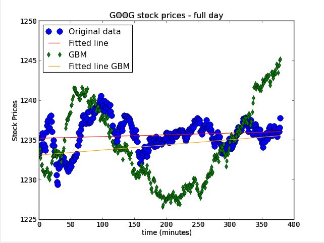
Figure 7.10: GOOG stock prices full Figure 7.11: Stock prices for minutes
day with GBM results 50 to 100 with GBM results.
t-statisitcs −0.1265631600773. t-statisitcs −0.034841261935855.
p-value 0.8993198087993637. p-value 0.9722771861891476.
Studying the figures that correlates to the GOOG share prices (original data), we can
see that the market trend changes throughout the day several times and consists of
much trading activity. As we can see in Figure 7.10, when the prices consists of many
trends, the GBM results starts “tight” around the real data, however, it doesn’t manage
to last for longer periods under market trend changes. As expected, the results of the
t-test for this single trend time fragment also demonstrate a significant improvement.
32
Technion - Computer Science Department - M.Sc. Thesis MSC-2020-16 - 20207.6 Observation fit as a function of sequence length
The third experiment we conduct to check how the data fits the model is to measure
the quality of the fit as a function of the sequence length. We score the fit level using
the p-value of a t-test.
Our test works as follows; First, we take a random subsequence of the data set of length
l time units. Then, we use Algorithm 1 to extract the market features (µ, σ) that fits the
subsequence. Then, we conduct the t-test on the GBM model for the given subsequence
of length l and (µ, σ). For each length l, we chose several different subsequences from
the data set for which the entire test is done and the result is the average p-value.
This is done in order to randomize the investigated subsequences for each length l and
thus to reduce noising affects such as stronger or weaker prices fluctuations in a specific
subsequence.
Figure 7.12: Model p-value as a function of sequence length
Figure 7.12 depicts the results of the described test. We perform this test three times
- with increasing amount of repetitions. The number of repetitions is the amount of
different subsequnces of prices being chosen for each length l, and for the amount of exe-
cutions of the GBM model for each such subsequence (r stands for repetitions). The test
was conducted using the GOOG security price during the dates of the 17,18,22/04/2019.
One can see that the ability of the GBM model to describe the data degradate with the
length of the sequence. This is due to the fact that the parameters (µ, σ) change over
time and thus the probability that a short sequence matches a specific GBM model is
higher.
33
Technion - Computer Science Department - M.Sc. Thesis MSC-2020-16 - 2020The Python function used in order to find the p-values is the “ttest ind” from the
“scipy.stats” library4 . The data used is the GOOG stock prices during the 17-22.04.2019,
the execution itself took 13 minutes and 58.18 seconds. The amount of repetitions is
as mentions on the graph itself (10, 50, 150).
4
The formal documentations from the SciPy project https://docs.scipy.org/doc/scipy/
reference/generated/scipy.stats.ttest_ind.html
34
Technion - Computer Science Department - M.Sc. Thesis MSC-2020-16 - 2020Chapter 8
Forecasting accuracy
8.1 Accuracy as a function of delay
A crucial part of this thesis goal is to asses the impact of HFT delay on their ability
to estimate securities prices correctly. In the previous sections, we investigated how to
use the GBM model and the feature extraction algorithm. In this section, We measure
the accuracy of our model as a function of the delay.
Assuming a security price is known at time t0 and we wish to act according to this price
(buy or sell). Our ability to “catch” this exact price is limited by our delay from the
stock exchange. Thus, our action will only take place on time td . The measurements
conducted in this section estimate the error size. We measure the effect of the standard
deviation of the GBM model in order to quantify its accuracy.
From Equation 4.12, and by the definition of standard deviation, we get that the
standard deviation of GBM is
√
Standard Deviation(GBM ) = σ ∗ ∆t. (8.1)
We perform an empirical test to check the actual behaviour of the model’s standard
deviation. We do so by executing the model multiple times. Each execution yields
a series x1 , ..., xn where xi is the value estimated for time t = i. Then, we find the
standard deviation for all the values xi in all the executions.
Since the examined standard deviation is merely an attribute of the model, the actual
values being assigned are of no significant and are only necessary in order to execute
the model. Thus, We perform the measurements using the (µ, σ) features found for the
time fragment in Figure 7.5 using Algorithm 1.
35
Technion - Computer Science Department - M.Sc. Thesis MSC-2020-16 - 2020Figure 8.1: Standard deviation as function of time units passed
As one can see in Figure 8.1, the standard deviation of the GBM model behaves as
√
expected and correlates with σ ∆t.
The importance of this result is that now we have a way to quantify the difference
between the price a trader see and the price this trader can realistically use as a function
of it’s time delay. From financial point of view, Equation 8.1 means that the price
difference grows linearly with the root of the trader’s time delay.
8.2 Accuracy of forecast
Since the prime goal of this thesis is to analyse potential HFT profitability with respect
to their latency, we measure the forecast mistake size as a function of the trader’s delay.
Namely, if one attempts to use the GBM model in order to estimate future security
prices, we want to quantify the size of the mistake in their estimates as a function of
their delay. Thus, in this section we focus on quantifying the mistake size as a function
of the delay.
This task might seem similar to the evaluation of the mistake as a function of the
sequence length in Section 8.1. However, this is not the case. The analysis in the
previous section was done using a fully known data set; That is, we considered the full
sequence to extract the market features. In contrast, the analysis in this section is done
using only the available data at the relevant time.
Our method to perform this check is as follows; First, we take a random sequence of
values of length l time units. Then, we divide it into two consecutive sequences. The
36
Technion - Computer Science Department - M.Sc. Thesis MSC-2020-16 - 2020first, is used to extract the market features using Algorithm 1. The second is compared
to the synthetic price series generated by applying the market features to the GBM
model GBM (x1 , µ, σ, n) 1 . The result is the average difference between xi = ln Si and
the log of the actual price at time t = i 2 . The first time sequence used for the feature
extraction is named the “train set” and the second consecutive sequence is called the
“test set”.
This study allows us to simulate a scenario in which a trader has access to a security
price data and is about to perform an action (buy/sell). Namely, the trader knows
the train set and the test set remains unknown. Since this trader is aware of having a
certain delay, he is required to estimate the future price of the security after a certain
time delay, when his order is executed in practice. The results of this study depicts the
average error between the log of the forecasted price the trader asses and the log of the
actual price.
Figure 8.2: Conducted on the AAPL Figure 8.3: Conducted on the GOOG
security prices during the 22.04.2019. security prices during the 17.04.2019.
Figure 8.4: Forecast Average accuracy as a function of time units amount
Figures 8.2 and 8.3 depicts the results of our study. We use a train set of 150 time
units, test set of 50 time units and 100 repetitions 3 . As one can see, the size of the
√
mistake behaves like σ ∆t. This is especially interesting since it the same behaviour
observed for the growth of standard deviation in Section 8.1, in spite the fact that the
data was not analysed while the market features were extracted (test set VS train set).
From these results, we conclude that for a short term, the accuracy of the GBM model
remains constant.
Next we want to study the effect of the sizes of the test sets on the results. Figure
1
x1 is the last price of the first sequence.
2
The average is done by both choosing several different data sequences and by executing the
GBM (x1 , µ, σ, n) several times for each data sequence.
3
100 different data sequences were used and for each of this data sequences 100 executions of the
GBM model were conducted.
37
Technion - Computer Science Department - M.Sc. Thesis MSC-2020-16 - 2020Figure 8.5: Forecast accuracy for longer test set. Conducted on GOOG prices during
the 17,18,22.04.2019
8.5 depicts the forecast accuracy behaviour for longer test set. As expected, one can
√
see that the σ ∗ ∆t behaviour breaks down as longer delays are exercised. In this
experiment, we also used 100 repetitions and train set of 150 time units. The 50 time
units vertical line indicts the point where the previous study ended. Also, one should
note that after the 150 time units vertical line, the average difference size starts to grow
faster.
We also check the effect of the train set length on how accurate the model forecast is.
In order to do so, we check the mistake size between the actual price and the forecasted
prices after three fixed time units amount - 5, 10, 20. Namely, we attempt to forecast the
price after each of this time units amount. This test results are depicted in Figure 8.6.
As one can notice, the significance of the the train set size is crucial at the beginning;
However, it decays quickly and then becomes irrelevant.
38
Technion - Computer Science Department - M.Sc. Thesis MSC-2020-16 - 2020Figure 8.6: Forecast mistake as a function of train set length. Conducted on GOOG
prices during the 17,18,22.04.2019
39
Technion - Computer Science Department - M.Sc. Thesis MSC-2020-16 - 202040 Technion - Computer Science Department - M.Sc. Thesis MSC-2020-16 - 2020
Chapter 9

                  Potential profitability due to low
                  latency

                  In this Section we use the AAPL security prices and the GOOG security prices as a
                  test case to examine the potential profit that can be made by HFT during a single day.
                  Note that our profit analysis is based on the time unit interval size of the data. In this
                  section two different methods to quantify potential profits are examined, both of which
                  relay on price changes size and frequency.

                  Our first goal is to answer the following basic question - “How likely is the GBM model
                  to correctly foresee a price change?”. Namely, if a HFT uses the sequence of prices
                  until the current price and then uses the GBM model to forecast whether the prices
                  is about to go up or down, how likely is the GBM model to be correct? In practice
                  though, a trader has a certain time delay before it can access prices information and/or
                  execution orders (we assume information access and execution order submission time
                  delay is equal). Thus, using a model to forecast whether a price is about to go up or
                  down immediately is of no use to the trader. Rather, the trader needs to know whether
                  the price is about to go up or down at a certain time in the future (specifically d time
                  units in the future, d being the size of the trader’s delay). Thus, if the traders submit
                  an execution order at time t = 0 it is actually executed at time t = d then we check
                  how accurate the GBM model is in forecasting a price change at this time range.

                  Figures 9.1 and 9.2 depicts the accuracy percentage as a function of the delay. The
                  results obtained by taking a data sequence and dividing it into a train set and a test set.
                  Then, after using Algorithm 1 to extract the market features, we executed the GBM
                  model, and then we checked for each time delay whether the model forecasts an incline
                  or decline compared to the last known price (the end of train set). Using the test set
                  we checked whether this forecast is correct or not. To remove noise, we choose multiple
                  data sequences and for each data sequence we executed the model several times, the

                                                               41

Technion - Computer Science Department - M.Sc. Thesis MSC-2020-16 - 2020
You can also read