Can Capital Deepening Explain the Global Decline in Labor's Share?
←
→
Page content transcription
If your browser does not render page correctly, please read the page content below

Staff Working Paper/Document de travail du personnel 2019-3

Can Capital Deepening Explain the
Global Decline in Labor’s Share?

by Andrew Glover and Jacob Short

Bank of Canada staff working papers provide a forum for staff to publish work-in-progress research independently from the Bank’s Governing
Council. This research may support or challenge prevailing policy orthodoxy. Therefore, the views expressed in this paper are solely those of the
authors and may differ from official Bank of Canada views. No responsibility for them should be attributed to the Bank.

                                                                                                               www.bank-banque-canada.ca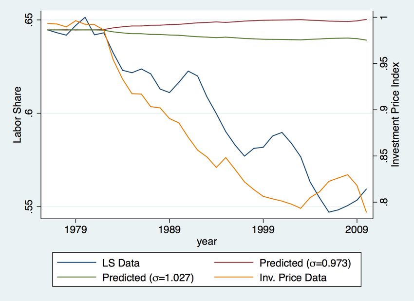
Bank of Canada Staff Working Paper 2019-3

                                  January 2019

Can Capital Deepening Explain the Global Decline
               in Labor’s Share?

                                        by

                    Andrew Glover1 and Jacob Short2

                             1 Departmentof Economics
                          University of Texas at Austin
                           Austin, Texas, USA 78722
                        andrew.glover@austin.utexas.edu

                         2Financial Stability Department
                                Bank of Canada
                       Ottawa, Ontario, Canada K1A 0G9
                           jshort@bankofcanada.ca

ISSN 1701-9397                                               © 2019 Bank of Canada
Acknowledgements
We are deeply grateful to Justin Barnette, Rui Castro, Oli Coibion, Jonathan Heathcote,
Igor Livshits, Lance Lochner, Jim Macgee, Salvador Navarro, Erwan Quintin, David
Rivers, and José-Víctor Ríos-Rull for helpful discussion and advice on earlier drafts of this
paper. We thank Loukas Karabarbounis and Brent Neiman for making their data on labor's
share and investment prices public. Any errors are our own.
iAbstract
We estimate an aggregate elasticity of substitution between capital and labor near or below
one, which implies that capital deepening cannot explain the global decline in labor's share.
Our methodology derives from transition paths in the neo-classical growth model. The
elasticity of substitution is identified from the cross-country correlation between trends in
the labor share and (a proxy for) the rental rate of capital. Trends in labor's share and the
rental rate are weakly correlated across countries, and inversely related in most samples.
Previous cross-country estimates of this elasticity were substantially greater than one,
which we show was partly due to omitted variable bias: earlier studies used investment
prices alone to proxy for the rental rate, whereas the growth model relates rental rates to
investment prices and consumption growth.
Bank topics: International topics; Firm dynamics; Labour markets
JEL codes: E25, E22, J3, E13
Résumé
Nous estimons une élasticité de substitution agrégée entre le capital et le travail qui est près
de ou inférieure à l’unité, ce qui signifie que l’intensification du capital ne peut pas
expliquer la baisse de la part du revenu attribuable au travail observée à l’échelle mondiale.
Notre méthode provient des sentiers de transition du modèle de croissance néoclassique.
L’élasticité de substitution est déterminée à partir de la corrélation entre les tendances de
la part du revenu attribuable au travail et du coût de location du capital (exprimé par une
variable d’approximation) pour divers pays. Ces tendances sont faiblement corrélées entre
les pays et négativement corrélées dans la plupart des échantillons. Les estimations
précédentes de cette élasticité étaient nettement supérieures à l’unité, résultat qui découle
en partie d’un biais dû à l’omission de variables : nous montrons en effet que les études
antérieures n’utilisaient que le prix de l’investissement comme variable d’approximation
du coût de location du capital. Or le modèle de croissance établit un lien entre le coût de
location, le prix des investissements et la croissance de la consommation.
Sujets : Questions internationales; Dynamique des entreprises; Marchés du travail
Codes JEL : E25, E22, J3, E13
iiNon-Technical Summary
The share of total income paid to workers (labor’s share) has been declining globally
over the past 30 years. Understanding this decline is important for two reasons: first,
prior to 1975, labor’s share was relatively constant, and many of the assumptions in
modern macroeconomic theories are tied to this constancy. Second, a fall in labor’s
share may have important implications for income and wealth inequality, which has
been rising over the same period of time.
A potential explanation of the decline in labor’s share is that, due to a fall in the price
of investment goods, countries accumulate greater amounts of capital inputs relative to
labor inputs. If capital and labor are substitutes in the production of final goods, then
this capital deepening can lead to a rise in the share of income paid as returns on
capital and a fall in labor’s share. The degree of substitutability between capital and
labor is pivotal. If capital and labor inputs are complementary inputs in production,
then greater accumulation of capital would lead to a rise in labor’s share. This potential
explanation has renewed macroeconomists’ interest in estimating the aggregate elasticity
of substitution between capital and labor.
Using the theory of capital demand of a profit-maximizing firm and cross-country
data, we estimate the elasticity of substitution from the correlation between country-
specific trends in rental rates of capital and labor’s share. We find that a unitary
aggregate elasticity of substitution between capital and labor is consistent with cross-
country data. This implies that capital and labor are not gross substitutes in production,
and that capital deepening cannot explain the decline in labor’s share. Furthermore, we
show that previous estimates using cross-country data are biased upwards (concluding
capital and labor are substitutes) because they omitted a theoretically and empirically
important variable related to consumption growth. Importantly, our finding reconciles
the previous cross-country evidence with the existing literature using firm-level data,
the bulk of which estimate that capital and labor are not substitutes.
21 Introduction
Historically, Kaldor’s stylized facts have supported a unitary elasticity of substitution
between capital and labor due to the near constancy of labor’s share of income (Kaldor
(1957)). As documented by Karabarbounis and Neiman (2014), this near constancy is no
more – labor’s share has declined globally since the 1980s. This downward trend, which
has occurred alongside rising income and wealth inequality (Piketty (2014), Piketty and
Zucman (2014)), has renewed macroeconomists’ interest in estimating the aggregate
elasticity of substitution between capital and labor (henceforth referenced as σ ≥ 0).
This parameter is pivotal: if it is smaller (greater) than 1 then anything that causes an
increase in the capital-labor ratio will increase (reduce) labor’s share. Specifically, if it
is significantly larger than 1, then the global decline in labor’s share can be explained
by capital deepening due to falling investment prices, as observed over the same time
period. Using a large cross section of countries, we estimate that σ ≤ 1 and conclude
that capital deepening cannot account for the global decline in labor’s share.
We identify σ from the capital demand function of a profit-maximizing firm in the
neo-classical growth model. This demand function implies that a 1% fall in the rental
rate of capital should reduce labor’s share of income by (σ − 1)%. The idea of the
cross-country estimation strategy is to correlate country-specific trends in rental rates
and labor’s share to estimate σ. Unfortunately, rental rates are not readily available
for a large cross section of countries, so we use the inter-temporal Euler equation for
investment to find a proxy. This condition implies that the rental rate depends on
the relative price of investment goods, as well as a transitional term that reflects the
gradual rise in consumption in response to lower investment prices. We estimate σ from
various data sources, cross-sectional samples of countries, and statistical models. Our
estimates are typically smaller than one (although statistically indistinguishable). The
average point estimate from our baseline specification is σ̂ = 0.973, which implies that
the global decline in investment prices should have increased labor’s share slightly.
Our results contrast sharply with two recent studies by Karabarbounis and Neiman
(2014) (henceforth KN) and the International Monetary Fund World Economic Outlook
(2017) (henceforth IMF). These studies also estimate σ from cross-country correlations
between trends in labor’s share and investment prices, but omit consumption growth
and assume that trends in the rental rate are identical to trends in investment prices.1
1
At least one earlier study estimates σ from cross-country data and finds a similar result to ours.
Backus, Henriksen and Storesletten (2008) use cross-country variation in corporate tax rates and capital-
output ratios to estimate σ ≈ 1. Their conclusion, which our estimates reaffirm, is that cross-country
3For example, KN estimate σ ≈ 1.26 and conclude that capital deepening due to falling
investment prices can account for half of the global decline in labor’s share. Similarly,
the IMF estimates that developed countries have an elasticity greater than one (although
they do estimate that emerging-market countries have an elasticity less than one). We
provide a full account of why our estimates differ from these studies in Section 6.
Our chief conceptual innovation relative to the KN/IMF studies is to proxy for rental
rates using their theoretical relationship with investment prices and consumption rather
than investment prices alone. While investment prices are a valid proxy for rental rates
in a steady state (i.e., after investment prices have been constant for a long time), the
data are clearly inconsistent with such an assumption: both consumption and invest-
ment prices exhibit trends that are significantly different from zero on average and vary
substantially across countries. Our proxy, which includes a transitional term reflecting
consumption growth, is valid along transition paths. We show, both theoretically and
empirically, that omitting the transitional term can substantially bias estimates of σ
away from one.2 Using our proxy for the rental rate reduces the absolute effect of in-
vestment prices on labor’s share of income, as mediated by rental rates, by more than
50% in cases and often reduces the effect to zero, both in terms of statistical significance
and economic magnitude.
Section 2.1 provides a theoretical basis for our rental rate proxy and the omitted
variable bias from excluding it, but a simple example provides intuition. Suppose that
σ is slightly above one3 and the relative price of investment follows a path of geometric
decline, eventually falling by 1% (i.e., the investment price falls by half of the remaining
distance each year). Households choose a smooth path of consumption to the new
steady state, along which consumption growth is declining, which causes rental rates to
transition slower than investment prices. The path of consumption implies a slow rise in
the investment rate and gradual capital deepening. An econometrician whose data start
late in the transition will observe an essentially flat path for the investment price but a
downward trend in labor’s share. If the econometrician ignores the trend in consumption
growth, they will underestimate the decline in rental rates and erroneously infer a large
value of σ.4
The above intuition aligns with our empirical results. Estimates of σ from our base-
variation in corporate tax rates cannot account for the variation in capital accumulation across countries.
2
The bias is upward (downward) if the true value of σ is greater (smaller) than one.
3
This logic works symmetrically and introduces downward bias if σ is below one.
4
There will be some degree of omitted variable bias unless the data happen to contain the entirety
of every country’s transition path.
4line sample of countries are below one and shrink when we omit the transitional term. In
samples for which σ̂ > 1, omitting the transitional term leads to larger point estimates,
and the opposite holds for samples in which σ̂ < 1. This is true across specifications,
estimators, and samples. In short, cross-country data exhibit a weak correlation between
labor’s share and rental rates (once consistently proxied), which implies that σ is near
one.
Our proxy overcomes the omitted variable bias discussed above, but may introduce
additional measurement error since it requires new data on consumption, and requires
us to specify a utility function. We address this concern in two ways. First, we use
investment prices as an instrument for our rental rate proxy. As long as the addi-
tional measurement error in our proxy is independent from the measurement error in
investment prices, this cleanses our estimates of any extra attenuation bias relative to
using investment prices alone. Second, we estimate the elasticity of substitution from
subsamples with higher-quality time series data, such as developed or Organisation for
Economic Co-operation and Development (OECD) countries and those with longer time
series. We expect such countries to have less measurement error in investment prices in
the first place, as well as better consumption data. Reassuringly, we estimate elasticities
for these countries that do not differ significantly from our pooled estimates.5
The cross-country approach we employ is one of three empirical strategies used to
identify the aggregate elasticity of substitution. One alternative, pursued by Antràs
(2004), uses aggregate time series variation in the United States and estimates σ ≤ 1,
but requires imputation of effective capital to labor ratios in the presence of factor-
augmenting technological growth. There is also a large literature on estimating the
elasticity of substitution from micro data. A particularly relevant example is Oberfield
and Raval (2014), who estimate these micro elasticities and aggregate them to compute
a σ substantially below one in the United States.6 This approach is the most precise,
but also requires high-quality micro data that are unavailable in many countries. The
benefit of the cross-country approach is that it requires only aggregate data on quantity
flows and relative prices, but has thus far yielded substantially higher estimates of σ than
the other two strategies. Our estimates effectively reconcile the cross-country approach
with the other two, while retaining its broad applicability.
5
We also emphasize that most of our point estimates are slightly below one. If we could fully eliminate
all measurement error, then we would expect most estimates to fall further below one and therefore
strengthen our substantive conclusion.
6
Chirinko (2008) and León-Ledesma, McAdam and Willman (2010) provide surveys of the literature
on estimating the elasticity of substitution. The majority of estimates are below one.
5Although our estimates of σ indicate that capital deepening has not caused the global
decline in labor’s share, the fact that it has fallen so broadly warrants an explanation.7
Our estimates lend support for explanations that do not require strong capital-labor
substitutability to generate a decline in labor’s share. Some examples include Autor
et al. (2017) and Kehrig and Vincent (2017), who document that labor’s share has fallen
along with a rise in product-market concentration; Elsby, Hobijn and Şahin (2013), who
estimate a strong correlation between industry-level trends in labor share and import
competition; Grossman et al. (2017), who build an endogenous growth model with hu-
man capital in which labor’s share falls due to slower productivity growth; and Glover
and Short (2015), who estimate that an aging workforce reduces labor’s share at the
industry level.
We proceed by outlining the structural theory that relates labor’s share to investment
prices and show the economic importance of σ ≈ 1 in that framework. We derive the
appropriate reduced form model to estimate σ, then present our estimates, perform
robustness tests, discuss previous estimates, and conclude.
2 Labor’s Share in Theory
Our framework to estimate σ is based on transition paths in the neo-classical growth
model. The relative price of investment goods in country i follows an exogenous and
deterministic path to a new steady state, P i . Starting at an initial P0i , which may or
may not be a steady state, the path is written as:
log Pti = log P i + log ξti , (1)
where P i is the eventual steady state investment price and log ξti is a sequence that tends
to zero (i.e., log ξti describes the transition path of investment prices). We think of the
data as representing, for each country, a snapshot of such a transition path.
We assume that goods and factor markets are competitive.8 Each country is popu-
7
While some of the decline may be due to mis-measurement or statistical imputation (see Rognlie
(2015) for a discussion of housing’s effect on capital’s share; Bridgman (2014) on the importance of
measuring depreciation and production taxes; Elsby, Hobijn and Şahin (2013) for a discussion of al-
locating proprietor’s income between factors; and Koh, Santaeulàlia-Llopis and Zheng (2016) on how
changing treatment of income from intellectual property affected labor’s share in the U.S.), we expect
these measurement issues to be alleviated by studying labor’s share of the corporate sector wherever
possible and using a broad cross section of countries at different points in development.
8
Allowing for goods market markups is straightforward in theory, but introduces capital’s share
6lated by a large number of representative households, each of which chooses sequences
of consumption ct , labor nt , bonds bt , and investment xt to solve the problem:
∞
X
max β t u(ct , 1 − nt ) (2)
(ct ,nt ,xt ,kt+1 ,bt+1 )∞
t=0
t=0
subject to:
ct + Pti xt + Qit bt+1 = Rti kt + Wti nt + bt (3)
kt+1 = (1 − δ)kt + xt (4)
k0 , b0 given. (5)
We denote the price of a risk-free bond as Qit , the real wage by Wti , and the rental
rate for capital by Rt . We are intentionally agnostic about the determination of Qit and
Pti . For Qit , our estimation approach remains valid whether the bond market is closed
and Qit is determined in equilibrium or each country is a small open economy and takes
Qit exogenously. Likewise, it does not matter if the price of investment goods changes
because each country experiences idiosyncratic shocks to the production technology for
investment goods or if they face exogenous changes in the price of investment goods on
the international market.
We will make use of the inter-temporal Euler equations
i i
1 Rt+1 + (1 − δ)Pt+1
= , (6)
Qit Pti
1 uc cit , 1 − nit
= . (7)
Qit βuc cit+1 , 1 − nit+1
The first is a no-arbitrage condition between the gross rates of return on bonds and
investment and the second relates growth in marginal utility to the return on bonds.
Combining these two equations yields a relationship between the rental rate, investment
prices, and growth in the marginal utility of consumption:
uc cit , 1 − nit Pti
i i
Rt+1 = Pt+1 i +δ−1 . (8)
βuc cit+1 , 1 − nit+1 Pt+1
A representative firm rents capital and hires labor to produce consumption goods
and profit’s share of income as distinct variables. These cannot be separated in the data, so require
imputation. In Appendix 1, we estimate σ using an imputation procedure suggested by KN. The
estimates are similar to our baseline under perfect competition, but are subject to (potentially large)
measurement error.
7using a constant returns to scale production function, which we assume has a constant
elasticity of substitution
σ
σ−1
σ−1 σ−1
Yti = αki Ait Kti σ
+ (1 − αki ) Bti Nti σ
, (9)
where σ is the elasticity of substitution between capital and labor and is the parameter
of interest in this paper, as it determines the effect of investment prices on factor shares.
The firm’s capital demand equation is the basis for our empirical model and is given by:
σ1
Yti
σ
Rti = αki (Ait ) σ−1 . (10)
Kti
Denoting labor’s share of income as sit ≡ 1 − RYt K
t
t
, the theoretical relationship between
rental rates and labor’s share can now be written as:
σ−1
Ait
1− sit = (αki )σ . (11)
Rti
All else being equal, a rise in the rental rate of capital will cause labor’s share to rise
(fall) when σ is greater (smaller) than one. If we had data on the rental rate, Rti , then
we could use Equation 11 to estimate σ. These data are not readily available, however,
so we use Equation 8 to proxy for the rental rate. Combining Equations 8 and 11, we
relate labor’s share to investment prices and consumption:
∆ log(1 − sit ) i i i
= (σ − 1) ∆ log At − ∆ log Pt − ∆ log ζt , (12)
where ζti is the transitional term:
i i i
uc (Ct−1 , 1 − Nt−1 ) Pt−1
ζti = + δ − 1. (13)
βuc (Cti , 1 − Nti ) Pti
Finally, we express the left-hand side in terms of labor’s share rather than capital’s
share:9
si
∆ log(1 − sit ) ≈ − ∆ log sit , (14)
1 − si
where xi is the average of variable x for country i over the years for which it is observed.
9
This approximation is expositional, so that we reference correlations with labor’s share rather than
capital’s share. We estimate similar σ̂ without the approximation.
8This gives Equation 15, which will be the theoretical basis for our baseline estimating
equation in Section 5.
si i i i i
∆ log st = (1 − σ) ∆ log At − ∆ log Pt − ∆ log ζt . (15)
1 − si
2.1 Bias From Omitting the Transitional Term
We now explain how omitting the transitional term biases estimates away from one in
the growth model. This is because both the transitional term and labor’s share change
more gradually than investment prices. The transitional term falls as investment prices
decline, but does so slowly because households smooth consumption. Labor’s share
changes more slowly than investment prices because it requires the capital-labor ratio
to rise, which takes time because capital is a stock variable. In Section 5, we show that
this is relevant for our empirical estimate of σ.
We think of country i’s path beginning from arbitrary values of K0 and P0 as the
economy converges to a new steady state in response to a fall in the price of investment
goods. We assume inelastic labor supply and close the model from Section 2 with an
aggregate feasibility constraint and time series for investment prices, which requires that
we add the following equations:10
Cti + Pti Xti = Yti , (16)
log Pti = log Pt−1
i
+ log ξti , (17)
log ξti = ρ log ξt−1
i
+ (1 − ρ)∆ξ . (18)
Equation 18 specifies the transition path of investment prices, which slowly change by
100∆ξ percent.
We assume preferences are separable between consumption and leisure and that the
intertemporal elasticity of consumption is one. All other parameter values are listed
in Table 1. The most important is σ, which we assume to be slightly above one at
σ = 1.01. We then check whether estimates σ̂ from two specifications of Equation 15
(with ζ included and omitted) can accurately recover σ. We do this by varying our first
data point, t0 ∈ {3, ...10}, and then estimating σ using 20 years of the transition path.11
10
This is equivalent to a two-sector model with a linear technology that transforms consumption
goods into investment goods.
11
We consider σ = 1.01 because previous cross-country estimates have omitted βζi and found elastic-
ities greater than one. The bias would be downward if we set σ < 1.
9We begin by plotting time series of the log investment price, log capital’s share, and
log ζ in order to provide intuition for how investment prices and ζ are predicted to covary
along the transition path. These series are found in Figure 1. The investment price falls
substantially early on and is then quite flat, while capital’s share rises more gradually.
Clearly, if an econometrician correlates trends in capital’s share and investment prices
and their time series begin after the first few years, then they compare an extremely
slow decline in investment prices (nearly flat) to a positive trend in capital’s share. They
would therefore infer a large value of σ rather than the value of 1.01 used to generate
the series. If they include the trend in ζ, however, then they will realize why capital’s
share continues to rise after investment prices flatten out – it is mirrored by a gradual
fall in ζ.
We quantify this intuition by calculating the elasticities directly under the fully
specified model (assuming we know the utility function and parameter values) and then
under the misspecified model with ζ omitted. We calculate σ using the same procedure
from the model: we first estimate the growth rates of each variable from log xt = β0 +
βx t + ηxt and then use these growth rates, βx , to calculate σ. We define the elasticities
calculated from the exact and omitted models as:
σ̂e = 1 − β1−s βP + βζ , (19)
β1−s
σ̂o = 1 − . (20)
βP
The bias is plotted in Figure 2, measured as 100 σ̂iσ−σ . As expected, σ̂e is near
σ = 1.01 no matter when the data begin (the flat line in Figure 2), while the misspecified
estimate exhibits substantial upward bias.
3 Economic Importance of σ ≈ 1
Our estimates of σ are often statistically indistinguishable from one and our baseline
estimates are below one on average, but it is useful to quantify the economic importance
of σ slightly above one, which is consistent with the upper bound of our confidence
intervals. Figure 3 plots the series for global labor’s share and investment prices against
predicted labor’s share for σ = 0.973 and σ = 1.027. These predicted series correspond
to the average of our baseline point estimates and the average of the upper bound of the
95% confidence intervals for those estimates. Table 2 contains the cumulative change in
10predicted global labor’s share for each of these elasticities. In each case, the predicted
change in labor’s share is small due to the elasticities being near one.
Whether a large share of the global decline in labor’s share can be explained by
capital deepening due to declining investment prices therefore rests on whether σ is
substantially greater than one. We now estimate σ using various series, samples, and
empirical models. The overwhelming majority of estimates indicate that σ is near one
and, if anything, smaller.
4 Data
Our data set is an unbalanced panel containing 104 countries with data available for
some years between 1975 and 2010, which was used by KN. The panel includes data on
labor’s share, investment prices, and aggregate consumption. We will focus on medium-
to long-run trends, rather than estimate σ from year-to-year variation.12 We first obtain
measures, for each country, of the medium- to long-run trends in the time series of each
variable (we refer to this as the “first step”). We then estimate σ in Equation 15 from
the cross section of trends constructed in the first step (we refer to this as the “second
step”).
4.1 Description of Variables
We first describe the series for the first step and then describe the measure of the long-
run trends used in the second step. For the first step, we need time series for the relative
price of investment goods, labor’s share, and consumption for each country.
For the relative price of investment goods, we present results from two publicly
available series: the Penn World Table (PWT) and the World Bank’s World Develop-
ment Indicators (WDI). For labor’s share of income we consider a hybrid measure that
uses corporate-sector labor’s share whenever available and an economy-wide measure
of labor’s share when corporate data are missing.13 The measure of labor’s share uses
corporate labor’s share when available because it is cleaner: it avoids the difficulty of
12
Our data construction and focus on medium- to long-run trends are shared by KN and the IMF.
For all samples and specifications, point estimates using year-to-year changes are consistently near one
and never statistically different.
13
The labor’s share series include time series constructed from country-specific sources, as well as
series from OECD and UN data sets. We will present estimates using each labor’s share series, as well
as the unadjusted OECD/UN measures.
11allocating proprietor’s income between labor and capital. The hybrid series is our base-
line in order to maximize sample size in the second step, although we get similar results
using only corporate labor’s share, as seen in Table 9.
To construct the transitional term, we use real per-capita consumption from the
PWT. We then assume a utility function that is separable between consumption and
c1−θ
leisure, with a constant inter-temporal elasticity of substitution: u(ct , 1 − Nt ) = 1−θ t
+
ν(1 − Nt ). Our baseline further restricts these preferences to be consistent with balanced
growth, so that θ = 1 and uc (ct , 1 − Nt ) = c−1 t . Finally, we set δ = 0.10 and β = 0.91,
although we have verified that our estimates are robust to these values.14
For country-year observations where consumption growth is sufficiently small, ζti mea-
sured by Equation 13 may be negative and log ζti undefined. Country-year observations
for which log ζti is undefined are dropped (this typically amounts to fewer than 2% of
country-year observations, as reported in Table 3). Since we must drop a small share of
country-years for which ζti is undefined, we also report estimates using the ex-post real
interest rate as a proxy for βUcU(cc (c t ,`t )
t+1 ,`t+1 )
. Data on the real interest rate come from the
World Bank’s WDI, and is measured as the deposit rate less the growth rate of the gross
domestic product (GDP) deflator.15 The real interest rate has the advantage of being
independent of preference parameters, θ and β, but interest rates are not available for
all countries in our sample.
In the first step of estimation, we extract the long-run trend for each time series xit
described above, for each country i, by estimating βxi via ordinary least squares (OLS):
log xit = aix + βxi t + ηx,t
i
. (21)
We then have a triplet of these coefficients, (βsi , βPi , βζi ), for each country, which represent
annual growth trends in each variable.16
In Table 4, we present summary statistics for trends in investment prices, the tran-
sitional term ζ, the resulting rental rate proxy, and the predicted rental rates from the
first stage of our instrumental variable (IV) regression. On average, the trends in each
price series and transitional term are negative, but there is substantial heterogeneity.
We emphasize two patterns. First, the rental rate is substantially more volatile than in-
14
We have also estimated the model with different values of θ and obtained similar results. Especially
interesting is the case when θ = 0, so that βζi = 0 for all countries, and investment price trends alone
proxy for rental rates. Even this specification yields an estimate of σ near one for many samples (see
Table 13, columns “Tmin = 10” and “Tmin = 20”).
15
Estimates are robust to using lending rates and consumer price index (CPI) growth.
16
We refer to these estimates as βxi rather than β̂xi to save notation.
12vestment prices alone, even after we cleanse it of extra measurement error by projecting
it onto investment prices. Second, the correlation of prices (and therefore our cleansed
rental rate proxy) is near zero for both series, though slightly negative for this sample.
Taken together, these two moments explain why we find an elasticity of substitution
(slightly) below one and why omitted variable bias generates estimates further from one
when investment prices alone proxy for rental rates.
4.2 Sample Selection
Sample selection poses a tradeoff between time series length in the first step and cross-
sectional sample size in the second step. The threshold for a country’s inclusion in the
second step is the length of its investment price and labor’s share time series, Tmin . On
the one hand, we want enough years of data to calculate long-run trends. On the other
hand, we want as many countries in the second step as possible, so we do not want to
set Tmin too high.17 Our preferred threshold drops countries with fewer than 10 years
of labor share and investment price data, which leaves us with 77 − 86 countries for
estimating Equation 15, depending on which labor’s share and investment price series
we use.
5 Estimation Results
In order to derive an empirical regression model, we assume that Ait consists of a world-
wide trend, γ, and a country-specific trend, εi :
1
log Ait = i
γt + ε t . (22)
1−σ
The reduced-form regression equation corresponding to Equation 15 is given by:
si
βs = γ + (σ − 1) βP + βζ + εi .
i i i
(23)
1−s i
We assume that country-specific trends in capital-augmenting productivity (εi ) are
uncorrelated with average investment price growth and estimate Equation 23 by in-
strumenting the sum βPi + βζi with βPi . This approach ensures that we identify σ from
17
Setting Tmin low also introduces more emerging-markets countries for which data may be poor and
therefore attenuate estimates of σ. We address this concern by estimating σ separately for developed
and emerging-market economies and by considering a broad range of Tmin for robustness.
13cross-sectional variation in rental rates induced by variation in investment price trends,
while also correcting for measurement error introduced by βζi . Our baseline regressions
have strong instruments, with a minimal first-stage F statistic of 41.1.
Table 5 reports our estimates for each combination of labor’s share and investment
price series. The point estimates of σ are typically below one and the average across
data sets is σ̂ = 0.973. All point estimates are near and statistically indistinguishable
from one; capital deepening due to declining investment prices cannot account for the
global decline in labor’s share.
5.1 Bias From Omitting βζi
We have discussed the importance of transitional dynamics (i.e., βζi ) for consistently
estimating σ in Section 2.1, which can be understood empirically as a form of omitted
variable bias. The relationship between the point estimate when βζi is omitted, σ̂ OM ,
and the true elasticity, σ, is given by18
V (βPi ) + CV (βPi , βζi )
σ̂ OM − 1 = σ − 1 . (24)
V (βPi )
This equation shows that the overall effect of a declining rental rate on labor’s share,
σ − 1, is biased away from the true effect by a scaling factor greater than one as long
as investment prices and the transitional term are positively correlated. In our baseline
sample using the PWT investment price series, the cross-sectional variance of βPi is 5.7%
and the covariance between βPi and βζi is 4.6%, which generates a scaling factor of 1.8
(i.e., σ̂ OM − 1 is biased away from σ − 1 by 81%).
Table 6 shows that omitting βζi generates smaller σ̂ for each data set, except for the
KN-WDI data when σ̂ = σ̂ OM = 1.000. For each series, βζi and βPi are positively
correlated. Therefore, if σ is slightly below one in reality, as suggested by our IV
estimates, then omitting βζi introduces downward bias in σ̂. On the other hand, if
σ > 1, as estimated in previous studies, then omitting βζi introduces upward bias.
5.2 Measurement Error
We are concerned with measurement error, which would bias our estimates of σ towards
one. The main issue is that our rental rate proxy includes the transitional term ζ, which
18
The formula in Equation 24 is exact for the OLS estimator, but qualitatively useful for our IV
estimates, which we prefer because of measurement error in βζi .
14is measured with error above and beyond investment prices themselves. This motivated
our use of investment price trends as instruments for our rental rate proxy in order to
cleanse our proxy from any additional measurement error introduced by ζ. To see this
point, let ψPi be the measurement error in βPi and ψζi be the measurement error in βζi .
Then the IV estimate, σ̂ IV , is given by
cov(βPi + βζi , βPi )
σ̂ IV − 1 = (σ − 1) . (25)
cov(βPi + βζi , βPi ) + var(ψPi ) + cov(ψPi , ψζi )
We have no reason to expect the measurement errors in βPi and βζi to be correlated, so
the IV estimator is attenuated towards zero only through variation in investment prices.
That is, including ζ in our proxy for rental rates and instrumenting with investment
price trends introduces no additional attenuation relative to investment prices alone,
while overcoming the omitted variable bias from excluding it.
While we cannot quantify how much measurement error is left in investment price
trends, we now show that our point estimates are similar across subsamples with lower-
and higher-quality data. From this we conclude that measurement error in investment
price trends is either small, or that it is constant across countries that differ dramatically
from one another. We first estimate σ for developed/OECD countries separately from
emerging markets/non-OECD countries. Table 7 presents estimates of σ for developed
and developing countries separately. Developed countries have a slightly higher point
estimate on average, but neither elasticity is significantly different from one. Table 8
shows the same pattern for OECD and non-OECD countries. We therefore find no
evidence that σ varies significantly by development status or data quality.
This slice of the data is interesting beyond our check for measurement error, because
the elasticity of substitution may depend directly on a country’s development level. For
example, the elasticity may change as a country becomes more developed and adopts
new technologies. Whether the elasticity rises or falls with development is an open
question and there is conflicting evidence regarding the effect of development on σ.
Oberfield and Raval (2014) estimate a higher elasticity for India than for the United
States, while the IMF estimates a higher elasticity for developed than for emerging-
markets countries.19 Our estimates indicate that developed countries have an elasticity
indistinguishable from one and that developing countries may have a somewhat lower
19
Oberfield and Raval estimate establishment-level elasticities and then aggregate using input-output
tables, so differ substantially from us methodologically. The IMF uses an approach closer to ours, but
omits βζi , which we discuss in Section 6.2.
15elasticity, though the differences are small and statistically insignificant.
In summary, we have used an IV estimator to alleviate concerns of additional mea-
surement error from βζi . Investment price trends may still cause attenuation, but what-
ever is there must not vary substantially across countries with differing data quality. We
therefore think our point estimates of an elasticity slightly below one are compelling,
although emphasize that further eliminating measurement error would push most of our
estimates further below one. This strengthens our conclusion that declining investment
prices have not driven the global decline in labor’s share.
5.3 Capital-Augmenting Technology and Investment Prices
A remaining source of bias in σ̂ is the possibility of correlation between capital-augmenting
technological growth and investment prices (i.e., εi and βPi ). If capital-augmenting tech-
nology growth is negatively correlated with investment price trends, then our point
estimates will be biased away from one. Since we have estimated σ ≈ 1, the resulting
bias would be small and only further dampen the effect of investment prices on labor’s
share in either direction. However, if ν i and βPi are positively correlated, then our point
estimates are biased towards one. Since most of our estimates put σ slightly below one,
correcting for this bias (if it is there) would further align the cross-country with previous
identification strategies that typically estimate σ < 1, without changing our substantive
conclusion that investment price trends cannot account for the global trend in labor’s
share of income.
5.4 Further Robustness
We now explore the robustness of our estimates to alternative measures of labor’s share,
definitions of ζ i , subsamples of countries, and regression methods. The overwhelming
majority of estimates indicate an elasticity near or below one.
We first estimate σ using corporate labor’s share rather than the economy-wide
labor’s share measure from our baseline, the results of which are reported in Table 9.
This alleviates concerns about changes in proprietor’s income, which has been shown
to have large effects on the trend in labor’s share in the U.S. (Elsby, Hobijn and Şahin
(2013)). On the other hand, this reduces our sample size because some countries (mostly
emerging markets) do not have data for corporate labor’s share. Our point estimates
rise slightly on average, to σ̂ = 1.009, but the implied effect of investment prices on
labor’s share is still economically and statistically insignificant.
16We next consider an alternative measure of ζti , since this term required us to assign a
utility function and extra parameter values. We instead proxy for the ratio of marginal
utilities using a measure of the real risk-free interest rate by setting
i
Pt−1
ζti = (1 + rti ) + δ − 1, (26)
Pti
where 1 + rti ≡ Qi1 . This definition is agnostic about the utility function of the house-
t−1
hold, as well as the discount factor, but still requires a value of δ, which we set at 0.10 as
in the baseline. As reported in Table 10, our point estimates fall under this specification,
especially when using the WDI investment price series, and the average is σ̂ = 0.948.
Estimates of σ using real interest rates imply that the global decline in investment prices
should have increased labor’s share even more than implied by our baseline estimates.
We next estimate σ from alternative cross-sectional samples by varying our exclu-
sion restriction Tmin ∈ {5, 6, ...20}. It is useful to consider the effect of Tmin for both
economic and statistical reasons. Economically, there may be substantial cross-country
heterogeneity in capital-labor substitutability, which would require us to make any state-
ment about the effect of investment prices on labor’s share contingent. Statistically, we
further explore the tradeoff between sample size and data quality, since lower values of
Tmin increase our cross-sectional sample size, but higher values give longer time series to
i
calculate βLS , βζi , and βPi . Figure 4 plots each point estimate and 90% confidence interval
across all of our data sets. Estimates of σ using the PWT’s price series vary only slightly
as we change samples, consistent with a near-constant elasticity of substitution across
countries, while the WDI-based estimates rise and then fall across samples. Overall, only
6.25% (4 of 64) of point estimates are significantly above one in the statistical sense and
most (43 of 64) are below one in value.
Finally, we consider the effect of outliers on σ̂ by using the robust regression estimator
of Li (2011). Intuitively, this method fits OLS to the data, then weights each observation
as a function of its distance from the OLS line and a user-supplied tuning parameter,
and then estimates a weighted OLS regression. This procedure is iterated upon until
convergence. Robust regression is useful if one believes that the regression errors are
non-normal, but is otherwise less efficient than OLS; the tuning parameter allows the
user to balance this tradeoff. Table 11 compares our baseline estimates of σ to those
from robust regression, using a bold tuning parameter and a conservative one.20 The
20
A lower value of the tuning parameter down-weights outliers more severely and is more likely to
drop observations at early iterations of the algorithm by setting their weight to zero. Our bold tuning
17average point estimate is essentially identical across procedures and all estimates are
statistically insignificant from one.
In summary, cross-country trends in investment prices and labor’s share suggest that
the elasticity of substitution between capital and labor is less than or equal to one. The
global decline in labor’s share cannot be accounted for by capital deepening in response
to falling investment goods prices.
6 Comparison With Previous Estimates
Previous cross-country estimates that identify σ from investment price and labor share
trends argue that declining investment prices can account for much of the decline in
labor’s share, either globally or for a subset of countries. We now reconsider these find-
ings using our methodology. Accounting for transitional dynamics brings these previous
estimates much closer to our own. On balance, there is little cross-country evidence for
σ substantially above one.
6.1 Karabarbounis and Neiman, 2014
KN use the same data set and theoretical framework as us, but estimate a much larger
value of σ ≈ 1.26 and conclude that investment prices can account for half of the global
decline in labor’s share since the early 1980s. Our estimation procedure differs from
theirs in three ways. First, our proxy for rental rates includes the transitional term, βζi .
Second, they report estimates from a robust regression estimator, whereas our baseline
uses linear instrumental variables. Finally, we estimate σ from a larger cross-sectional
data set than KN because we include all countries with time series longer than Tmin = 10,
whereas they require Tmin = 15. We consider the importance of each of these choices.
We first present summary statistics for the KN sample. Table 12 shows that invest-
ment price trends are somewhat less variable for this smaller cross-sectional sample, but
still understate the cross-sectional variation in rental rate trends, even after correcting
for measurement error. Furthermore, the correlation between investment prices and la-
bor’s share is positive in this sample, but still very low. In fact, our preferred rental
rate proxy is actually more positively correlated with labor’s share than are investment
prices alone.
value is the default value implemented by Stata, which is near the lower bound suggested by Goodall
(1983), and the only estimator reported by KN. Our conservative value is the upper bound suggested
by Goodall (1983).
18Using a theoretically consistent proxy for rental rates is our most economically im-
portant difference with KN and has large effects on σ̂, which we isolate by estimating
the model with βζi included, but using the same cross section of countries and the same
robust regression estimator as KN. Specifically, we first estimate KN’s exact specifica-
tion, which we are able to match precisely in the column “KN” in Table 13, the average
of which is σ̂ = 1.26. We then save the weights produced by the robust regression algo-
rithm and use them to estimate a weighted regression with our interest rate proxy on the
right-hand side, the results of which are listed in column “Include βζi ”.21 The average
estimate falls from σ̂ = 1.26 to 1.11, which means that the effect of investment prices
on labor’s share is reduced by nearly 60%. While the omitted variable bias calculation
is invalid for the robust regression estimator, the reduction in σ OM − 1 is in line with
the scaling factor we calculated in Section 5.1.
The choices of estimator and sample selection are also important. The “IV” column
of Table 13 reports σ̂ from samples with Tmin = 15 but using the IV estimator from
our baseline rather than the robust regression estimator. This reduces the average point
estimate further to σ̂ = 1.07 and, for the PWT data, reduces the elasticity to one. As
we discussed in Section 5.4, the robust regression estimator with Stata’s default tuning
parameter severely down-weights outliers. In the case of the PWT investment price
series, for example, it puts zero weight on three countries, effectively reducing the cross-
sectional sample size. KN’s original rationale for relying exclusively on this specific
robust regression estimator was that their cross-sectional sample size was small. We
therefore find it useful to directly assess the effect of sample size by varying Tmin .
Our baseline results used a larger cross-sectional sample by setting Tmin = 10, so
within that larger sample we’ve already shown that σ ≈ 1 if estimated with a transition-
consistent proxy for the rental rate and a standard linear regression framework. We
therefore use the robust regression estimator and omit βζi when estimating σ on this
larger sample, which is shown in column Tmin = 10 of Table 13. The point estimates of
σ are near one, with some above and some below. Economically, these point estimates
imply little to no effect of investment prices on labor’s share. Statistically, they are indis-
tinguishable from one with relatively tight standard errors (smaller than the Tmin = 15
sample used by KN). Finally, since the added countries may have more measurement
21
The robust regression estimator would re-weight countries in the specification with βζi included.
We have kept the weighting matrix constant across these specifications in order to test these difference
between σ̂ OM and σ̂. We compute Z-statistics of −1.71, −2.16, −1.43, and −2.37 as we move down the
rows in Table 13. Our rental rate proxy therefore reduces the economic effect of investment prices on
labor’s share, typically with strong statistical significance.
19error when setting Tmin = 10 instead of 15, we report the same robust regression esti-
mates of the misspecified model with a smaller (but higher-quality) sample in column
Tmin = 20 and again find estimates close to one (although with larger standard errors
due to the smaller sample).
In summary, KN estimated a large value σ ≈ 1.26 and concluded that capital deepen-
ing due to falling investment prices could therefore account for half of the global decline
in labor’s share. This large estimate is at odds with other identification schemes, as well
as the cross-country estimates of Backus, Henriksen and Storesletten (2008). This dis-
crepancy is due to model specification, the weighted estimator, and an atypical sample.
Changing any one of them brings the cross-country estimates of σ closer to previous
studies (and to our baseline estimates).
6.2 IMF WEO, 2017
The IMF’s World Economic Outlook (2017) find conditional evidence that declining
investment prices reduce labor’s share. Using data from 1992 to 2014, the IMF estimates
that labor’s share falls in response to declining investment prices in developed countries,
although the opposite is true for emerging markets and these two responses offset one
another when developed and emerging market countries are pooled.
The role of investment prices in reducing labor’s share is further limited when we
account for the transitional term. In Table 14 we estimate the IMF’s partial-elasticity
model for each group of countries, but with βζi included in the proxy for rental rates.22
The column labeled “IMF” in Table 14 shows that the IMF estimates a larger difference
between developed and emerging-market countries than we found in Section 5.2, while
column “IV” of Table 14 shows that the estimates move closer to and are insignificant
from zero if we account for the transitional term, βζi , as in our baseline (using βPi as
an instrument). Most importantly, we estimate a much lower and insignificant partial
elasticity for developed countries, indicating that even their decline in labor’s share
cannot be accounted for by capital accumulation due to falling investment prices.
22
The IMF’s regression model does not identify σ because they use percentage-point changes in labor’s
share rather than percentage changes, which is why we call their estimates “partial elasticities.”
207 Conclusion
The aggregate elasticity of substitution between capital and labor is central to under-
standing the effect of capital accumulation on factor shares of income. The global decline
in labor’s share has drawn substantial attention to this parameter – if it is sufficiently
above one, then the observed decline in investment prices provides a simple explanation
for the decline in labor’s share. We have shown how to consistently estimate this elastic-
ity by using a theoretically derived proxy for rental rates, which depends on investment
prices as well as consumption growth. Our estimates indicate that σ is near one and, if
anything, below. We conclude that the global decline in labor’s share has occurred for
reasons other than capital deepening in response to declining investment prices.
21References
Antràs, Pol. 2004. “Is the US Aggregate Production Function Cobb-Douglas? New Es-
timates of the Elasticity of Substitution.” Contributions to Macroeconomics, 4(1): 1–
34.
Autor, David, David Dorn, Lawrence F Katz, Christina Patterson, John
Van Reenen, et al. 2017. “Concentrating on the Fall of the Labor Share.” IZA
Institute of Labor Economics Discussion Paper, 10539.
Backus, David, Espen Henriksen, and Kjetil Storesletten. 2008. “Taxes and the
Global Allocation of Capital.” Journal of Monetary Economics, 55(1): 48–61.
Bridgman, Benjamin. 2014. “Is Labor’s Loss Capital’s Gain? Gross Versus Net Labor
Shares.” Bureau of Economic Analysis BEA Working Paper 0114.
Chirinko, Robert S. 2008. “Sigma: The Long and Short of It.” Journal of Macroeco-
nomics, 30(2): 671 – 686.
Elsby, Michael WL, Bart Hobijn, and Ayşegül Şahin. 2013. “The Decline of the
US Labor Share.” Brookings Papers on Economic Activity, 2013(2): 1–63.
Glover, Andrew, and Jacob Short. 2015. “Demographic Origins of the Decline in
Labor’s Share.”
Goodall, Colin. 1983. M-Estimators of Location: An Outline of the Theory. Vol. 5,
New York: Wiley.
Grossman, Gene M, Elhanan Helpman, Ezra Oberfield, and Thomas Samp-
son. 2017. “The Productivity Slowdown and the Declining Labor Share: A Neoclas-
sical Exploration.” National Bureau of Economic Research Working Paper 23853.
Kaldor, Nicholas. 1957. “A Model of Economic Growth.” The Economic Journal,
67(268): 591–624.
Karabarbounis, Loukas, and Brent Neiman. 2014. “The Global Decline of the
Labor Share.” The Quarterly Journal of Economics, 129(1): 61–103.
Kehrig, Matthias, and Nicolas Vincent. 2017. “Growing Productivity Without
Growing Wages: The Micro-Level Anatomy of the Aggregate Labor Share Decline.”
Economic Research Initiatives at Duke (ERID) Working Paper 244.
22You can also read