The Bubble Game: An Experimental Study of Speculation
←
→
Page content transcription
If your browser does not render page correctly, please read the page content below
The Bubble Game: An Experimental Study of
              Speculation
                   Sophie Moinas and Sebastien Pouget∗†
                                    January, 2012

   ∗
      University of Toulouse (Toulouse School of Economics and IAE), Place Anatole France,
31000 Toulouse, France, sophie.moinas@univ-tlse1.fr, spouget@univ-tlse1.fr.
    †
      We would like to thank Franklin Allen, Elena Asparouhova, Andrea Attar, Sne-
hal Banerjee, Milo Bianchi, Bruno Biais, Peter Bossaerts, Christophe Bisière, Georgy
Chabakauri, Sylvain Chassang, John Conlon, Tony Doblas-Madrid, James Dow, Xavier
Gabaix, Alex Guembel, Jonathan Ingersoll, Guo Kai, Weicheng Lian, Nour Meddahi, An-
drew Metrick, John F. Nash Jr., Charles Noussair, Thomas Palfrey, Alessandro Pavan,
Gwenael Piaser, Luis Rayo, Jean Tirole, Reinhard Selten, Paul Woolley, Bilge Yilmaz,
and especially Thomas Mariotti, as well as seminar participants in Bonn University, Lux-
embourg University, Lyon University (GATE), Toulouse University, Paris Dauphine Uni-
versity, the Paris School of Economics, the London Business School, the Midwest Macroe-
conomics Meetings, the CSIO-IDEI workshop in Northwestern University, The Wharton
School of the University of Pennsylvania, Yale University, the New York Fed, Princeton
University, Caltech, University of Utah, and the 2011 PWC conference at UTS Sydney,
for helpful comments. We are also very grateful to Philippe Jehiel, the Editor, and three
anonymous referees for their suggestions that greatly improved the quality of this paper.
An earlier version of this paper was circulated under the title “Rational and Irrational Bub-
bles: an Experiment”. This research was conducted within and supported by the Paul
Woolley Research Initiative on Capital Market Dysfonctionalities at IDEI-R, Toulouse.

                                             1
Abstract
We propose a bubble game that involves sequential trading of an
asset commonly known to be valueless. Because some traders do not
know where they stand in the market sequence, the game allows for
a bubble at the Nash equilibrium when there is no cap on the maxi-
mum price. We run experiments both with and without a price cap.
Structural estimation of behavioral game theory models suggests that
quantal responses, uncertainty regarding other traders’ rationality,
and analogy-based expectations are important drivers of speculation.
Keywords: Rational bubbles, irrational bubbles, experiments, cog-
nitive hierarchy model, quantal response equilibrium, analogy-based
expectation equilibrium
21 Introduction
Historical and recent economic developments such as the South Sea, Mis-
sissippi, and dot com price run-up episodes suggest that financial markets
are prone to bubbles and crashes. However, to the extent that fundamental
values cannot be directly observed in the field, it is very difficult to empiri-
cally demonstrate that these episodes actually correspond to mispricings.1 To
overcome this difficulty and study bubble phenomena, economists have relied
on the experimental methodology: in the laboratory, fundamental values are
induced by the researchers and can thus be compared to asset prices. Start-
ing with Smith, Suchanek and Williams (1988), many researchers document
the existence of speculative bubbles in experimental financial markets.2
We propose a bubble game that complements Smith et al. (1988) and is
simple enough to be analyzed using the tools of (behavioral) game theory.
Moreover, it enables to control for the number of trading opportunities thus
easing the interpretation of experimental data. The bubble game features
a sequential market for an asset that generates no cash flow (and this is
announced publicly to all market participants). The price proposed to the
first trader in the market sequence is random and the subsequent price path is
exogenous and chosen such that most traders do not know where they stand
in the market sequence.3 Traders have limited liability and are financed by
outside financiers. At each point in the sequence, an incoming trader has the
choice between buying or not at the proposed price. If he declines the offer,
the game ends and the current owner is stuck with the asset.
When there is a price cap (consistent with the fact that there is a fi-
1
In this paper, we define the fundamental value of an asset as the price at which agents
would be ready to buy the asset given that they cannot resell it later. See Camerer (1989)
and Brunnermeier (2009) for surveys on bubbles.
2
The design created by Smith, Suchanek and Williams (1988) features a double auction
market for an asset that pays random dividends in several successive periods. The sub-
sequent literature refined this design to show that irrational bubbles also tend to arise in
call markets (Van Boening, Williams, LaMaster, 1993), with a constant fundamental value
(Noussair, Robin, Ruffieux, 2001) and with lottery-like assets (Ackert, Charupat, Deaves,
and Kluger, 2006), but tend to disappear when some traders are experienced (Dufwenberg,
Lindqvist, and Moore, 2005), when there are futures markets (Porter and Smith, 1995)
and when short-sales are allowed (Ackert, Charupat, Church, and Deaves, 2005).
3
Our set up is inspired by the two-envelope puzzle discussed by Nalebuff (1989) and,
especially, Geanakoplos (1992). The Supplementary Appendix available online relates the
bubble game to this puzzle as well as to the Saint-Petersburg paradox.
3nite amount of wealth in the economy), only irrational bubbles can form:
upon receiving the highest potential price, a trader realizes that he is last
in the market sequence and, if rational, refuses to buy. Even if not sure to
be last in the market sequence, the previous trader, if rational, also refuses
to buy because he anticipates that the next trader will know he is last and
will refuse to trade. This backward induction argument rules out the ex-
istence of bubbles when there is a price cap, if all traders are rational and
rationality is common knowledge. By increasing the level of the cap, one
increases the number of steps of iterated reasoning needed to rule out the
bubble. As a result, varying the level of the cap enables the experimenter
to understand how bounded rationality or lack of higher-order knowledge of
rationality affect bubble formation. This is of interest in light of the theoret-
ical analyses of Morris, Rob, and Shin (1995) and Morris, Postlewaite, and
Shin (1995) who show that lack of common knowledge can have important
strategic consequences in particular for bubble formation.
When the price cap is infinite, bubbles can be rational because no trader
is ever sure to be last in the market sequence. Proposing an experimental
analysis of rational bubbles is difficult because extant theories in which bub-
bles are common knowledge involve infinite trading opportunities and infinite
losses.4 5 The bubble game overcomes these difficulties: there is a finite num-
ber of trades and the potentially infinite losses are concentrated in the hands
of outside financiers who are consequently not part of the experiment.
Our experiment features various treatments depending on the existence
and the level of a price cap. Subjects participate in only one treatment and
in a one-shot game.6 Our experimental results are as follows. First, bubbles
4
Such an infinite number of trading opportunities may derive from infinite horizon
models (see, for example, Tirole (1985) for deterministic bubbles, Blanchard (1979) and
Weil (1987) for stochastic bubbles, Abreu and Brunnermeier (2003), and Doblas-Madrid
(2010) for clock games), or from continuous trading models (see Allen and Gorton, 1993).
5
The theoretical analyses of Allen, Morris, and Postlewaite (1993), and Conlon (2004)
show that rational bubbles can occur with a finite number of trading opportunities and
without exposing participants to potentially infinite losses. These analyses however involve
asymmetric information regarding the asset cash flows. In order to be in line with the lit-
erature on experimental bubbles, we design an experiment in which there is no asymmetric
information on the asset payoff. Because trading is not continuous, asset prices as well as
potential gains and losses have to grow without bounds for a bubble to be sustained at
equilibrium (see Tirole, 1982).
6
The Supplementary Appendix reports two robustness experiments. In the first ex-
periment, the same treatments are used but the game is now repeated five times with
4arise whether or not there is a cap on prices. Bubbles thus form even if
they would be ruled out by backward induction. Second, the propensity for
a subject to enter a bubble increases with the distance between the offered
price and the maximum price. We refer to this phenomenon as a snow-ball
effect, and show that it is related to a higher probability not to be last and
to a higher number of steps of iterated reasoning.
To better understand speculative behavior, we estimate various specifica-
tions of two models of bounded rationality, departing from the Nash equilib-
rium in different ways: the Subjective Quantal Response Equilibrium (here-
after SQRE) of Rogers, Camerer and Palfrey (2009), and the Analogy-Based
Expectation Equilibrium (hereafter ABEE) of Jehiel (2005). Both models
are able to account for the snowball effect that is observed in our data for all
treatments. Estimating SQRE and its various nested models, we show that
speculation in the bubble game is related to quantal responses rather than
to Cognitive Hierarchies (hereafter CH). The best-fitting specification in this
class is a Heterogeneous Quantal Response Equilibrium (hereafter HQRE)
that generalizes the QRE of Mc Kelvey and Palfrey (1995) to take into ac-
count the fact that subjects ignore the precise level of others’ rationality.
The ABEE offers an interesting complementary point of view on the bub-
ble game. Bianchi and Jehiel (2011) suggest that the ABEE logic can gen-
erate bubbles in an environment in which they do not arise if all traders are
commonly known to be perfectly rational. According to the ABEE logic,
agents bundle nodes at which others move into analogy classes. Agents then
form correct expectations for the average behavior within each class. 7 The
ABEE concept is relevant here because various types of analogy classes arise
quite naturally in the bubble game. We can thus estimate what type of
analogy classes best fits our data and is thus most likely to be important for
bubble formation. Our estimations show that an ABEE with two analogy
classes, one including the traders who know they are not last and the other
including the remaining traders, has a fit that is not significantly different
from that of the HQRE. This indicates that both heterogeneous noisy best
stranger matching. In the second experiment, a one-shot game experiment is organized
with executive MBA students. Experience with the game or in business slightly reduces
but does not eliminate the propensity to enter into bubbles.
7
When estimating ABEE, we follow Huck, Jehiel, and Rutter (2010) and consider that
agents play noisy best responses to their beliefs regarding other traders’ behavior. See
Jehiel and Koessler (2008) for an extension of the ABEE to the incomplete information
case.
5responses and analogy classes are important drivers of speculation in the
bubble game.
The rest of the paper is organized as follows. The next section compares
the bubble game to the previous literature. Section 3 presents the bubble
game and the Bayesian Nash predictions. Section 4 derives the behavioral
game theory predictions using SQRE, and ABEE logics. The empirical re-
sults are in Section 5. Section 6 concludes and provides potential extensions.
2 Literature review
The bubble game in which agents trade sequentially can be viewed as a
generalization of the centipede game in which not all players know where
they stand in the sequence.8 9 The bubble game shares some features with
the centipede game. On the one hand, because of limited liability, the sum
of traders’ potential gains increases as the bubble grows. On the other hand,
when there is a price cap, the game can be solved by backward induction.
There are however several important differences between the bubble game
and the centipede game. First, our generalization enables the existence of
a bubble equilibrium when there is no cap on prices, without relying on
an infinite horizon game. Second, since traders play only once, there is
no reputation building considerations in the bubble game. Third, in the
bubble game, traders are offered a price at which they can buy. This price
reveals information which enables them to perform inferences regarding their
position. This informational ingredient is not present in the centipede game.
These conceptual differences have important consequences from an ex-
perimental point of view. First, one can perform a bubble experiment in
an environment in which there actually exists a bubble equilibrium. Second,
the absence of reputational issues eliminates one potential explanation for be-
havior that is not really relevant for bubbles from an empirical perspective.
Third, the informational aspect of our game opens the scope for behavioral
8
See, for example, Mc Kelvey and Palfrey (1992) for an experimental analysis of the
centipede game.
9
This is related to the absent-minded centipede game proposed by Dulleck and
Oechssler (1997): in a classic centipede game, some agents suffer from imperfect recall
and may not realize that they have reached the end of the game. The bubble game is
different in the sense that even traders with perfect recall may not know where they stand
in the sequence, and that price information received by traders enables further inference
regarding their position.
6regularities that are not present in the centipede game. In particular, we
show that QRE is better at explaining speculative behavior than CH which
is the opposite to what has been previously found on the centipede game.10
The relative importance of quantal responses compared to cognitive hierar-
chies for bubble formation is a novel empirical finding that opens interesting
perspectives for the understanding of speculative behavior.
Our experimental analysis is also related to Lei, Noussair and Plott (2001)
and to Brunnermeier and Morgan (2010). 11 Lei, Noussair and Plott (2001)
use Smith et al. (1988)’s design and show that, even when they cannot
resell and realize capital gains, some participants still buy the asset at a
price which exceeds the sum of the expected dividends. This behavior is
consistent with risk-loving preferences or violation of dominance. We extend
Lei et al. (2001)’s analysis in the sense that, in our design, i) risk preferences
cannot explain speculation by agents who are offered the maximum price,
and ii) one can observe the behavior of traders who need to perform one, two
and even more steps of iterated reasoning to find out that speculating is not
an equilibrium.
Brunnermeier and Morgan (2010) study clock games both from a theo-
retical and an experimental standpoint. These clock games can indeed be
viewed as metaphors of “bubble fighting” by speculators, gradually and pri-
vately informed of the fact that an asset is overvalued. Speculators do not
know if others are already aware of the bubble. They have to decide when
to sell the asset knowing that such a move is profitable only if enough spec-
ulators have also decided to sell. Their experimental investigation and ours
share two common features. First, the potential payoffs are exogenously
fixed, that is, there is a predetermined price path. Second, there is a lack
of common knowledge over a fundamental variable of the environment. In
Brunnermeier and Morgan (2010), the existence of a bubble is not common
knowledge. In our setting, the existence of the bubble is common knowl-
edge but traders’ position in the market sequence is not. There are several
differences between our approach and theirs. A first difference is the time di-
10
See, for example, the experimental investigations of the centipede game by Mc Kelvey
and Palfrey (1992) who apply the QRE logic, and by Kawagoe and Takizawa (2010) who
apply the CH logic and argue that it better fits the data than the QRE logic.
11
A related analysis of bubbles is offered by Palfrey and Wang (2011) who experimentally
study speculation due to traders’ differential interpretation of public signals. A recent
working paper by Asparouhova, Bossaerts, and Tran (2011) study bubbles in a laboratory
experiment in which the asset payoff is determined by the result of a centipede game.
7mension. The theoretical results tested by Brunnermeier and Morgan (2006)
depend on the existence of an infinite time horizon. They implement this
feature in the laboratory by randomly determining the end of the session.
By contrast, we design an economic setting in which there could be bubbles
in finite time with finite trading opportunities, even if traders act rationally.
A second difference is that our experimental design also enables the study of
irrational bubbles. A third difference is that we rationalize the formation of
rational and irrational bubbles by showing that bounded rationality models
can explain observed behavior.
3 The bubble game
This section proposes a simple experimental design in which bubbles may or
may not be ruled out by backward induction. This design features a sequen-
tial market for an asset whose fundamental value is commonly known to be
0. There are three traders in the market.12 Trading proceeds sequentially.
Each trader is assigned a position in the market sequence and can be first,
second or third with the same probability 13 . Traders are not told their posi-
tion in the market sequence but can infer some information when observing
the price at which they are offered to buy.
Prices are exogenously given and are powers of 10.13 For simplicity, we
do not include the issuer of the asset in the present experimental design.
The first trader is offered to buy at a price P1 = 10n . The power n follows
j+1
a geometric distribution of parameter 12 , that is P (n = j) = 12 , with j ∈
N. The geometric distribution is useful from an experimental point of view
because it is simple to explain and implies that the conditional probability
to be last in the market sequence is equal to 0 if the proposed price is 1 or
10, and is equal to 47 otherwise.14 If a trader decides to buy the asset at price
12
We could have designed an experiment with only two traders per market. However,
this would have required higher payments for bubbles to be rational. Indeed, the condi-
tional probability to be last would be higher. We could also have chosen to include more
than three traders per market. We decided not to do so in order to have a sufficiently high
number of observations at the different price levels.
13
We have chosen prices to be powers of 10 in order for the profit in case of a successful
speculation to compensate for the loss incurred in case of a failed speculation. If there
were more traders in the market sequence, the probability to be last would decrease and
price explosiveness could be lower.
14
The probabilities to be first, second or third conditional on the prices, which are
8Pt , he proposes the asset to the next trader at a price Pt+1 = 10Pt .
In order to prevent participants from discovering their position in the
market sequence by hearing other subjects making choices or by measuring
the time elapsed since the beginning of the game, subjects play simultane-
ously. Once P1 has been randomly determined, the first, second and third
traders are simultaneously offered prices of P1 , P2 , and P3 , respectively.15 If
they decide to buy, they automatically try and resell the asset.
Each trader is endowed with 1 unit of capital. Additional capital may be
required in order to buy the asset at price Pt > 1. This additional capital
(that is, Pt − 1) is provided by an outside financier. The experimenter plays
the role of the outside financier for all players. Payoffs are divided between
the trader and the financier in proportion of the capital initially invested: a
fraction P1t for the trader, and a fraction PtP−1
t
for the financier. Consider a
trader who decides to buy the asset at price Pt . When he is able to resell,
his final wealth is 0 which corresponds to the fundamental value of the asset.
The outside financier also ends up with 0. When the trader is able to resell
the asset, he gets P1t percent of the proceed Pt+1 = 10Pt and thus ends up
with a final wealth of 10. The outside financier ends up with 10Pt − 10.16
The separation of payoffs between traders and outside financiers allows
implementing limited liability in the experiment: the maximum potential
loss of a trader is 1. The potentially infinite gains and losses are incurred
by financiers. However, financing all the traders and also playing the role of
the issuer, the experimenter faces a maximum total payment, per cohort of 3
subjects, of 20. This maximum payment occurs when all subjects decide to
enter the bubble. The experimenter is thus not subject to bankruptcy risk.
The timing of the bubble game is depicted in Figure 1.17 Speculating is
computed using Bayes’ rule, are given to the participants in the Instructions.
15
This experimental procedure corresponds to the strategy method. When a trader does
not accept to buy the asset, subsequent traders end up with their initial wealth whatever
their decision. The advantage of this method is that we can observe traders’ speculation
decision even if a bubble does not actually develop.
16
When traders are self-financed, payoffs’ absolute values are scaled up by Pt . Intro-
ducing traders’ limited liability and outside financiers undoes this scaling. This change
has some relevance from a practical point of view because most traders do have limited
liability and invest other people’s money. This change can also have some consequences
for behavior in our experiment (as well as in practice): the stakes being smaller than when
they are self-financed, traders might have more incentive to enter into bubbles.
17
This timing does not correspond to the extensive form of the game. Indeed, it leaves
aside the issue of which player is first, second, or third. The extensive-form game is
9? ? ?
Figure 1: Timing of the bubble game.
The bubble game features a sequential market in which traders are protected by limited
liability and financed by outside financiers. Question marks emphasize the fact that traders
are equally likely to be first, second or third, and to be offered to buy at prices P1, P2, or
P3, respectively. This figure displays traders’ payoff only. In case of successful speculation,
traders’ payoff is 10 because prices are powers of 10 and traders invest one unit of capital.
Appendix A provides the extensive-form game for the two-trader case.
profitable for trader j if the following individual rationality (IRj) condition
is satisfied:
[1 − P (last)] × P (next trader buys) × Uj (10) + P (last) Uj (0) ≥ Uj (1) ,
where Uj (.) is the trader’s utility function.
In order to study how traders’ rationality influences bubble formation,
we introduce a cap K on the first price (that translates into a cap of 100K
on the highest potential price in the bubble game). The Bayesian Nash
equilibrium is as follows. If K is finite, upon being proposed a price of 100K,
an agent understands that he is last in the market sequence. Consequently,
his individual rationality condition cannot be satisfied and he refuses to buy.
Anticipating this refusal, agents who are proposed lower prices also refuse
to buy, even if they are not sure to be last in the market sequence. At
the Bayesian Nash equilibrium, a bubble never forms, being ruled out by
backward induction. This establishes a connexion between the bubble game
and the previous experiments initiated by Smith et al. (1988) that focus on
irrational bubbles.
The bubble game complements this previous literature because we can
vary K to study how the number of iterated steps of reasoning needed to
provided in Appendix A for the two-trader case. When there is no cap on the first price,
it includes an infinite number of nodes.
10reach the Nash equilibrium influences speculation. When the proposed price
is P = 100K, an agent knows that he is last and there is no iterated step of
reasoning needed. When the proposed price is P = 10K, a subject knows
that he is not first in the market sequence (he can be second or third). At
equilibrium, he has to anticipate that the next trader in the market sequence
(if any) would not accept to buy the asset. One step of iterated reasoning
is thus needed to derive the equilibrium strategy. More generally, when the
proposed price is 1 ≤ P ≤ 100K, the required number of iterated steps of
reasoning is log10 100K
P
. In order to study whether this required number
of iterated steps of reasoning affects bubble formation, we have chosen to
experimentally study treatments in which K equals 1, 100, and 10,000.
Another interesting aspect of our design is that we can let K go to in-
finity. A bubble can arise at equilibrium if the (IRj) condition is satisfied
for all traders on the market. It is straightforward to show that, if traders
anticipate that other traders speculate, there indeed exists increasing and
concave utility functions Uj (.) for which this (IRi) condition holds. The
bubble game thus offers an economic environment in which rational bubbles
can form despite the number of trades being finite and the existence of the
bubble being common knowledge. Hence our paper contributes to the lit-
erature on rational bubbles by showing that neither infinite trading horizon
(see Blanchard (1979) and Tirole (1982)) nor infinite trading speed (see Allen
and Gorton (1993) and Abreu and Brunnermeier (2003)) are necessary for
common knowledge rational bubbles to exist. The possibility of equilibrium
bubbles in our setting arises because no trader is ever sure to be last in the
market sequence.18
In order to show that the bubble equilibrium is meaningful, we now check
whether financiers are willing to fuel the bubble. It is clear that, if the same
financier provides capital to all traders (as it is the case in the experiment),
his total expected profit would be negative. However, we show below that,
if each trader has a different outside financier, these financiers may have
an interest in providing capital to traders. Assuming that a financier has
an initial wealth denoted by W , his individual rationality condition (IRf) is
written as:
[1 − P (last)] P (next trader buys) Uf (W + 10Pt − 10)+P (last) Uf (W − Pt + 1) ≥ Uf (W ) ,
18
It is straightforward to show that a no-bubble equilibrium always exists. The Supple-
mentary Appendix proves the existence of a bubble equilibrium for the risk neutral and
constant relative risk aversion cases. It also offers a more extensive theoretical analysis of
the bubble game including a welfare analysis.
11for all Pt . Uf (.) is the financier’s utility function. It is again straightfor-
ward to show that, if financiers expect that all traders speculate, there exist
functions Uf (.) for which the (IRf) condition holds.
The experimental protocol is as follows. Our baseline experiment in-
cludes a total of 234 subjects. Subjects are junior and senior undergraduates
in Business Administration at the University of Toulouse. Each subject par-
ticipates in only one session and receives a 5-euro show-up fee. Each session
includes only one replication of the trading game. Subjects’ risk aversion is
measured thanks to a procedure inspired from Holt and Laury (2002). We
adjust their questionnaire in order to match the set of possible decisions to
the decisions subjects actually face in our experiment.19 The minimum, me-
dian, maximum, and average gains in the experiment are respectively 0, 1,
10, and 3.35 euros (not including the show-up fee). The instructions for the
case where K = 10, 000 are in Appendix B.
Our experimental protocol is summarized in Table I.
Session # Replications # Subjects cap on initial price, K Bayesian Nash Equilibrium
1, 5, and 9 1 60 1 no-bubble
2, 6, and 10 1 54 100 no-bubble
3, 7, and 11 1 63 10,000 no-bubble
4, 8, and 12 1 57 +∞ no-bubble or bubble
Table 1: Experimental protocol.
4 Behavioral game theory predictions
This section analyzes the game with various behavioral game theory models.
The next section structurally estimates these models using data from the
19
The questionnaire is composed by a table with 14 decisions. For each decision i,
subjects may choose between the riskless option A, which is to receive 1 euro for sure,
i
or the risky option B, which is to receive 10 euros with probability 14 , or 0 euro with
14−i
probability 14 . This questionnaire features what Harrison, List and Towe (2007) refer
to as a higher frame: a risk-neutral agent switches to the risky option B in the upper part
of the table. It gives us a precise estimation of the willingness to accept the bets at stake
in the bubble game.
12bubble game. Two types of models appear relevant in our context: the Sub-
jective Quantal Response Equilibrium (hereafter SQRE) of Rogers, Camerer
and Palfrey (2009), and the Analogy-Based Expectation Equilibrium (here-
after ABEE) of Jehiel (2005). On the one hand, the SQRE is of interest here
since i) it is based on the concept of noisy best-response that proved useful to
explain failures of backward induction in previous experiments (see Camerer
(2003)), and ii) it allows for heterogeneity in agents’ rationality that could be
an important driver of bubble formation. On the other hand, the ABEE is
relevant here because i) speculation heavily relies on beliefs’ formation that
is at the heart of this equilibrium concept, and ii) candidates for analogy
classes arise naturally in the bubble game.
4.1 Subjective Quantal Response Equilibrium
According to the SQRE logic, an agent’s payoff responsiveness, denoted by
λi,s , depends on his type i and on his level of sophistication, denoted by s.
SQRE then involves a stochastic choice model whereby the agent’s propensity
to choose an action has a logistic form that depends on the expected profit
of this action given his information, and on his payoff responsiveness. The
expected payoff from buying the asset conditional on being proposed a price
P is denoted by ui,s (B|P ). The expected payoff from not buying the asset
is denoted by u∅ . The probability that agent i buys the asset after being
λi,s ui,s (B|P )
proposed a price P is thus: Pri,s (B|P ) = λi,s ue i,s (B|P ) λi,s u∅ .
e +e
In the SQRE logic, agent i’s payoff responsiveness is given by: λi,s =
λi + γs, where it is commonly known that λi is uniformly distributed over
the interval [Λ− 2 , Λ+ 2 ], and where γ represents the sensitivity of an agent’s
payoff responsiveness to his level of sophistication. The level of sophistication
s̃ follows a Poisson distribution with density function f . Let τ denote the
average level of sophistication.
Finally, in the SQRE logic, agents may not have the same understanding
of the overall population of players. In particular, it is assumed that an
agent with sophistication s cannot imagine that other agents can have a
sophistication greater than s − θ. The agent’s truncated beliefs about the
f (h)
fraction of h-level players is thus gs (h) = Ps−θ .
i=0 f (i)
Overall, SQRE has five parameters: Λ, the basic payoff responsiveness;
, the uncertainty surrounding the basic payoff responsiveness; τ , the av-
erage level of sophistication; γ, the sensitivity of payoff responsiveness to
13sophistication; and θ, the imagination parameter.
One advantage of using the SQRE is that it nests various interesting be-
havioral game theory models. In particular, when Λ = 0, = 0, γ = +∞ and
θ = 1, SQRE boils down to the Cognitive Hierarchy model (hereafter CH)
developed by Camerer, Ho and Chong (2004) with only one free parameter
τ . The CH model states that agents best-respond to mutually inconsistent
beliefs: they believe that all other agents are at most one level of sophisti-
cation below them. Moreover, agents with a level of sophistication s = 0
choose each available action with an equal probability. Alternatively, when
= 0, θ = +∞, and when γ = 0 or τ = 0, SQRE corresponds to the
Quantal Response Equilibrium (hereafter QRE) of Mc Kelvey and Palfrey
(1995) with only one free parameter Λ. The QRE takes into account the
fact that players make mistakes but it retains beliefs’ consistency. At equi-
librium, players are responsive to payoffs to the extent that more profitable
actions are chosen more often. Using the SQRE enables us to study whether
noisy best-responses with beliefs consistency or best-responses with beliefs
inconsistencies best explain speculation in the bubble game.
Another advantage of the SQRE is that the QRE and CH model can be
extended to take into account heterogeneity across agents. The CH can be
extended to a (discretized) Truncated Quantal Response Equilibrium (here-
after TQRE) by freeing the parameter γ. As a result, we have a CH model
in which agents, instead of best-responding, have a payoff responsiveness
that increases with their level of sophistication. Likewise, the QRE can
be extended to a Heterogeneous Quantal Response Equilibrium (hereafter
HQRE) by freeing the parameter . We then have a QRE in which agents
do not know for sure what the exact level of payoff responsiveness of another
agent is.20 Both of these extensions can prove useful to understand whether
heterogeneity across agents plays a role for bubble formation.
A last advantage of the SQRE is that is can be used to estimate whether
overconfidence matters for bubble formation. For some values of the limited
imagination parameter θ, agents underestimate the average level of sophis-
tication in the population of players, a bias referred to as the better-than
average effect in the psychology literature. Starting from the CH model and
freeing the parameter θ, we can estimate whether agents suffer from limited
imagination. We call this model the overconfidence CH (hereafter OCH).
20
Uncertainty about other traders’ payoff responsiveness can be interpreted as uncer-
tainty about their level of risk aversion.
14We now apply the SQRE to the bubble game. For brevity, we focus here
on the QRE and CH models for treatments with a finite price cap K.21
We first study the QRE. After being proposed a price P = 100K, a
trader perfectly infers that he is last in the market sequence and buys with
1
probability Pr (B|P = 100K) = 1+e λ . After observing a price P = 10K, a
trader infers that he has a specific probability, denoted by q(K, P = 10K),
not to be last. He correctly anticipates that the probability to buy of
the last trader is not equal to zero. His expected payoffs from buying is
1
u(B|P = 10K) = q(K, P = 10K) × 1+e λ × 10. His probability to buy
1
is therefore Pr (B|P = 10K) =
10q(K,P =10K) , which is greater than
λ× 1−
1+e 1+eλ
Pr (B|P = 100K). Applying this logic backward, we find the predicted prob-
ability that a trader buys at all potential prices. This analysis shows that the
QRE predicts a snowball effect: traders are more likely to enter the bubble
when they are further away from the maximum price.
Consider now the CH model. When proposed a price of 100K, a trader
knows he is last in the sequence. Consequently, only level-0 traders buy, with
0 e−τ
probability 12 . Given that there is a fraction f (0) = τ 0! of such traders in
the population, the probability to observe a trader buying at this price is:
Pr (B|P = 100K) = 12 e−τ .
When a trader is being proposed a price P = 10K, he infers that he is
penultimate in the sequence. If he is a level-0 trader, he buys with prob-
ability Prs̃=0 (B|P = 10) = 21 . If he is a level-s player with s ≥ 1, he
thinks that the next trader observing the price 100K is a level-h with prob-
f (h)
ability gs (h) = Ps−1 f (i)
. Consequently, his expected profit if he buys is:
i=0
f (0)
us̃=s≥1 (B|P = 10K) = q(K, P = 10K) × Ps−1 × 12 × 10. The trader is
i=0 f (i)
τi
strictly better off buying if and only if s−1
P
i=0 i! < 5q(K, P = 10K). Given
τi
that s−1
P
i=0 i! is strictly increasing in s, there exists a (potentially infinite)
threshold s∗ ≥ 1 such that only traders with a level below or equal to s∗
buy. This is because higher level traders have a more accurate perception of
the distribution of lower-level t ypes. Finally, given the actual distribution
21
The computations for the general specification of SQRE as well as for the case in
which K = +∞ are available in the Supplementary Appendix. Extending CH and QRE
to incorporate traders’ heterogeneity as modeled in TQRE and HQRE does not change
the underlying logic. For the case in which K = +∞, we derive predictions by relying on
equilibrium conjectures that are realized at equilibrium as it is the case for the derivation
of the Nash equilibrium.
15of traders’ types, the probability to observe
Ps=sa∗ trader buying at a price of
1 −τ τ s −τ
P = 10K is: Pr (B|P = 10K) = 2 e + s=1 s! e . As before, the rest
of the model is solved backward. The CH model predicts that a snowball
effect may arise because s∗ increases with the distance from the maximum
price.
4.2 Analogy-Based Expectation Equilibrium
According to the ABEE logic, agents use simplified representations of their
environment in order to form expectations. In particular, agents are assumed
to bundle nodes at which other agents make choices into analogy classes.
Agents then form correct beliefs concerning the average behavior within each
analogy class. Following Huck, Jehiel, and Rutter (2010), we consider that
agents apply noisy best-responses to their beliefs. Our version of the ABEE
can thus be viewed as a generalization of the QRE in which agents do not
hold consistent beliefs.
In the bubble game, two types of analogy classes arise naturally. On
the one hand, traders may use only one analogy class, assuming that other
traders’ behavior is the same across all potential prices. On the other hand,
traders may use two analogy classes: one class (Class I) that includes prices
at which traders are sure not to be last in the market sequence, the other
(Class II) that includes the remaining prices (at which traders think they
may be last or know they are last).
We now apply the ABEE to the bubble game. For brevity, we restrict
our attention to the case in which the price cap is K = 1 (the other cases are
addressed in the Supplementary Appendix). Let p1 , p2 , and p3 denote the
actual probability that a trader buys after observing prices equal to 1, 10,
and 100, respectively. Let Pr(B|P = 1), Pr(B|P = 10), and Pr(B|P = 100)
be the corresponding probabilities as (mis)perceived by traders using analogy
classes.
We start by analyzing the one-class ABEE. A trader after observing a
price P = 100 knows he is last. Consequently, his probability to buy is
1
p3 = 1+e λ . A trader after observing a price P = 10 has the following expected
payoff from buying: u(B|P = 10) = 10 × Pr(B|P = 100). Because of
the use of one analogy class, we have Pr(B|P = 100) = p1 +p32 +p3 .22 The
22 1
The probability 3 corresponds to the ex-ante probability to observe prices of 1, 10 or
100
161
probability to buy after P = 10 is therefore: p2 = . A
(
1+e
λ 1− 10 )
3 (p1 +p2 +p3 )
trader after observing a price P = 1 has an expected payoff of u(B|P =
1) = 10 × Pr(B|P = 10) = 10 p1 +p32 +p3 .The probability to buy is therefore:
p1 = p2 . This analysis leaves us with a system of equations that can be solved
numerically to find p1 , p2 , and p3 .
We now turn to the two-class ABEE. As before, a trader after observing a
1
price P = 100 buys with a probability p3 = 1+e λ . A trader after observing a
price P = 10 has the following expected payoff from buying: u(B|P = 10) =
10 × Pr(B|P = 100). Because Class II is a singleton, we have Pr(B|P =
1
100) = p3 . Thus, we have p2 = 1+eλ(1−10p 3)
. A trader after observing a price
P = 1 uses Class I to form his expectations and thus has an expected payoff
of u(B|P = 1) = 10 × Pr(B|P = 10) = 10 p1 +p 2
2
. The probability to buy is
1
therefore: p1 = 1+eλ(1−5(p1 +p2 )) . The system of equations can again be solved
numerically. Overall, one can show that ABEE can display an additional
snowball effect due to the bundling of nodes into analogy classes, and can
thus explain speculation in the bubble game even when there is a price cap.23
5 Empirical Results
5.1 The determinants of speculation in the bubble game
To gain insights on bubble formation, we study individual decisions to buy
the overvalued asset. Figure 2 plots, for each treatment, the proportion of
buy decisions for each price level. The number of times a given price has
been proposed is indicated at the bottom of the bar. Below the horizontal
axis, we explicitly indicate, for each price, the number of steps of reasoning
required to reach equilibrium as well as the conditional probability not to
be last. Let’s first focus on the treatments with a cap on the first price.
The rather high probabilities to buy in these treatments (Figure 2, Panels A,
B and C) are inconsistent with Nash equilibrium. Keeping the probability
not to be last constant, it seems that traders are more likely to buy when
more steps of reasoning are required (for example, compare the proportion
of buy decisions when traders are sure not to be last in Figure 2, Panels A,
B, and C). This is line with previous experimental results on the centipede
23
We would also find a snowball effect if traders were best responding to their beliefs,
that is, if λ = +∞.
17Figure 2: Probability of a Buy decision, depending on the initial price, the
probability not to be last and the number of steps of iterated reasoning. Pre-
dictions from behavioral game theory models use the parameters of interest
estimated on the entire data set.
game. Also, keeping the number of steps of reasoning constant, it seems
that traders are more likely to buy when their probability not to be last
increases (for example, compare the proportion of buy decisions for 3 and 4
steps of reasoning in Figure 2, Panel B and C). This is a new empirical result
that could not meaningfully be obtained in the centipede game because the
probability not to be last is equal to 1 for each node except the last one at
which it is 0. This result indicates that there is some elements of rationality
in subjects’ decisions.
We now turn to the treatment in which there is no cap on the first price
(Figure 2, Panel D). First, subjects who are sure not to be last always buy
the asset which indicates a higher propensity to speculate than when there
is a price cap (for example, compare the proportion of buy decisions when
traders are sure not to be last in Figure 2, Panels D, and C). This reveals
another facet of subjects’ rationality. This result appears interesting in light
of the fact that, when the probability not to be last is lower than 1, subjects
are not more likely to speculate when there is no cap than when there is one
despite the same difference in the required number of reasoning steps than
in the case in which the probability is equal to one. A Wilcoxon rank sum
18test indicates that the proportion of buy decision when subjects are offered
a price of 1 or 10 is significantly higher when there is no cap (100%) than
when there is one (77%) (the p-value is 0.034). This result however does not
hold if we compare the cases K = +∞ and K = 10, 000 (92%) (the p-value
is 0.261). Besides, there is no difference in the probability to buy when a
subject has a probability not to be last equal to 73 or 12 between the cases
K = +∞ (54%) and K = 10, 000 (64%) (the p-value is 0.367).
Second, when there is no cap and when prices are 100 or above, if partici-
pants coordinate on the same equilibrium, their decisions should be the same
for all price levels. In line with this hypothesis, using a Wilcoxon rank sum
test, we cannot reject the fact that the probability to buy is the same after
observing prices of 100, 1,000, and 10,000 (57%), and after observing higher
prices (46%) with a p-value of 0.517 (this test keeps the required number of
steps constant and equal to infinity). Again, these results on the treatment
with no cap cannot be obtained in an experiment with the centipede game,
and underline the interest of our design for the study of speculation.
In order to fine-tune our statistical analysis, we run a logit regression.24
The propensity to buy the overvalued asset is explained by several variables.
Variables 1 through 7 are indicators. Variables 1 and 2 indicate that the
subject has 1 or 2 required steps of reasoning to reach equilibrium and a
probability to be last strictly included between 0 and 1, and equal to 0,
respectively. Variable 3 and 4 indicate that the subject has 3 or more required
steps of reasoning and a probability to be last strictly included between 0
and 1, and equal to 0, respectively. Variable 5 interacts Variable 1 with
the indicator that the cap is 10,000. Variable 6 interacts Variable 3 with
the indicator that there is no cap. Variable 7 interacts Variable 3 with the
indicator that the cap is 10,000. The last two variables are the individual
degree of risk aversion and the offered price.25 The constant reflects the
propensity to speculate of subjects who are proposed to buy at the maximum
price (100K). This is useful because, since these subjects are expected not
to buy, their probability to buy can be viewed as the incompressible level of
noise in our data.26
24
The results are the same if we run a probit regression.
25
The coefficient of risk aversion is computed assuming a constant relative risk aversion
utility function as in Holt and Laury (2002).
26
The indicators that the required number of steps is 1 or 2, that it is 3 or more, that the
probability not to be last is strictly included between 0 and 1, and that is 0 are not included
in our regressors because these variables are collinear with the interaction variables that
19The results are in Table II. We first focus on the subjects who know
they are last in the market sequence. We can reject the hypothesis that
these subjects never enter the bubble. Out of the 29 subjects who knew
they were last, three bought the asset. This number is low but it is not
zero. This result is in line with the findings of Lei, Noussair and Plott
(2001) that subjects were buying an overvalued asset even when prohibited
to resell. These agents can be viewed in our framework as “step 0” subjects.
In page 853, Lei et al. (2001) report that 6 out of 36 subjects made at
least one dominated transaction.27 This proportion (16.7%) is slightly higher
than our proportion of dominated choices (10.3%), maybe reflecting the more
complicated framework used in their experiment. We now complement their
results by studying the behavior of subjects who are further away from the
maximum price and who have more chances not to be last.
The regression analysis provides other interesting results. First, the coef-
ficients of Variables 1 through 4 are significantly positive at the one percent
level. This indicates that subjects who know they are last buy significantly
less than the others. Second, a Wald test indicates that the difference be-
tween the coefficients of Variables 1 and 3 is statistically significant with a
p-value of 0.07. Moreover, the difference between the coefficients of Vari-
ables 2 and 4 is statistically significant with a p-value smaller than 0.01.
Keeping constant the probability to be last, subjects are thus more likely
to buy when there are 3 or more steps than when there are 1 or 2 steps of
reasoning. Third, the difference between the coefficients of Variables 1 and
2 is marginally significant with a p-value of 0.11, and the difference between
we include. For example, by definition of step 0, the sum of variables 1 and 2 is equal to
the indicator that the required number of steps is 1 or 2. Also, given that all the subjects
who were sure not to be last decided to buy in the no cap treatment, we do not introduce
in our regressors the indicator that a subject has an infinite number of required steps of
reasoning. Finally, Variables 5, 6, and 7 enable us to test whether the level of the cap
has an effect on the propensity to speculate over and above the number of required steps
of reasoning and the probability to be last. We cannot include more interaction variables
with the level of the cap because these interaction variables would have no variability. For
example, interacting Variable 1 with the no cap indicator would generate a variable that
always equals 0.
27
We focus here on the experiment of Lei, Noussair and Plott (2001) during which
subjects could participate in several markets, the so-called TwoMarket/NoSpec treatment.
This is because, in this treatment, subjects could participate actively in the experiment
without being forced to participate in the bubble. This provides a lower bound for the
number of subjects who make mistakes in the market.
20Coefficient p-value
Constant -1.84 0.005
1 : IStep=1 or 2 x I0Table 3: Estimations and goodness of fit of behavioral game theory models.
these phenomena, we estimate models that explicitly incorporate bounded
rationality: the Subjective Quantal Response Equilibrium (hereafter SQRE)
of Rogers, Camerer and Palfrey (2009), and the Analogy-Based Expectation
Equilibrium (hereafter ABEE) of Jehiel (2005). For each model, we estimate
the parameters of interest using maximum likelihood methods for the entire
data set as well as for each treatment separately. Confidence intervals are
computed using a bootstrapping procedure: using the empirical distribution
of the observed data, we resample 10,000 data sets on which the parameters
of interest are re-estimated. We then choose the 2.5 and 97.5 percentile
points values to construct 95% confidence intervals. When comparing the
fits of two models, we use a likelihood ratio test when the models are nested,
and Vuong (1989)’s test when they are not. 28
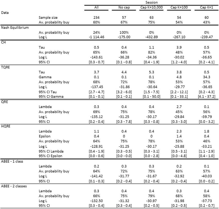
Table III reports our estimation results, and Figure 3 displays the sta-
28
Under the null hypothesis, the probability distribution of the log-likelihood ratio statis-
tic used to test nested models is approximated by a Chi-squared distribution with degrees
of freedom equal to the difference between the numbers of parameters in the two models,
while the probability distribution of the Vuong’s statistic used to test non-nested models
is a standard normal dis tribution.
22tistical tests for various models’ comparisons. The first two lines of Table
III describe our data, namely, the number of observations, and the observed
average probability to buy. The next two lines show the predictions and log-
likelihoods of the Nash equilibrium under risk neutrality.29 The mean choices
are generally far away from the Nash equilibrium; the observed probability
to buy is too low when there exists a bubble-equilibrium, and too high when
it does not exist.
Table III then provides the predictions and log-likelihoods of the vari-
ous SQRE and ABEE models including the Cognitive Hierarchy (hereafter
CH) and its extension, the Truncated Quantal Response Equilibrium (here-
after TQRE), and the Quantal Response equilibrium (hereafter QRE) and
its extensions, the Heterogeneous QRE (hereafter HQRE) and the one- and
two-classes ABEE. For brevity, the estimations of the overconfidence CH
model (hereafter OCH) and of the general SQRE model are given in the
Supplementary Appendix.
The results are as follows. The average level of sophistication τ of the
CH, estimated on the entire data set, is 0.5. This is in line with the median
estimates reported by Camerer, Ho and Chong (2004) that lie between 0.7
and 1.9, but is a little low. This low estimated τ suggests a high proportion
of level-0 players, around 60%. Interestingly, what drives this result is not
really the fact that traders enter too much into bubbles when they should not.
Indeed the fact that there is only around 10% of subjects who buy when they
know they are last in the market sequence suggests a proportion of level-0
players equal to 20%. What explains the high estimated proportion of level-0
players is rather the fact that subjects do not buy as much as expected by the
cognitive hierarchy model (with a higher average sophistication level) when
there is no cap on the initial price or when the cap is large. This can be seen
on Figure 2 that plots the predictions of the CH model using the best-fitting
value of τ estimated on the entire data set. CH embeds the better than
average effect to the extent that traders believe that no other agent does as
many steps of reasoning as them. Our estimations of OCH (reported in the
Supplementary Appendix) show that we cannot reject the hypothesis that
θ = 1, its CH restriction. Overconfidence is thus an important feature that
enables the CH logic to fit our data pretty well.
29
We consider that traders coordinate on the bubble equilibrium when there is no cap
on the initial price. The no-bubble Nash equilibrium has a lower log-likelihood. In order
to compute the likelihoods, we assume that players choose non-equilibrium strategies with
a probability of 0.0001.
23SQRE ABEE
==0 =0
p=0.804 ABEE 2 classes
TQRE p=0.008 HQRE
2
p=0.238
→∞ p=0.000 p=0.001
=0 p=0.000
1 2 2
CH p=0.011 QRE ABEE 1 class
→∞
→∞ →∞
p=0.000 p=0.000
Nash
Figure 3: Statistical tests for various models’ comparisons using parameters
estimated across all treatments. The arrows point towards the model with the
highest likelihood. Plain and dotted lines indicate, respectively, significant
and insignificant differences in likelihood.
The payoff responsiveness Λ, estimated on the entire data set, is 0.3. This
is consistent with the results of Mc Kelvey and Palfrey (1995) who report
estimates between 0.15 and 3.3. As was also the case for the CH model,
such a low value of the responsiveness parameter is required not so much to
explain why subjects buy when they should not (that is, when the offered
prices are close to the price cap, if any) but to explain why they do not buy
that much when they should (that is, when the offered prices are low).
As shown in Figure 3 that displays the statistical tests for various models’
comparisons, the QRE fits our data better than the CH model (p-value=0.01
for the overall data). This result is interesting because Camerer, Ho and
Chong (2004) show that CH fits better than QRE for a wide variety of games.
This suggests that there is a specific aspect to the nature of speculation in
the bubble game. Moreover, this result is also at odd with those of Kawagoe
and Takizawa (2010), who compare the goodness of fit of both models in
laboratory experiments of the centipede game. In order to understand why
QRE fits better than CH in the bubble game, it is interesting to focus on
the treatment with K = 1. Indeed, this treatment corresponds to a specific
centipede game with three agents playing once. In this treatment, CH ap-
pears to fit better than QRE (p-value=0.046). The other treatments with
K > 1 are not centipede games because some agents do not know what their
24position is. In this case, the information revealed by prices enable traders
to better infer their chances not to be last and affect their expected payoffs.
For these treatments, QRE fits better than CH most of the time (p-values
are 0.491, 0.064, and 0.000 for K equals 100, 10,000, and +∞, respectively).
Given that the informativeness of prices is a relevant feature from an empir-
ical point of view, this result demonstrates again the interest of our design
in better understanding the nature of speculation.
Looking at Figure 2, it seems that QRE better captures the drop in the
probability to buy for prices P ≥ 100. In the QRE, since costlier mistakes are
less likely, this model is able to capture the drop in players’ expected utility
from buying: when they are proposed a price P ≥ 100, the conditional
probability to be third is greater than or equal to 74 , whereas, when they are
proposed a price of 1 or 10, the conditional probability to be third is zero.
This informational feature is present in our design but not in the centipede
game, and has behavioral consequences in the bubble game.
We then estimate generalizations of the CH and QRE models. As Figure
3 indicates, TQRE and HQRE improve on CH and QRE models, respectively.
This suggests that taking into account heterogeneity in payoff responsiveness
enables to better fit data from the bubble game. However, HQRE still fits
better than TQRE, asserting the fact that cognitive hierarchies are not a
crucial ingredient to understand speculation in the bubble game. 30 We
thus conclude that the nature of speculation in the bubble game is related
to less than perfect payoff responsiveness as well as uncertainty concerning
this responsiveness.
We finally estimate the ABEE models that assume traders form expec-
tations within analogy classes. We find that the two-class ABEE fits the
bubble game data better than the one-class ABEE. This confirms that in-
formational aspects related to the inference on the probability not to be last
play an important role in bubble formation in our game. Moreover, the fit
of the two-class ABEE is not significantly different from the one of the QRE
and of the HQRE, suggesting that both (heterogeneous) limited payoff re-
sponsiveness and analogy-classes are important ingredients in understanding
bubble formation.
Finally, for most of the behavioral game theory models, the parameters
of interest, estimated for each treatment, display some variability: point
30
As shown in the Supplementary Appendix, the goodness of fit of HQRE is not statis-
tically different than the one of the general SQRE
25You can also read