Magnetic diffusion, inductive shielding, and the Laplace transform
←
→
Page content transcription
If your browser does not render page correctly, please read the page content below
Magnetic diffusion, inductive shielding, and the Laplace transform

                       Alexander E. Krosney,∗ Michael Lang,† Jakob J.
                       Weirathmueller,‡ and Christopher P. Bidinosti§
                       Department of Physics, University of Winnipeg,
                  515 Portage Avenue, Winnipeg, Manitoba, Canada R3B 2E9
                                     (Dated: January 23, 2021)

                                             Abstract
  In the quasistatic limit, a time-varying magnetic field inside a conductor is governed by the
diffusion equation. Despite the occurrence of this scenario in many popular physics demonstrations,
the concept of magnetic diffusion appears not to have garnered much attention itself as a subject for
teaching. We employ the model of a thin conducting tube in a time-varying axial field to introduce
magnetic diffusion and connect it to the related phenomenon of inductive shielding. We describe
a very simple apparatus utilizing a wide-band Hall-effect sensor to measure these effects with a
variety of samples. Quantitative results for diffusion time constants and shielding cutoff frequencies
are consistent with a single, sample-specific parameter given by the product of the tube radius,
thickness, and electrical conductivity. The Laplace transform arises naturally in regard to the time
and frequency domain solutions presented here, and the utility of the technique is highlighted in
several places.

                                                 1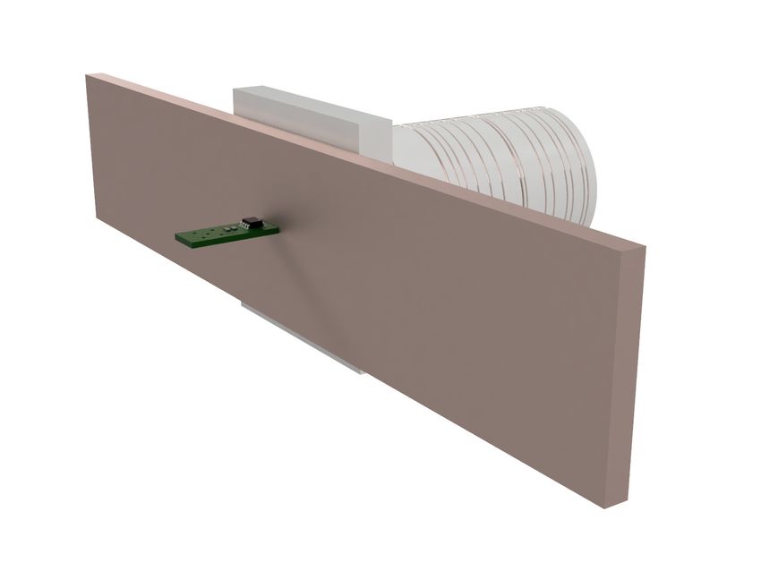
I.    INTRODUCTION

     Demonstrations of the interaction between magnetic fields and non-magnetic conducting
materials are very important – and popular. They provide strong, and often quite dra-
matic, visualizations of the Lorentz Force, Faraday’s Law, and Lenz’s Law; and are typically
employed to launch a discourse on the fact that electricity and magnetism, while seem-
ingly disparate phenomena in static configurations, are truly one and the same when time
variation occurs. Particular manifestations of such interactions, such as eddy currents or
magnetic braking, are discussed to varying degrees in standard textbooks,1–3 while much
greater variety and detail can be found in the literature.4–18
     To motivate our work on the related but seemingly lesser-known topic of magnetic dif-
fusion, we begin by writing the differential equation for a time-varying magnetic field in a
non-magnetic conductor (see for example Sec. 9.4.1 of Griffiths1 ):

                                              ∂B(r, t)        ∂ 2 B(r, t)
                          ∇2 B(r, t) = µ0 σ            + µ0              ,                 (1)
                                                ∂t                ∂t2

where µ0 is the permeability of free space and σ and  are the electrical conductivity and
permittivity of the conductor, respectively. In the limit of slowly varying fields, indicative
of the scenarios in the many papers mentioned above, the second-order time derivative
associated with the displacement current is negligible. As a result, in this quasistatic limit,
Eq. 1 is safely replaced with

                                                      ∂B(r, t)
                                  ∇2 B(r, t) = µ0 σ            ,                            (2)
                                                        ∂t

which is indeed a form of the diffusion equation,3,19–21 though it is rarely noted as such and
few of the phenomena it describes are ever regarded as diffusive processes.
     In light of this circumstance, one is tempted to re-interpret some such phenomena in terms
of magnetic diffusion. For example, an ac magnetic field impinging on a metallic enclosure
can be viewed as having insufficient time each half-cycle to fully diffuse into the conductive
structure before it must start to diffuse out again. Such an effect is exacerbated with higher
frequencies, thicker walls, and larger conductivities, all of which lead to increased inductive
shielding. This point of view also leads one to anticipate a phase lag between the applied
field and the field that has managed to diffuse into the enclosure. While this interpretation is
certainly consistent with the physics at hand, one must concede that it is not as satisfactory

                                                2
as a more intuitive, standard description in terms of induced (eddy) currents and Lenz’s
Law, say. Moreover, for the steady-state sinusoidal case, with B(r, t) = B(r)e−iwt , the
p
right hand side of Eq. 2 is readily replaced with −2iB(r)/δ 2 (where δ = 2/µ0 σω is the
electromagnetic skin depth1–3 ) which only further obscures the form and function of the
diffusion equation. It appears then that despite the generality and ubiquity of Eq. 2, the
concept of magnetic diffusion can indeed be easily overlooked.
One scenario where the notion of a magnetic field diffusing through a conductor is quite
natural and intuitive is the step response.3,19–21 Here a switched magnetic field that would
be established (near) instantaneously in the absence of the conductor now takes time to
diffuse through the bulk of the material as induced eddy currents within it decay. This
approach is well established in the research literature,22–27 but is largely unknown as a
teaching demonstration, as far as we can tell. In this paper, we present a simple experiment
that employs a wide-band Hall-effect sensor to directly monitor the process of magnetic
diffusion and determine associated time constants. The same apparatus is used without
modification to make ac measurements as a function of frequency and quantify the onset
of inductive shielding. The two phenomena are linked, of course, and we also take this
opportunity to highlight the utility of the Laplace transform for analyzing the response of
the system in both the time and frequency domains.
This paper is organized as follows. First we develop the model of the thin conducting tube
in a time-varying axial field, providing both the step and steady-state sinusoidal response
and linking the two via the Laplace transform. This model is intuitive, informative, and
easy to realize experimentally. Next we describe the apparatus and experimental procedure
that we employ at our institution as an undergraduate laboratory exercise. We then present
and discuss results for magnetic diffusion through conducting slabs and tubes, as well as
inductive shielding of the latter. In the appendices, we provide known solutions for the
general case of a conducting tube of arbitrary thickness, and also present the design method
and characterization of the coil we built to generate a highly homogeneous magnetic field
over the length of the tube samples.
3II. THE THIN CONDUCTING TUBE IN A TIME VARYING AXIAL FIELD
Following the approach of Haus and Melcher,19 we consider a long, cylindrical, non-
magnetic tube with inner radius a, outer radius b, thickness h ≡ b − a, permeability µ0 , and
conductivity σ, subject to an applied, uniform, axial magnetic field Bo (t). Assuming the
tube to be thin (b/a ≈ 1), Ampère’s law can be written as the boundary condition
Bi (t) − Bo (t) = µ0 hJ(t) , (3)
where Bi (t) is the total axial field inside the tube, J(t) is an azimuthal (eddy) current density
that is uniform over the thickness of the tube, and the quantity hJ(t) is the instantaneous
surface current that leads to the discontinuity of the field inside and outside the tube. This
is, of course, just the model of an infinitely long solenoid, which produces an axial field of
magnitude µ0 hJ(t) inside its volume and zero field outside. (Indeed, one could approach
this entire problem as a long, thin, single-turn inductor of length `, resistance R = 2πa/σh`
and inductance L = µ0 πa2 /`, as done by Íñiguez et al.9 ) The assumption that the current
density is uniform also implies that the tube is electromagnetically thin, i.e., h
δ.
From Faraday’s law of induction, we also have
dΦ
E =− , (4)
dt
where E = E(t) 2πa is the electromotive force associated with the induced electric field E(t)
driving eddy currents around the tube and Φ = Bi (t) πa2 is the magnetic flux through the
tube. Using Ohm’s law J = σE, Eq. 4 can be written as
2πa d
J(t) = −πa2 Bi (t). (5)
σ dt
Combining Eqs. 3 and 5 and rearranging leads to the differential equation
dBi (t) Bi (t) Bo (t)
+ = , (6)
dt τ τ
with time constant
τ = 12 µ0 σah , (7)
containing the sample-specific parameter (σah). Equation 6 is completely general and can
be used to determine the total magnetic field inside a thin conducting tube for any uniform
4applied field Bo (t), as is done below for a step field and a sinusoidal field. Corresponding
solutions for the general case of a tube of any thickness are presented in Appendix A.
For the step field Bo (t) = Bo for t ≥ 0, the solution for initial condition Bi (0) = 0 is
easily found to be19,20
Bi (t) = Bo (1 − e−t/τ ). (8)
The magnitude of the current density in the tube is therefore
Bo −t/τ
J(t) = e . (9)
µ0 h
Equations 8 and 9 show that the application of a dc step field leads, by Lenz’s Law, to an
induced field that opposes Bo . The overall interpretation is that the applied field diffuses
into the tube with the same characteristic time as the decay of the induced current. Since
τ depends not only on the tube dimensions but also its composition, materials with high
conductivity, such as copper, will produce long-lasting induced currents (i.e., slow diffusion
of Bo ), whereas a poor conductor will produce short-lived induced currents (i.e., fast diffusion
of Bo .)
We now consider an ac field of the form Bo (t) = Bo e−iωt , with frequency independent
magnitude Bo . For the steady-state sinusoidal response, one anticipates a solution of the
form Bi (t) = Bi (ω)e−iωt . By substituting Bo (t) and Bi (t) into Eq. 6, one finds the complex
amplitude8,9,17,22
Bo
Bi (ω) = , (10)
1 − iωτ
which reduces to Bi (ω) ≈ Bo (1+iωτ ) at low frequency9,10 and goes to zero at high frequency.
From this result, the induced magnetic field generated by J(t) is easily determined:
iωτ
Bi (t) − Bo (t) = Bo (t) . (11)
1 − iωτ
As expected, it is 90◦ out of phase with the applied field and tends to zero as ω → 0 (i.e.,
ωL
R, poor shielding), while it is 180◦ out of phase with the applied field and approaches
−Bo (t) as ω → ∞ (i.e., ωL
R, complete shielding).
The relative magnitude of the net internal field can be written as
|Bi (ω)| 1
=p (12)
Bo 1 + (ωτ )2
1
=p , (13)
1 + (ah/δ 2 )2
5and the onset of inductive shielding is seen to occur at a cutoff frequency
fc ≡ (2πτ )−1 (14)
= (πµ0 σah)−1 , (15)
which can also be cast as a critical thickness
hc ≡ δ 2 /a (16)
= (πµ0 σaf )−1 . (17)
The latter result, noted by Fahy et al.,8 often comes as a surprise: It says that the onset of
shielding for this geometry occurs not when the skin depth is comparable to the thickness
of the tube (δ ∼ h) – a commonly held misconception – but when δ 2 ∼ ah.8,28 As a result,
an electromagnetically thin tube with h
δ can still provide efficient shielding if a
δ.
We end here by re-deriving the above results via the Laplace transform approach. In
doing so, our intention is not to provide an overview of such methods – which are well
described in many standard textbooks29–32 and are further discussed in the pedagogical
literature33,34 – but rather to take the opportunity to highlight this elegant mathematical
tool in the context of a very interesting and simple electromagnetic system. We will also
use the Laplace transform in two other instances in this paper, making use of standard
transform-pair lookup tables throughout.29–32
The Laplace transform of Eq. 6 with initial condition Bi (0) = 0 is
Bi (s) Bo (s)
sBi (s) + = , (18)
τ τ
where B(s) denotes the transform of a magnetic field B(t) and s is a complex frequency in
general. Solving for Bi (s) gives the Laplace transform of Bi (t):
Bo (s)
Bi (s) = . (19)
1 + sτ
For the dc step field turned on at t = 0, Bo (s) = Bo /s and Eq. 19 becomes
Bo
Bi (s) = , (20)
s + s2 τ
which has inverse transform Bi (t) = Bo (1 − e−t/τ ), identical to Eq. 8.
The steady-state sinusoidal response, on the other hand, is given by Bi (t) = H(s) Bo e−iωt
with transfer function H(s) ≡ Bi (s)/Bo (s) found from Eq. 19 and evaluated at s = −iω.31
6This gives
Bo
Bi (t) = e−iωt , (21)
1 − iωτ
where the term in braces is the complex amplitude of Eq. 10. It is also worth noting that
the transfer function found here is identical to that of a low-pass filter, which is expected
intuitively for inductive shielding (i.e., low frequencies pass through the tube, high frequen-
cies do not) and also given that an equivalent LR circuit model can be used to analyze this
system.9
III. EXPERIMENTAL METHOD
We now describe the apparatus and experimental procedure that we use an undergraduate
laboratory exercise to make quantitative studies of magnetic diffusion and inductive shielding
in conducting tubes based on the preceding theoretical model. We also present an ancillary
experiment using conducting slabs that provides a very simple and intuitive demonstration
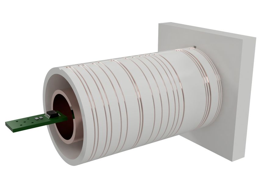
of magnetic diffusion. The two experimental configurations are shown in Fig. 1.
The specific details of the various measurements, as well as the dimensions and properties
of the different samples, are presented further below. In general, however, the experimental
procedure is quite simple. An electromagnetic coil, described in detail in Appendix B, is
driven by a waveform generator (Rigol DG1032Z) to generate the applied magnetic field.
Field measurements are made by a Hall-effect sensor (Sentron CSA-1VG)35 with its differen-
tial output connected to two separate channels of an oscilloscope (Agilent DSO-X 2014A).
The internal math function of the oscilloscope is used to determine the difference of the
two channels, providing a final signal that is proportional to the magnetic field at the lo-
cation of the sensor. Signal averaging using the built-in functionality of the oscilloscope is
also employed. The addition of a differential amplifier between the sensor and oscilloscope
could further improve performance,28,36 but was purposely omitted here in order to keep
the apparatus as simple as possible and hopefully further encourage the adoption of mag-
netic diffusion and ac shielding studies in the undergraduate teaching lab. The 100-kHz
bandwidth of the sensor35,36 is suitable for the time and frequency scales explored here.
7Conductive Slab
Hall Effect Sensor
Electromagnetic Coil
Conductive Tube
FIG. 1. Cutaway models of the two experimental configurations. The 3D-printed coil former
(white) was made as a single piece with grooves for wire windings and square end supports that
act as a stand. Top: the conductive slab is placed between the Hall-effect sensor and one end of
the coil. Bottom: the sensor is placed at the center of the coil and conductive tube. Both the
sensor and tube are held in position by additional 3D-printed parts, which are not shown.
A. Step field measurements
Step field measurements were performed by driving the coil with a 50-Hz square-wave
voltage alternating between zero and 7.5 V. The input couplings of the oscilloscope were
set to dc and 256 averages were used. Because the analog output channel of the Hall-
effect sensor is referenced to its common output channel held at 2.5 V (giving a full scale
differential output of ±2.5 V),35 the gain of both scope channels was set to 500 mV/div. An
offset of 2.5 V was applied to both channels and the sensitivity of the math waveform was
set to 10 mV to capture the much smaller differential signal. The time constant of our coil
is calculated to be 2.2 µs (L = 129 µH, R = 8.13 Ω + 50 Ω from the Rigol DG1032Z output),
8which is less than both the scan time (∼ 3 µs) and rise time (∼ 3 µs) of the sensor35,36 and
does not limit the overall bandwidth of the system. The signal of a step field measurement
performed at the center of the coil in the absence of any conducting sample is shown in
Fig. 2.
20
15
10
Signal (mV)
5
0
5
10
-6 -3 0 3 6 9 12 15 18 21
Time ( s)
FIG. 2. The differential signal from the oscilloscope for a step field measurement using the con-
figuration shown in the bottom of Fig. 1 with no tube. The red line is an exponential fit to the
data assuming an offset of exactly 3 µs to account for the sensor scan time. The fit yields a time
constant of 2.1 µs, consistent with the quoted rise time of the sensor and previous tests.35,36
Given the finite bandwidth of the Hall-effect sensor, its output signal S(t) must also be
determined by the differential equation for a low-pass filter:
dS(t) S(t) kB(t)
+ = , (22)
dt τf τf
where B(t) is the magnetic field at the location of the sensor, τf is the time constant (or
rise time) of the sensor, and k is its sensitivity (∼ 280 V/T for the CSA-1VG).35 For a
magnetic field of the form of Eq. 8, one can solve Eq. 22 directly by standard methods for
linear first-order equations.29,30 Conversely, one can solve by Laplace transform. By analogy
with Eqs. 6 and 18, then, and by making use of Eq. 20 for the Laplace transform of the field
of Eq. 8, one quickly finds the Laplace transform of S(t):
1 So
S(s) = , (23)
1 + sτf s + s2 τ
9where So = kBo . The general solution for the sensor output, along with two particularly
useful limits, is thus
τf e−t/τf − τ e−t/τ
S(t) = So 1 − (24)
τf − τ
t + τ −t/τ
= So 1 − e when τf = τ , (25)
τ
→ So 1 − e−t/τ
when τf
τ . (26)
One can also derive Eq. 24 from the Laplace convolution of So (1 − e−t/τ ) with the impulse
response of the low pass filter (1/τf )e−t/τf .29–32
Given that the magnetic diffusion time constants measured in this work are around two
orders of magnitude larger than the rise time of the Hall-effect sensor (τf ∼ 3 µs), Eq. 26 is
appropriate here. As a result, we use as a fit function
S(t) = So 1 − e−(t−ts )/τ ,
(27)
where ts = 3 µs is the scan time of the sensor and time t is measured with respect to the
function generator trigger corresponding to the rising edge of the square-wave drive voltage.
If thinner tubes (i.e., shorter τ ) or narrower-band sensors (i.e., longer τf ) are employed, one
may need to use Eq. 24 instead. Lastly, we note that given the very similar time constants
of our coil and sensor, the exponential fit in Fig. 2 could be replaced by something akin to
Eq. 25. This has little bearing on our present study, however, and a more detailed analysis
is unwarranted here.
B. ac field measurements
Here the coil is driven by a 15 Vpp sine wave at 101 logarithmically-spaced frequencies over
the range f = 1 to 10,000 Hz. The oscilloscope couplings and sensitivities are the same as the
previous section. Over this frequency range, the magnitude of the drive circuit impedance
increases by only 1%; however, the phase varies by about 8◦ , which is not insignificant.
To account for these changes, as well as any potential frequency dependence in the receive
chain, we also recorded the phase of the differential signal (relative to the trigger) and
repeat the same set of frequency measurements with and without the conducting tubes.
The latter represents a background measurement that is used to correct the tube data with
respect to the phase and magnitude of the applied field at each frequency. A similar process
10has been described elsewhere.13 Custom Python code was written to automatically pass
frequencies to the waveform generator and return amplitude and phase measurements from
the oscilloscope. Signal averaging is set to 16 for the lowest frequencies and is dynamically
increased via the program for higher-frequency measurements with tubes, which otherwise
would suffer from reduced signal-to-noise ratio (SNR) due to greater inductive shielding.
Overall, this strategy helps minimize run time. From Eqs. 13 and 14, data for the corrected
signal amplitude are fit to the following function to extract the cutoff frequency fc :
So
|S(f )| = p (28)
1 + (f /fc )2
C. Samples
The response to a step field applied perpendicular to the face of a slab was measured
for three samples – one each of copper, brass, and plastic. The nominal dimensions of the
slabs – which were in fact borrowed from our own sliding magnet demo – are 10 inches long,
2 inches wide, and 1/4 inch thick. The response to both step and ac fields applied along
the axis of a tube was measured for three samples – two of copper and one of aluminum
– each nominally 6 inches long, but with different diameters and thicknesses. The precise
dimensions and measured conductivities of the tubes, which are needed for a quantitative
analysis of magnetic diffusion and inductive shielding via the models in Section II, are given
in Table I. The length `, outer diameter 2b and thickness h of the tubes were measured with
digital calipers at five different positions each to account for non-uniformities. The resistivity
ρ of the samples was determined via a standard 4-wire measurement by driving a known
current I through the tubes and measuring the voltage drop V across them with a digital
multimeter (Agilent 34411A). From V = IR and R = ρ`/A, where A is the cross-sectional
area of the tube and a = b − h is its inner radius, one finds
1 V π(b2 − a2 ) V π(2bh − h2 )
≡ρ= = . (29)
σ I ` I `
11Tube h (mm) b (mm) ` (mm) V (µV) ρ (10−8 Ω·m) σ (107 S/m)
Copper #1 0.804(7) 6.357(9) 153.0(5) 422(2) 1.66(3) 6.02(11)
Aluminum 1.468(5) 12.706(4) 153.5(5) 313(3) 4.50(5) 2.22(2)
Copper #2 1.672(15) 9.507(6) 152.0(5) 144.4(7) 1.73(2) 5.78(6)
TABLE I. Measured properties of the tube samples. The numbers in parentheses are the uncer-
tainty in the last digit(s) of each quantity, as determined by standard techniques.37 The tubes are
seamless and we assume their electrical properties to be isotropic. A dc current of 5.000(5) A was
used for all resistivity measurements.
IV. RESULTS AND DISCUSSION
A. Magnetic diffusion through slabs and tubes
The results for the slabs are shown in Fig. 3. The SNR is poor for these measurements
largely due to the much weaker applied field at the location of the sensor in this configuration
(see Figs. 1 and 8.) This could be improved by using a small, flat coil of many turns placed
directly on the face of the slab. Still, the results presented here clearly demonstrate that,
as expected, magnetic diffusion through copper is slower than it is through brass, since
the former is the better conductor. Also, the step field is seen to pass through the non-
conducting plastic slab near-instantaneously (i.e., indistinguishable from the rise time in
Fig. 2.) Another result worth noting in Fig. 3 is the near-instantaneous jump seen in the
field for copper and brass when the sensor is placed directly behind the slab but not on the
center line (or axis) of the coil. By symmetry, it is only at the central location where the net
field is expected to be uniquely zero just after the coil is turned on. At any other location,
the induced field does not necessarily cancel the applied field. Equivalently, one can think of
this result as being a consequence of the magnetic field lines initially wrapping around the
exterior of the slab while its interior is still fully shielded by the induced currents. Again,
because of symmetry, there can be no magnetic field at the central point located directly
on the back (or front) face of the slab, since the approaching field lines must spread out in
opposite directions about this point.
121.0
1.0
a b
0.8 c
0.6
0.8
0.4
0.2
Normalized Magnetic Field
0.6 (a) Plastic
0.0 (b) Brass
(c) Copper
1.0 a
0.4 b
0.8
c
0.6
0.4
0.2
0.2
0.0
0.0
0.0 0 0.2 2 0.4 4 0.6 6 0.8 8 1.0
Time (ms)
FIG. 3. The magnetic field measured at the face of the slabs opposite to the coil. The legend
refers to both graphs. Top: results for a measurement position that is on the center line of the
coil. Bottom: results for a measurement position that is 2.5 mm away from the center line toward
the top of the slab.
The results for the tubes are shown in Fig. 4 along with a background measurement (i.e.,
no tube) for comparison. Time constants are determined from fits to Eq. 27 with ts = 3 µs
and are compiled in Table II along with predicted values from the thin-tube model. Our
results largely agree with the rule-of-thumb that the thin-tube model should be good to
within ∼ 10% for a/b ≥ 2/3.20,25 The greatest discrepancy is seen with our thickest sample,
which perhaps suggests that one should use tubes with a/b closer to 0.9, say, if the goal is
13to provide teaching demonstrations that agree very closely with the thin-tube model. We
also point out that time constants predicted from the general model (Eq. A6) are closer to,
but still do not agree within error, with our measured values. Still, these results provide
an excellent demonstration of magnetic diffusion, consistent with the trends predicted from
measured sample properties. With a good degree of confidence, then, we use our values of
τfit here to predict the cutoff frequencies for the ac measurements of the next section. These
are also listed in Table II.
1.0
0.8
Normalized Magnetic Field
0.6
0.4
0.2 Background
Copper #1
Aluminum
0.0 Copper #2
0.5 0.0 0.5 1.0 1.5 2.0 2.5 3.0
Time (ms)
FIG. 4. The magnetic field measured at the center of the tubes. For clarity only every 50th data
point is shown. The solid lines are least-square fits to Eq. 27 for all data at t ≥ ts = 3 µs.
Tube a/b τthin (µs) τfit (µs) fc (Hz)
Copper #1 0.874(2) 169(4) 179.3(2) 887.8(7)
Aluminum 0.8845(6) 230(3) 244.9(2) 649.9(5)
Copper #2 0.824(2) 476(7) 544.5(6) 292.3(3)
TABLE II. Ratios of tube radii; the time constants predicted from the thin-tube model using the
values given in Table I; the measured time constants extracted from fits to the data in Fig. 4; and
the cutoff frequencies calculated from τfit via Eq. 14.
14B. Inductive shielding by tubes
Example data of the ac signals measured at the center of the tubes are shown in Fig. 5
for a drive frequency of 1 kHz. At this frequency, all samples exhibit a clear phase shift
with respect to the voltage trigger, as well as a reduction in amplitude with respect to the
background value. These are both hallmarks of the presence of eddy currents and thus the
onset of inductive shielding. (Indeed, it is very informative for students to simply observe
how the signal on the oscilloscope changes for a given sample as they increase the drive
frequency on the function generator.) From the comparative results shown in Fig. 5, it is
also clear that the degree of shielding for the different tubes is consistent with their respective
cutoff frequencies predicted from the diffusion measurements above (Table II) or by what
one would estimate from their properties in Table I via Eq. 15.
(a) Voltage Trigger (c) Copper #1 (e) Copper #2
(b) Background (d) Aluminum
1.0 a
b
c
0.5
d
Normalized Signal
e
0.0
0.5
1.0
0.00 0.25 0.50 0.75 1.00 1.25 1.50
Time (ms)
FIG. 5. Signal waveforms at a drive frequency of 1 kHz. Amplitudes are normalized with respect
to the background value (21.9 mV) measured here.
It is also possible to discern a small phase shift in the background signal in Fig. 5. This
is due to the complex impedance of the drive circuit arising from the inductance of the coil.
To correctly extract the complex components of the field inside the tubes, the raw data of
the type shown in Fig. 5 must be corrected with respect to the phase and amplitude of the
background signal at each frequency as discussed in Section III B. The results of this process
15are shown in Fig. 6 for the two copper samples. Overlaid on top of these data are curves
for the general model (Appendix A), the thin-tube model, and the low-frequency limit of
the latter generated using the sample properties given in Table I. The low-frequency model
proposed by Íñiguez et al.9,10 is suitable to a few hundred hertz or less for these samples, while
the thin-tube model can extend the range of study by perhaps another order of magnitude.
The general model, on the other hand, provides excellent agreement over the full frequency
range studied here. The limitation of the thin-tube model is easily understood from the
well-known rule-of-thumb that the skin depth of copper is roughly 1 cm at 60 Hz, which
translates to 3 mm at 670 Hz or 1 mm at 6 kHz. Looking at the copper tube thicknesses
given in Table I, then, one sees that the condition of being electromagnetically thin (i.e.,
h
δ) will certainly break down over the frequency range studied here, and deviations from
the thin-tube model are to be expected at the higher frequencies.
161.0
1.0
0.8 Copper #1
0.8
0.6
Real
Imaginary
0.4
0.2
Normalized Magnetic Field
0.6
0.0
1.0
0.4
0.8 Copper #2
0.6
0.4
0.2
0.2
0.0
0.0
0.0100 0.2 101 0.4 102 0.6 103 0.8 1041.0
Frequency (Hz)
FIG. 6. Complex components of the internal magnetic field for the copper tubes. The legend
refers to both graphs. The solid and dash-dotted lines are the functional form for the general
model (Eq. A7) and the thin-tube model (Eqs. 13 and 7), respectively. The dashed lines are the
low-frequency limit9,10 of the latter as discussed in Section II.
17To better highlight the inductive shielding of the tubes, as well as their behavior as low-
pass filters, the magnitude of the internal field is plotted versus frequency in Fig. 7 for all
tube samples. The low-frequency end of the data are fit to Eq. 28 and cutoff frequencies are
compiled in Table III along with predicted values from the thin-tube model. We chose to
limit the fitting range to data with normalized amplitude greater than 0.5, which from Fig. 6
still show good agreement with the thin-tube model. The predicted cutoff frequencies from
Table II are also presented in Fig. 7 and show good agreement with the ac measurements. A
final feature of interest in Fig. 7 is the slight decrease in amplitude seen in the background
measurement at high frequencies. This again is due to the small increase in coil impedance;
all sample data have been corrected for this by normalizing to the background amplitude at
each frequency value as mentioned above. With regard to the results in Table III, one can
see that all measured values of cutoff frequency agree to within a few percent or less with
the values predicted from the thin-tube model. Also, as shown in the last two columns of
the table, the onset of inductive shielding does indeed occur when δ 2 ∼ ah and not when
δ ∼ h.8,28
Tube fc,thin (Hz) fc,fit (Hz) h/δ ah/δ 2
Copper #1 942(20) 946(2) 0.381(8) 1.00(4)
Aluminum 691(8) 710(1) 0.366(4) 1.03(2)
Copper #2 335(5) 327(1) 0.457(7) 0.98(2)
TABLE III. Cutoff frequencies predicted for the thin-tube model using the values given in Table I;
the measured cutoff frequencies extracted from fits to the data in Fig. 7; and the ratios h/δ and
ah/δ 2 calculated from fc,fit .
181.0
0.8
Normalized Magnetic Field
0.6
0.4
0.2 Background
Copper #1
Aluminum
Copper #2
0.0
100 101 102 103 104
Frequency (Hz)
FIG. 7. Normalized magnitude of the internal field as a function of frequency. The solid lines are
least-square fits of Eq. 28 to all data points with ordinate value greater than 0.5. The horizontal
√
dashed line indicates the half-power amplitude 1/ 2 that defines the cutoff frequency of a low-
pass filter. The vertical dashed lines indicate the cutoff frequency predicted for each tube from the
preceding step field measurements (see Table II).
V. CONCLUSION
A review of the literature reveals that the concept of magnetic diffusion is rarely con-
sidered for the purposes of pedagogy. The thin conducting tube in a uniform, time-varying
axial field provides a complete and very accessible model for exploring magnetic diffusion
as well as the related phenomenon of inductive shielding. The product of the tube radius,
thickness, and electrical conductivity provides a single, sample-specific parameter that sets
both the time constant for stepped dc fields to diffuse through the tube and the cutoff fre-
quency for ac fields to penetrate the interior of the tube. While not required, the use of
the Laplace transform to solve for and link the time and frequency domain solutions of this
system further broadens the educational experience here.
A simple apparatus utilizing a wide-band Hall-effect sensor allows either stepped or ac
measurements without any configurational changes. The addition of a differential amplifier
following the Hall-effect sensor could further improve performance. As it stands, the present
19setup provides more than sufficient SNR to make meaningful qualitative and quantitative tests on a variety of samples. Time constants and cutoff frequencies extracted from the two types of measurement for conducting tubes show good agreement with each other as well as with predicted values. Through a judicious choice of frequency range and tube thickness, one can design a student laboratory experiment that resides fully within the limits of the thin-tube model (h
and Jν and Yν are Bessel functions of the first and second kind of order ν. After sufficient
time has passed (t > µ0 σ/γ12 ), the field within the conductor volume can described by the
n = 1 term only. In this case the field is once again given by Eq. 8 with time constant20
                                                    µ0 σ
                                              τ=         .                                 (A6)
                                                    γ12
   For an ac field Bo (t) = Bo e−iωt , the solution for the complex amplitude of the internal
field is8,22
                                      2
                        Bi (ω) = Bo       [I0 (zo )K2 (zi ) − K0 (zo )I2 (zi )]−1 ,        (A7)
                                      zi2
where zi = (1 − i)a/δ, zo = (1 − i)b/δ, and Iν and Kν are modified Bessel functions of the
first and second kind of order ν. One can show that this is equivalent to the result given by
Íñiguez et al.,11 keeping in mind that the latter employs eiωt for the temporal dependence
of the applied field which leads to a conjugate solution.
   Finally, based on the discussion in Section II, the Laplace transform of Bi (t) for the step
response divided by the Laplace transform of the step function (1/s) should lead to the
complex amplitude Bi (ω) for the steady-state sinusoidal response. The procedure is trivial
here and starting from Eq. A2 one quickly arrives at
                                                     ∞
                                                                      !
                                                    X     cn τn
                              Bi (s) = Bo       1−s                       ,                (A8)
                                                    n=1
                                                        1 + τn s

which evaluated at s = −iω gives an alternative form of Eq. A7. We have shown the
two solutions to be numerically equivalent for the tube parameters and frequency range
studied here. We did not attempt to prove mathematical equivalence, although it appears
the necessary details can be gleaned from the work of Jaeger.23
   The solutions presented in this appendix are also valid for a non-magnetic, conducting
tube in a uniform, transverse ac magnetic field.22,23 As a result, they also hold for a uniform
ac field applied at any angle to the axis of the tube. This is not the case for the more general
scenario of a magnetic tube, however.21–23

   Appendix B: Numerical optimization of the drive coil for improved homogeneity

   We originally built a standard solenoid comprising two layers of 100 evenly-spaced wind-
ings to serve as a drive coil. The solenoid was wound with #32 AWG enamelled magnet
wire on a 3D-printed former. We found the time constant of this coil was greater than that

                                                 21
of the Hall-effect sensor (see Fig. 2) and we decided to re-make it with the same dimensions
and wire but using only 50 windings per layer. We also took this opportunity to optimize
the winding pattern to provide greater field homogeneity over the length of the tube sam-
ples. While this does offer greater fidelity with our theoretical models, it is not critical for
obtaining satisfactory results, and preliminary tests with our original solenoid did yield near
identical time constants and cutoff frequencies to those reported above.
The details of the optimization algorithm are given below. The final winding pattern
and 3D former can be seen in Fig. 1. The specific locations of the current loops are given
in Table IV, allowing one to easily duplicate our coil or scale it to any desired radius.
The calculated magnetic field profiles of the optimized coil and the original solenoid are
shown in Fig. 8, along with those of the well-known Lee-Whiting and Helmholtz designs38
for comparison. The parameters of the various coils are summarized in Table V. For the
Lee-Whiting and Helmholtz coils, we considered two designs: fixing either their length
or their radius to equal those of our solenoid and optimized coil. Measurements of the
field profile along the axis of the optimized coil are also shown in Fig. 8 and confirm the
expected improvement in homogeneity. Accurate measurements of the off-axis field are more
challenging to achieve and were not pursued here. However, for an axisymmetric coil such
as this, the constraint of Maxwell’s equations ensures that the homogeneity of the field away
from the central axis must similarly improve.39
±zi /R
0.163 0.887 1.744 2.350 3.129
0.234 1.195 1.933 2.997 3.140
0.426 1.250 2.098 3.052 3.396
0.525 1.261 2.201 3.063 3.451
0.745 1.555 2.339 3.118 3.505
TABLE IV. The axial positions of the current loops comprising the optimized coil in ascending
order by column. The values, normalized to the coil radius R and rounded to the third decimal
point, give the distance zi to the i-th loop on either side of the central plane of the coil (z = 0). For
our coil R = 2.28 cm, which is the average radius for the two layers of #32 AWG wire (thickness
0.2 mm).
22Coil χ (µT/A/turn) N R (cm) L (cm)
Opt 6.55 100 2.28 7.98
Sol 7.51 200 2.28 7.98
LW-1 4.07 26 8.48 7.98
H-1 2.82 2 15.95 7.98
LW-2 15.18 26 2.28 2.14
H-2 19.76 2 2.28 1.14
TABLE V. Coil parameters for the optimized (Opt), solenoid (Sol), Lee-Whiting (LW) and
Helmholtz (H) coils. The coil efficiency χ is defined here as the calculated central field strength
Bz (0, 0) per unit current divided by the total number of turns N comprising each coil type. The
coil radius R is taken to be the average of the two layers for the Opt and Sol designs; while all
turns are assumed to exist on the same radius for the LW and H designs. The half-length L is the
axial location of the outermost current loop for all designs.
231.0
1.01
1.00
0.99
1.00
0.8
0.90
0.80
0.70
0.6
Normalized Magnetic Field
0.60 Opt
Sol
LW-1
0.50 H-1
1.00
0.4
0.80
0.60
0.2
0.40
0.20 Opt
Sol
LW-2
0.00 H-2
0.0
-8
0.0 -6 0.2 -4 -20.4 0 0.62 4 0.8 6 81.0
z-position (cm)
FIG. 8. Calculated profiles of Bz (0, z) for the various coils listed in Table V. The vertical dashed
lines indicate the optimization region of z = ±7.5 cm. Measurements of the optimized coil made
with the Hall-effect sensor (circles, top panel) confirm a field homogeneity within 1% over almost
the full length of the tubes used here. The Lee-Whiting and Helmholtz coils would require a large
radius (middle panel) to achieve a comparable homogeneity.
Our design optimization was performed by considering the net axial field produced by
24the sum of contributions from the symmetric pairs of current loops1–3 comprising the coil:
N/2
X µ0 R2 I/2 µ0 R2 I/2
B(z) = + , (B1)
i
(R2 + (z − zi )2 )3/2 (R2 + (z + zi )2 )3/2
where zi is the distance to the i-th loop on either side of the central plane of the coil and the
current I was set to unity. To begin, all loops are evenly spaced as per a regular solenoid.
Optimizing the axial field homogeneity over a distance zopt requires minimizing the integral
Z zopt
B(z) − B(0)
dz. (B2)
0 B(0)
This was done by randomly selecting a pair of symmetric loops and displacing them a
distance δz away from and towards z = 0. If either displacement reduces Eq. B2, the changes
are saved and another pair is randomly selected; otherwise, the changes are discarded.
Random selection continues until further displacement of all pairs does not result in an
improvement, in which case the value of δz is decreased. Once δz is reduced beyond a set
minimum threshold value (typically given by the resolution of the 3D printer) the program
exits and saves the final zi values.
To prevent overlap and wire grooves with a separation wall smaller than printing capa-
bilities, additional constraints are placed on the current loop locations. If moving a pair
places their wires within a minimum threshold distance relative to another pair, two calcu-
lations are performed. The first bundles the neighboring wires such that they form adjacent
windings within a single groove. Alternatively, the wires are spaced exactly by the mini-
mum threshold value. If either scenario improves field homogeneity, the changes are saved;
otherwise, they are discarded.
ACKNOWLEDGMENTS
We gratefully acknowledge the support of the Natural Sciences and Engineering Research
Council of Canada, especially the Undergraduate Student Research Awards for AEK and
JJW.
∗ Electronic mail: krosney-a83@webmail.uwinnipeg.ca
† Electronic mail: mlang.physics@gmail.com
25‡ Electronic mail: weirathj@myumanitoba.ca; Present address: Max Rady College of Medicine,
University of Manitoba, 750 Bannatyne Avenue, Winnipeg, Manitoba, Canada R3E 0W2
§ Author to whom correspondence should be addressed; electronic mail: c.bidinosti@uwinnipeg.ca
1 D.J. Griffiths, Introduction to Electrodynamics, 4th Ed. (Pearson, Boston, 2013).
2 G.L. Pollock and D.R. Stump, Electromagnetism (Addison Wesley, San Francisco, 2002).
3 A. Garg, Classical Electromagnetism in a Nutshell (Princeton University Press, Princeton,
2012).
4 W.M. Saslow, “Maxwell’s theory of eddy currents in thin conducting sheets, and applications
to electromagnetic shielding and MAGLEV,” American Journal of Physics 60, 693–711 (1992).
5 M.A. Nurge et al., “Drag and lift forces between a rotating conductive sphere and a cylindrical
magnet,” American Journal of Physics 86, 443–452 (2018).
6 M.H. Partovi and E.J. Morris, “Electrodynamics of a magnet moving through a conducting
pipe,” Canadian Journal of Physics 84, 253–271 (2006).
7 B. Irvine et al., “Magnet traveling through a conducting pipe: A variation on the analytical
approach,” American Journal of Physics 82, 273–279 (2014).
8 S. Fahy et al., “Electromagnetic screening by metals,” American Journal of Physics 56, 989–992
(1988).
9 J. Íñiguez et al., “Measurement of the electrical conductivity of metallic tubes by studying
magnetic screening at low frequency,” American Journal of Physics 73, 206–210 (2005).
10 J. Íñiguezet al., “Measurement of electrical conductivity in nonferromagnetic tubes and rods at
low frequencies,” American Journal of Physics 77, 949–953 (2009).
11 J. Íñiguez et al., “The electromagnetic field in conductive slabs and cylinders submitted to a
harmonic longitudinal magnetic field,” American Journal of Physics 77, 1074–1081 (2009).
12 C.P. Bidinosti et al., “The sphere in a uniform rf field – revisited,” Concepts in Magnetic
Resonance 31B, 191–202 (2007).
13 M.L. Honke and C.P. Bidinosti, “The metallic sphere in a uniform ac magnetic field: A simple
and precise experiment for exploring eddy currents and non-destructive testing,” American
Journal of Physics 86, 430–438 (2018).
14 J.R. Nagel, “Induced eddy currents in simple conductive geometries: mathematical formalism
describes the excitation of electrical eddy currents in a time-varying magnetic field,” IEEE An-
tennas and Propagation Magazine 60, no.1, 81-88 (2018). See also “Correction,” IEEE Antennas
26and Propagation Magazine, 60, no. 4, 83 ( 2018).
15 P.J.H. Tjossem and E.C. Brost, “Optimizing Thomson’s jumping ring,” American Journal of
Physics 79, 353–358 (2011).
16 C.L. Ladera and G. Donoso, “Unveiling the physics of the Thomson jumping ring,” American
Journal of Physics 83, 341–348 (2015).
17 R.W. Latham and K.S.H. Lee, “Theory of inductive shielding,” Canadian Journal of Physics
46, 1745–1752 (1968).
18 J.R. Reitz, “Forces on moving magnets due to eddy currents,” Journal of Applied Physics 41,
2067–2071 (1970).
19 H.A. Haus and J.R. Melcher, Electromagnetic Fields and Energy (Prentice-Hall, Englewood
Cliffs, 1989), Chapter 10.
20 H.E. Knoepfel, Magnetic Fields: A Comprehensive Theoretical Treatise for Practical Use (John
Wiley & Sons, New York, 2000), Chapter 4.
21 W.R. Smythe, Static and Dynamic Electricity, 2nd Ed. (McGraw-Hill, New York, 1950), Chap-
ter XI.
22 L.V. King, “XXI. Electromagnetic shielding at radio frequencies,” The London, Edinburgh, and
Dublin Philosophical Magazine and Journal of Science, 15:97, 201–223 (1933).
23 J.C. Jaeger, “III. Magnetic screening by hollow circular cylinders,” The London, Edinburgh,
and Dublin Philosophical Magazine and Journal of Science, 29:192, 18–31 (1940).
24 C.P. Bean et al., “Eddy-current method for measuring the resistivity of metals,” Journal of
Applied Physics 30, 1976–1980 (1959).
25 M.A. Weinstein, “Magnetic decay in a hollow circular cylinder,” Journal of Applied Physics 33,
762 (1962).
26 K. Lee and G. Bedrosian, “Diffusive electromagnetic penetration into metallic-enclosures,” IEEE
Transactions on Antennas and Propagation 27, 194–198 (1979).
27 M.J. Ramos et al., “The phase angle method for electrical resistivity applied to the hollow
circular cylinder geometry,” Journal of Applied Physics 67, 1167–1169 (1990).
28 C.P. Bidinosti and M.E. Hayden, “Selective passive shielding and the Faraday bracelet,” Applied
Physics Letters 93, 174102 (2008).
29 M.L. Boas, Mathematical Methods in the Physical Sciences, 3rd Ed. (John Wiley & Sons, Hobo-
ken, 2006), Chapter 8.
2730 K.F. Riley, M.P. Hobson, and S.J. Bence, Mathematical Methods for Physics and Engineering,
3rd Ed. (Cambridge University Press, Cambridge, 2006), Chapter 13.
31 C.A. Desoer and E.S. Kuh, Basic Circuit Theory (Mcgraw-Hill, New York, 1969), Chapter 13.
32 I.S. Gradshteyn and I.M. Ryzhik, Table of integrals, series, and products, 7th Ed. (Elsevier,
Amsterdam, 2007), Chapter 17.
33 K. Riess, “Some applications of the Laplace Transform,” American Journal of Physics 15, 45–48
(1947).
34 C.L. Bohn and R.W. Flynn, “Real variable inversion of Laplace transforms: An application in
plasma physics,” American Journal of Physics 46, 1250–1254 (1978).
35 See datasheet and application notes – in particular Current Sensing with the CSA-1V – at
the distributor website: https://gmw.com/product/csa-1vg-so/. The CSA-1V comes a in a
standard, surface mount SOIC-8 package, for which small breakout PCBs can be purchased
from many vendors.
36 C.P. Bidinosti et al., “A simple wide-band gradiometer for operation in very low background
field,” Concepts in Magnetic Resonance 37B, 1–6 (2010).
37 J.R. Taylor, An Introduction to Error Analysis: The Study of Uncertainties in Physical Mea-
surements, 2nd Ed. (University Science Books, Sausalito, 1996), Chapter 3–4.
38 J.L. Kirschvink, “Uniform magnetic fields and double-wrapped coil systems: Improved tech-
niques for the design of bioelectromagnetic experiments,” Bioelectromagnetics 13, 401–411
(1992).
39 S.R. Muniz and V.S. Bagnato, “Analysis of off-axis solenoid fields using the magnetic scalar
potential: An application to a Zeeman-slower for cold atoms,” American Journal of Physics 83,
513–517 (2015).
28You can also read